Bayesian Protein Sequence and Structure Alignment

Abstract

The structure of a protein is crucial in determining its functionality, and is much more conserved than sequence during evolution. A key task in structural biology is to compare protein structures in order to determine evolutionary relationships, estimate the function of newly-discovered structures, and predict unknown structures. We propose a Bayesian method for protein structure alignment, with the prior on alignments based on functions which penalise “gaps” in the aligned sequences. We show how a broad class of penalty functions fits into this framework, and how the resulting posterior distribution can be efficiently sampled. A commonly-used gap penalty function is shown to be a special case, and we propose a new penalty function which alleviates an undesirable feature of the commonly-used penalty. We illustrate our method on benchmark data sets, and find it competes well with popular tools from computational biology. Our method has the benefit of being able to potentially explore multiple competing alignments and quantify their merits probabilistically. The framework naturally allows for further information such as amino acid sequence to be included, and could be adapted to other situations such as flexible proteins or domain swaps.

Keywords: Gap penalty prior, Markov chain Monte Carlo, Protein structure alignment, Structural bioinformatics, Unlabelled shape analysis.

1 Introduction

1.1 Background

A protein is a chain of amino acids (of which there are $20$ types) that folds into a $3$-dimensional structure determined by the physical and chemical properties of the constituent amino acids. A crucial task in bioinformatics is to align a given pair of protein structures (such that, informally, they are “as close as possible”), in order to quantify their similarity. This has many important applications, including inferring evolutionary relationships between proteins, predicting the functionality of newly-determined structures, and aiding protein structure prediction via template modelling or threading.

There have been many algorithms developed by computational biologists for this task, which have proved very successful and useful for particular aspects of the problem. These methods are optimised for particular sub-tasks, for example, suited to detecting more distant relationships or comparing particular aspects of structure, and are based on more heuristic scoring functions suited for the particular sub-task. These methods also typically assume the existence of a single, correct, alignment, and focus on returning this optimum. However, there may be alternative alignments of biological interest (Godzik, , 1996; Shih and Hwang, , 2004), for example due to repeating substructures (Mayr et al., , 2007). Additionally, there is inherent uncertainty due to errors in determining atomic coordinates experimentally and the natural vibration of proteins, which are not static. Inferences based on alignments should account for uncertainty in alignments as well as model parameters, for example, when using alignments to build phylogenies (Sela et al., , 2015). Such approaches have been relatively well studied for protein sequence alignments (Sela et al., , 2015; Redelings and Suchard, , 2005), but less well so for structural alignments (Herman, , 2019). The aim of this paper is to place structural alignment in a fully probabilistic, Bayesian, framework, which deals with uncertainty in a robust and principled manner, and enables the possibility of alternative alignments to be explored and evaluated. We use sequence order information to define a prior distribution on alignments, using functions which penalise “gaps” (in sequences) in an alignment; this extends the work of Rodriguez and Schmidler, (2014), who use a particular gap penalty, to allow for more general penalty functions. We illustrate the idea by proposing a particular penalty function which encourages “proportionality” in alignments, but many other forms of penalty would fit into the framework. We also note that other sources of information, such as amino acid type, are readily accommodated in our framework; the focus of the paper is the form of penalty functions on which the prior distribution over alignments is based.

At the primary level, a protein is a sequence of letters from an alphabet $\mathcal{S}$ of $20$ letters representing the $20$ amino acids (sometimes referred to as residues). The most basic way of quantifying protein similarity is based on aligning the protein sequences. Consider a pair of proteins $S^{x}=\{s^{x}_{j}\}_{j=1}^{m}$ and $S^{y}=\{s^{y}_{k}\}_{k=1}^{n}$, consisting of $m$ and $n$ amino acids respectively, with elements $s^{x}_{j},s^{y}_{k}\in\mathcal{S}$. The alignment task is to determine which amino acids correspond, or match, on each protein. Sequence alignment methods use only the amino acid sequence to align the proteins. Given a mechanism for scoring matches between the different amino acids, plus a penalty for gaps, the “best” alignment can then be found by optimising this score over all possible alignments, which gives a measure of similarity between proteins. A widely-used method for this is BLAST (Altschul et al., , 1990). See Durbin et al., (1998) for more details, and for probabilistic methods for protein sequence alignment based on hidden Markov models. Zhu et al., (1998) and Liu and Lawrence, (1999) discuss Bayesian sequence alignment.

Figure 1 (a) shows an example of an alignment between two short protein sequences. In this example, the sequences are of the same length, and all amino acids are matched. Assuming, as we do throughout this paper, that the ordering of amino acids must be preserved in any alignment, then there is only one possible alignment. (This assumption is suitable when aligning homologous structures, i.e. those evolved from a common ancestor.) In some positions, there is an alignment between identical amino acid types, and in other positions different amino acid types are aligned. In terms of an evolutionary model, this is viewed as a substitution, or mutation, and substitutions of amino acids with similar biological properties are more likely to occur. “How likely” can be measured via a similarity score for each pair of amino acids, where the score depends on the supposed evolutionary distance between the proteins. Measures such as PAM and BLOSUM matrices (see Durbin et al., (1998)) achieve this, essentially giving a log odds score for each pair relative to random mutations. An overall measure of alignment quality is then the sum of scores over all aligned pairs. A “better” alignment can be obtained by allowing some amino acids to not match, which can be achieved by introducing gaps in one or both sequences, as in Figures 1 (b) and (c). This allows more matches between the same, or biologically similar, amino acid types to be made. In evolutionary terms, gaps represent insertions or deletions (indels) with respect to one of the sequences.

$S^{x}$		G	K	S	T	L	L	K	K	L
$S^{y}$		G	K	G	T	I	C	K	A	L

(a)

$S^{x}$		H	E	A	G	A	W	G	H	E	E
$S^{y}$		P	-	-	-	A	W	H	E	A	E

(b)

$S^{x}$		H	E	A	G	A	W	G	-	H	E	E
$S^{y}$		-	P	-	-	A	W	-	A	H	E	E

(c)

Figure 1: Three examples of a sequence alignment. In (a), there are no gaps. In (b) and (c) there are gaps (“-”) in one or both sequences, and of different lengths.

Subsections of the amino acid chain form structural units, called secondary structure elements (SSEs), the main two being alpha helices and beta strands (which can then form beta sheets). The sections of the protein chain between the SSEs are known as loops; the spatial arrangement of the secondary structure is called the tertiary structure, and is key to a protein’s functionality. An example of a protein tertiary structure is given in Figure 2. Since the structure of a protein is more conserved than its sequence, protein structure alignment is more informative than sequence alignment. Over a period of evolution, the sequence of a protein may change through substitutions of amino acid residues from one type into another at a particular position, from the insertion of new amino acid residues, or from deletion of existing residues. However, the overall physical structure may remain essentially unchanged, at least in regions of the protein which are functionally important. Therefore, a better measure of how closely two proteins are related can be obtained by aligning their structures, and with the increasing number of protein structures becoming available and deposited in databases such as the Protein Data Bank (PDB, Berman et al., (2000)), reliable methods for protein structure alignment are crucial in protein bioinformatics — see Mardia, (2013) for more background.

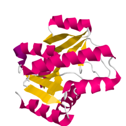
Figure 2: An example protein structure. The secondary structure elements are the alpha helices and the beta strands (represented by arrows); the strands can be seen to lie in parallel to form structures called beta sheets.

In this paper, we describe a fully Bayesian model for the alignment of proteins using structural information in the form of atomic coordinates of the amino acids, and hence the problem is one of statistical shape analysis (in particular, unlabelled shape analysis (e.g. Green and Mardia, (2006); Dryden and Mardia, (2016); Rodriguez and Schmidler, (2014)). We use sequence order in the modelling, in the sense that the sequence order information forms the basis of our prior distribution over all possible alignments, through the use of gap penalty functions. (Note however that our model can also easily incorporate other sources of sequence information, such as amino acid type.) Our prior distribution uses a penalty function of very general form, and hence the framework allows for a very rich and flexible class of prior distributions which can capture desirable features of an alignment. The framework allows the use of a penalty function commonly used in bioinformatics as a special case, on which Rodriguez and Schmidler, (2014) based their prior distribution on alignments. However, this penalty function has some undesirable properties, and its widespread use can arguably be attributed to its simplicity and ease of computational implementation rather than its biological realism. Here, we propose one possible penalty function which fits into our general framework, motivated by a desirable “proportionality” property (see Section 3.3) which is very natural and plausible biologically. We note that there are many other possibilities which fit into this framework, and hence our model could be used in other contexts, with penalties chosen to capture particular desirable features related to the problem at hand.

The key ingredients of our methodology are:

• A probability model for the atomic coordinates, conditional on a particular amino acid correspondence (alignment) and geometric transformation (Section 3.1).

• A prior distribution over all possible alignments which retain sequence order, based on a gap penalty function. We show how a general class of penalties fit into the framework (Section 3.2), and suggest a particular penalty function which addresses an intuitively undesirable feature of a popular penalty function (Section 3.3).

• A posterior distribution over all alignments and transformation parameters (Section 3.2), such that all sources of uncertainty are handled in a principled manner, allowing alternative alignments to be explored and their merits quantified probabilistically. In Section 3.4 we show how alignments can be sampled efficiently from the posterior distribution, and that other priors of a very general form could be incorporated in the same way.

1.2 Protein similarity measures

Once proteins have been aligned, it is often useful to quantify the similarity between them. These measures are also used to compare different alignments between the same proteins, and so optimising them can also be part of the alignment process. In this section, we discuss some of the issues in quantifying protein structure similarity, and some of the measures which have been proposed to do so.

Consider two proteins $\bm{X}$ and $\bm{Y}$ with $m$ and $n$ residues respectively. Suppose $L$ residues have been aligned, where $\{\bm{x}_{i}\}_{i=1}^{L}$ and $\{\bm{y}_{i}\}_{i=1}^{L}$ are the atomic coordinates of these points on $\bm{X}$ and $\bm{Y}$ respectively. A basic measure of similarity is the root mean squared deviation (RMSD), given by

$$\sqrt{\frac{1}{L}\displaystyle\sum_{i=1}^{L}||\bm{x}_{i}-\bm{A}\bm{y}_{i}-\bm{\tau}||^{2}},$$

where $\bm{A}$ is the rotation matrix and $\bm{\tau}$ the translation vector giving the optimal superposition of $\bm{Y}$ on $\bm{X}$. A problem with interpreting RMSD as an absolute measure of similarity is that longer alignments (larger $L$) tend to have larger RMSD. Since long alignments and low RMSD are both desirable, there is a trade-off between choosing a longer alignment and smaller RMSD. This also makes comparing different alignments (e.g. those from different methods) difficult, unless one is Pareto optimal (longer alignment and smaller RMSD). In the Matt algorithm, Menke et al., (2008) and Daniels et al., 2012a considered the balance of RMSD and $L$ as a proxy for homology, and found a linear combination of the two measures which achieved optimal performance on a particular benchmark data set, SABmark (Van Walle et al., , 2005), in terms of separating homologous proteins at superfamily level from decoys.

Two measures which have been proposed as more general and robust measures of similarity are Global Template Score (GDT) (Zemla, , 2003) and Template Modelling (TM) score (Zhang and Skolnick, , 2004). GDT is defined as

$$100\frac{(n_{1}+n_{2}+n_{4}+n_{8})}{4L},$$

where $n_{a}$ is the (cumulative) number of aligned residues which are less than $a~{}\mbox{\AA}$ apart after superposition of the proteins. TMscore is defined as

$$\frac{1}{m}\displaystyle\sum_{i=1}^{L}\frac{1}{1+(\frac{d_{i}}{d_{0}})^{2}},$$

where $d_{0}=1.24\sqrt[3]{m-15}-1.8$, $d_{i}$ is the distance between the $i^{\rm{th}}$ pair of residues after superposition, and $m$ is the total number of residues on the smaller protein. The parameter $d_{0}$ provides a scale for normalising distances, and the TMscore was designed to improve upon measures of the same form, but which use constant values of $d_{0}$, such as $3.5$ or $5$. For measures which use a fixed value of $d_{0}$, Zhang and Skolnick, (2004) found a power law relationship between measurement scores and length (of the smaller protein) for randomly-chosen protein pairs with $<30\%$ sequence similarity. The value of $d_{0}$ used in TMscore depends on the length of the smaller protein, and was found to correct the observed bias towards longer proteins in other measures.

1.3 Review of existing methods

Here, we briefly review the main approaches for representing, and some of the algorithms developed for aligning, protein structures. The list is far from exhaustive, and we focus on covering the main approaches and some of the most well-known/popular methods. For a review of the main ideas and approaches to structure alignment, see Hasegawa and Holm, (2009) and Ma and Wang, (2014), who also give a comprehensive account of the available methods and discuss some open challenges.

The most common representations of protein structures used in pairwise structure comparison methods are as sets of points, distance matrices, or secondary structure elements. The first approach represents the protein by a set of atomic coordinates, typically the $C_{\alpha}$ (alpha-carbon) atoms (which is also the approach we adopt in this paper). The second approach uses a matrix of intra-protein distances, such as the matrix of distances between $C_{\alpha}$ atoms. The final approach uses SSEs (alpha helices and beta strands). Some methods use a combination of these, or incorporate additional knowledge such as amino acid type and hydrogen bonding information.

TMalign (Zhang and Skolnick, , 2005), LGA (Zemla, , 2003), Matt (Menke et al., , 2008), FATCAT (Ye and Godzik, , 2003) and DeepAlign (Wang et al., , 2013) are examples of methods using the point set representation. TMalign and LGA consider rigid-body motions in order to establish an optimal alignment. Matt and FATCAT consider flexibility in the proteins by identifying fragments of structure, with “bends” allowed between the fragments. Formatt (Daniels et al., 2012b, ) builds on Matt by including amino acid sequence information to refine structural alignments. DeepAlign also utilises additional information from the amino acid sequence, as well as hydrogen bonds and local substructure substitution scores. DALI (Holm and Sander, , 1993) uses the distance matrix representation, and CE (Shindyalov and Bourne, , 1998) uses a combination of atomic locations and distances. The VAST algorithm (Gibrat et al., , 1997) uses the SSEs, represented as vectors.

Computational methods such as these seek to optimise some heuristically-justified scoring function, with the optimisation taking place over amino acid correspondences and/or some form of geometrical superposition. In this paper, we introduce a fully probabilistic model which incorporates all sources of uncertainty in a principled manner, allowing alternative alignments to be explored and their merits quantified probabilistically.

The overall structure of the paper is as follows. In Section 2 we formulate the problem as one of unlabelled shape analysis, and briefly discuss some alternative statistical methods. In Section 3, we describe the Bayesian model for structural alignment, and give details of our new prior distribution over alignments. In Section 4 we apply our method to some challenging examples and benchmark data sets, and compare with some popular structural alignment methods, before concluding with a discussion.

2 Mathematical formulation: unlabelled shape analysis

In this section, we formulate the problem as one of (unlabelled) statistical shape analysis, and review some of the relevant literature in this area.

Mathematically, a protein can be represented as a configuration of $m$ points, $\{\bm{x}_{j}\}_{j=1}^{m}$, $\bm{x}_{j}\in\mathbb{R}^{3}$. For example, the points often represent the locations of the $C_{\alpha}$ (alpha-carbon) atoms of the amino acids. The problem is then to align this configuration with that of another protein $\{\bm{y}_{k}\}_{k=1}^{n}$. That is, we seek a rigid body transformation such that

$$\bm{A}\bm{y}+\bm{\tau}=\bm{x}$$

for any pair of points $\bm{x}$ and $\bm{y}$ which are “matched” — i.e. $\bm{x}$ and $\bm{y}$ are equivalent points on their respective configurations. Here, $\bm{A}$ is a $3\times 3$ rotation matrix and $\bm{\tau}\in\mathbb{R}^{3}$ is a translation vector. The correspondence between points on the two configurations is encoded in an $m\times n$ matrix $\bm{M}$, with elements $M_{jk}$, where

$M_{jk}=\left\{\begin{array}[]{cc}1,&\textrm{if}\hskip 5.69046pt\bm{x}_{j}\hskip 5.69046pt\textrm{and}\hskip 5.69046pt\bm{y}_{k}\hskip 5.69046pt\textrm{are matched,}\\ 0,&\textrm{otherwise.}\end{array}\right.$

Usually, $\bm{M}$ is not known and it is the main object of interest about which to draw inference; this is known as unlabelled shape analysis, and the problem of protein structure alignment is an important example of this.

Unlabelled shape analysis has been the focus of much recent research interest in statistical shape analysis, motivated by important applications such as that of protein structure alignment. From the Bayesian viewpoint, there are essentially two approaches that have been developed for unlabelled shape analysis. One approach is to maximize over the transformation parameters $\bm{A}$ and $\bm{\tau}$ (Dryden et al., , 2007; Schmidler, , 2007; Rodriguez and Schmidler, , 2014) which can be viewed as using a Laplace approximation to integrate out $\bm{A}$ and $\bm{\tau}$ and using the marginal posterior distribution for inference about $\bm{M}$ (Kenobi and Dryden, , 2012). An alternative approach is to consider a fully Bayesian model, where the transformation parameters are included as unknown parameters in the model about which to draw inference (Green and Mardia, , 2006). In this manner, uncertainty in these parameters is accounted for and correctly propagated throughout the analysis (Wilkinson, , 2007). Other approaches to the unlabelled shape alignment problem include the Softassign Procrustes method of Rangarajan et al., (1997) and methods using the EM algorithm (Kent et al., , 2010; Myronenko and Song, , 2010). A closely-related problem is that of looking for instances of a known shape in cluttered point clouds, for example searching for shapes in noisy images (Srivastava and Jermyn, , 2009; Su et al., , 2013).

An alternative description of a protein useful for statistical modelling is as a sequence of pairs of dihedral angles defined by the backbone of a protein, with each pair a point on a torus. For example, Boomsma et al., (2008) used hidden Markov models as generative models for protein structure. Lennox et al., (2009) use Dirichlet process mixtures for density estimation of the distribution of dihedral angles, a problem also considered by Maadooliat et al., (2016) using nonparametric density estimation, focussing on modelling loop regions of a protein; see also Najibi et al., (2017). Motivated by direct modelling of the evolution of a protein, Golden et al., (2017) describe the shape of a protein as a sequence of dihedral angles on the torus; their model captures dependencies between sequence and structure evolution through a diffusion process on the torus.

In this paper, we consider the alignment of protein structures within the fully Bayesian framework of Green and Mardia, (2006), but with an important change to the prior model for the matching matrix $\bm{M}$. In the original setting of Green and Mardia, (2006), conditional on the total number of matched points $L$, then every possible $\bm{M}$ consistent with $L$ matched points was considered equally likely. When aligning homologous proteins which are thought to have evolved from a common ancestor, it is important to preserve the sequence order of the points in the matching given by $\bm{M}$. Therefore, we require a prior for $\bm{M}$ which imposes this constraint. This has previously been considered by Rodriguez and Schmidler, (2014), who worked out in detail the case corresponding to a prior based on a commonly-used penalty function in bioinformatics, which they used in their applications; they also suggested that more general priors, applicable in other situations, could be incorporated in this framework. We introduce a class of priors based on a more general penalty function, which alleviates the unappealing feature that, conditional on the numbers of matches and gaps, the indices of the points forming the matches are independent under the prior model. We show how this new prior can be incorporated into the fully Bayesian framework of Green and Mardia, (2006), and how an MCMC scheme can be implemented in light of the changes to the model due to this prior. (See also Mardia, (2013), who considered alignment preserving sequence order, but with a uniform prior over all possible such alignments.) This methodology can give biologically-meaningful alignments on challenging problems, as well as accounting for uncertainty in the alignment and transformation parameters in a fully Bayesian manner.

The underlying formulation is very flexible. For instance, Green and Mardia, (2006) considered rigid body transformations in their applications, but Mardia et al., (2013) demonstrated applications using full similarity transformations. Forbes et al., (2014) also use this approach with similarity transformations in the context of fingerprint matching. Green, (2015) describes how the MAD-Bayes technique (Broderick et al., , 2013) can be used to obtain approximations to the MAP (maximum a-posteriori) estimator, useful when very fast approximate solutions might be needed in practical situations using very large data sets, a problem also considered by Schmidler, (2007).

3 Bayesian structure alignment

We now describe our Bayesian model for protein structure alignment. In Section 3.1 we form the likelihood, and in Section 3.2 describe a general form of prior distribution on alignments based on gap penalty functions, showing how a commonly-used penalty is a special case. In Section 3.3, a new prior for the matching matrix $\bm{M}$ is proposed, which alleviates an undesirable property of the aforementioned common penalty function. In Section 3.4, we detail our sampler for drawing samples from the posterior distribution of alignments, and in Section 3.5 describe how a point estimate alignment is obtained.

3.1 Likelihood

We have two point configurations, $\bm{X}=\{\bm{x}\}$ and $\bm{Y}=\{\bm{y}\}$, consisting of $m$ and $n$ points respectively. The points are labelled $\bm{x}_{j},\hskip 5.69046ptj=1,\ldots,m$ and $\bm{y}_{k},\hskip 5.69046ptk=1,\ldots,n$, where $\bm{x}_{j},\hskip 5.69046pt\bm{y}_{k}\in\mathbb{R}^{d}$; in our case, protein structures are $3$-dimensional configurations and $d=3$. A rigid body transformation which transforms points on $\{\bm{y}\}$ into $x$-space is of the form $\bm{A}\bm{y}+\bm{\tau}$, where $\bm{A}$ is a $d\times d$ rotation matrix and $\bm{\tau}\in\mathbb{R}^{d}$ is a translation vector. As in Green and Mardia, (2006), we have

$$\bm{x}_{j} = \bm{\mu}_{\xi_{j}}+\bm{\epsilon}_{j}\hskip 5.69046pt\hskip 5.69046ptj=1,\ldots,m,$$

$$\bm{A}\bm{y}_{k}+\bm{\tau} = \bm{\mu}_{\eta_{k}}+\bm{\epsilon}_{k}\hskip 5.69046pt\hskip 5.69046ptk=1,\ldots,n,$$

where $\{\bm{\mu}\}$ is an unobserved hidden configuration, from which the observed points are derived. The $\bm{\epsilon}$ terms represent error in the observed points, which are regarded as noisy observations of the true locations on $\{\bm{\mu}\}$. Here, we use a spherical Gaussian model for the errors, so that $\bm{\epsilon}\sim N_{d}(0,\sigma^{2}\bm{I})$, where $\bm{I}$ is the $d\times d$ identity matrix; the parameter $\sigma^{2}$ therefore represents the error variance. The $\xi$ and $\eta$ terms give the mapping between points on $\{\bm{\mu}\}$ and points on $\{\bm{x}\}$ and $\{\bm{y}\}$ respectively. In particular, when $\xi_{j}=\eta_{k}$ then the corresponding $\bm{x}$ and $\bm{y}$ points are both realisations of the same hidden location, and are regarded as matched points. The matching between the configurations is captured by the matching matrix $\bm{M}$. We impose the constraint that a given point on one configuration can match at most one point on the other configuration, so that each row or column of $\bm{M}$ has at most one non-zero entry. Then, $\displaystyle\sum_{j,k}M_{jk}=L$, where $L$ is the total number of matched pairs of points.

The points on $\{\bm{\mu}\}$ are assumed to form a homogeneous Poisson process over a region of volume $v$, and these hidden points can be integrated out. Then, assuming $v$ is large relative to the support of the density of the error terms, the (approximate) respective likelihood contributions of the unmatched $\bm{x}$, unmatched $\bm{y}$ and matched points are

$$v^{-(m-L)},\hskip 5.69046pt(|\bm{A}|/v)^{n-L},\hskip 5.69046pt(|\bm{A}|/v)^{L}\displaystyle\prod_{j,k:M_{jk}=1}\frac{\phi\{(\bm{x}_{j}-\bm{A}\bm{y}_{k}-\bm{\tau})/(\sigma\sqrt{2})\}}{(\sigma\sqrt{2})^{d}},$$

where $\phi(\cdot)$ is the $d$-dimensional standard normal density. Hence the likelihood of the observed data given $\bm{M}$ (and the other parameters) is

$$p(\bm{x},\bm{y}|\bm{M},\bm{A},\bm{\tau},\sigma)=v^{-(m+n-L)}|\bm{A}|^{n}\displaystyle\prod_{j,k:M_{jk}=1}\frac{\phi\{(\bm{x}_{j}-\bm{A}\bm{y}_{k}-\bm{\tau})/(\sigma\sqrt{2})\}}{(\sigma\sqrt{2})^{d}}.$$ (1)

3.2 Gap prior

Recall that our main objective is to align two configurations when the points on each configuration have a meaningful ordering which must be preserved in any resulting alignment, which may include gaps in the corresponding sequence alignment in one or both of the sequences. We summarise an alignment with the matching matrix $\bm{M}$, for which we use a prior which imposes the sequence order constraint. As a starting point, we use the prior

$$p(\bm{M};g,h)=Z(g,h)\exp\{-u(\bm{M};g,h)\},$$ (2)

as in Rodriguez and Schmidler, (2014), where $u(\bm{M};g,h)$ is a penalty function which penalises gaps in the alignment, and $Z(g,h)$ is a normalising constant. The parameters $g$ and $h$ are known as gap opening and extension penalties respectively. The penalty function is

$$u(\bm{M};g,h)=gs(\bm{M})+hl(\bm{M})$$ (3)

where $s(\bm{M})$ is the number of instances where a new gap in the alignment is opened, $l(\bm{M})=\sum_{i=1}^{S(\bm{M})}(l_{i}-1)$, and $l_{i}$ is the length of the $i$th gap. This corresponds to a gap penalty function widely used in sequence alignment (Durbin et al., , 1998). The prior (2) using penalty function (3) was used by Liu and Lawrence, (1999) in a Bayesian sequence alignment setting. Wu et al., (1998) also used the penalty (3), in what we believe to be the first statistical work on protein sequence and structure alignment, which was set in a regression framework.

To illustrate what is meant by a new gap and length of a gap, consider again the sequence alignment in Figure 1 (b). In the first sequence, the second residue is not matched to a residue on the second sequence; instead it is aligned to a “-”, indicating that a gap has been opened. That is, a gap opening is said to have been created where a residue in one sequence is unmatched, but the previous residue in the same sequence was aligned to a residue in the other sequence. The length of the gap is then the number of unmatched residues (in the same sequence) until another matched pair; therefore, the gap in Figure 1 (b) is of length $3$.

In Figure 1 (c), the first sequence has one gap, of length $1$, and the second sequence has three gaps, of lengths $1$, $2$ and $1$. Note that the two sequences are considered independently when counting the number and length of the gaps, so that a gap in one sequence followed immediately by a gap in the other sequence would be counted as two different gap openings.

Before introducing a generalisation of the prior distribution (2), we first illustrate how this prior fits into our framework. Recall that configurations $\bm{X}$ and $\bm{Y}$ consist of $m$ and $n$ points respectively, and suppose that there are $L$ matched points between the two. Further, suppose the indices of the matched points on $\bm{X}$ are $j_{0}<j_{1}<j_{2}<\cdots<j_{L}<j_{L+1}$ and the indices of the matched points on $\bm{Y}$ are $k_{0}<k_{1}<k_{2}<\cdots<k_{L}<k_{L+1}$. Hence, if $j_{i+1}-j_{i}\geq 2$, there is a gap in the $\bm{X}$ sequence of length $j_{i+1}-j_{i}-1$, and similarly for $\bm{Y}$ involving the $k$ indices. We set $j_{0}=k_{0}=0$ and $j_{L+1}=m+1$, $k_{L+1}=n+1$, which are artificial matching indices, fixed throughout, introduced to account for the start and end points of the sequences.

Hence, the total penalty given by (3) is

$$u(\bm{M};g,h)=\displaystyle\sum_{i=0}^{L}f(j_{i+1}-j_{i})+\displaystyle\sum_{i=0}^{L}f(k_{i+1}-k_{i}),$$

where

$$f(r)=\left\{\begin{array}[]{cc}0&\hskip 11.38092ptr=1\\ g&\hskip 11.38092ptr=2\\ g+(r-2)h&\hskip 11.38092ptr>2.\\ \end{array}\right.$$

Thus, the total penalty can be easily computed as a sum of simple contributions involving consecutive pairs of the matched point indices. In the same spirit, we can generalise the prior distribution (2) by incorporating other penalty functions $u(\bm{M};\bm{\phi})$ which are expressible as a sum of penalty contributions involving small subsets of the matching indices. Here, $\bm{\phi}$ is a vector of parameters, and in the special case (3), we have $\bm{\phi}=(g,h)$. This has positive implications for the implementation, as follows. The MCMC sampling methods we employ (described in Section 3.4) involve computing differences of the form $u(\bm{M}^{\prime};\bm{\phi})-u(\bm{M};\bm{\phi})$, where $\bm{M}^{\prime}$ is a proposed modification of $\bm{M}$. The computation will be efficient if the change from $\bm{M}$ to $\bm{M}^{\prime}$ only affects a small number of the terms which comprise $u(\bm{M};\bm{\phi})$, and each of these terms are simple to compute. We describe a novel penalty function in Section 3.3 that adheres to this principle, which corresponds to a prior which can control the degree of “proportionality” in the indices of the matched points.

Since we are using a different form of prior distribution on $\bm{M}$ to that considered by Green and Mardia, (2006), there is a minor change to the joint model (Equation (6) in that paper). As described above, the priors we consider are of the general form

$$p(\bm{M};\bm{\phi})\propto\exp\{-u(\bm{M};\bm{\phi})\}.$$ (4)

Multiplying (1) and (4), we obtain

$$p(\bm{M},\bm{x},\bm{y}|\bm{A},\bm{\tau},\sigma)\propto|\bm{A}|^{n}v^{L}\exp\{-u(\bm{M};\bm{\phi})\}\displaystyle\prod_{j,k:M_{jk}=1}\frac{\phi\{(\bm{x}_{j}-\bm{A}\bm{y}_{k}-\bm{\tau})/(\sigma\sqrt{2})\}}{(\sigma\sqrt{2})^{d}}$$

and the joint model is

$$\begin{split}p(\bm{M},\bm{A},\bm{\tau},\sigma,\bm{x},\bm{y})&\propto p(\bm{A})p(\bm{\tau})p(\sigma)|\bm{A}|^{n}v^{L}\exp\{-u(\bm{M};\bm{\phi})\}\\ &\quad\times\displaystyle\prod_{j,k:M_{jk}=1}\frac{\phi\{(\bm{x}_{j}-\bm{A}\bm{y}_{k}-\bm{\tau})/(\sigma\sqrt{2})\}}{(\sigma\sqrt{2})^{d}}.\\ \end{split}$$ (5)

In particular, the term $v^{L}$ remains, unlike in the model of Green and Mardia, (2006), where this term cancelled with a corresponding term from the prior for $\bm{M}$. We discuss specification of $v$ in our applications in Section 4.1. The prior distributions on $\bm{A}$, $\bm{\tau}$ and $\sigma$ are $p(\bm{A}),p(\bm{\tau})$ and $p(\sigma)$ respectively. The rotation matrix $\bm{A}$ has a matrix-Fisher prior distribution, where $p(\bm{A})\propto\exp\left\{\mbox{tr}(\bm{F}_{0}^{T}\bm{A})\right\}$ and the parameter $\bm{F}_{0}$ is a $d\times d$ matrix. $\bm{A}$ is parametrised by Eulerian angles, $\theta_{12},\theta_{13},\theta_{23},$ say, in the case $d=3$. In our examples we use a uniform prior on $\bm{A}$, which is the special case where $\bm{F}_{0}$ is the $d\times d$ matrix of zeroes. $\bm{A}$ then has a uniform prior with respect to the invariant measure on $SO(3)$, the Haar measure, where $SO(3)$ is the special orthogonal group of all $d\times d$ rotation matrices. For the translation vector $\bm{\tau}$, we have $\bm{\tau}\sim N_{d}(\bm{\mu}_{\tau},\sigma_{\tau}^{2}\bm{I}_{d})$, where $\bm{\mu}_{\tau}$ is a mean vector and $\sigma_{\tau}^{2}\bm{I}_{d}$ a covariance matrix, with $\bm{I}_{d}$ the $d\times d$ identity matrix. For the noise parameter $\sigma$, we have $\sigma^{-2}\sim\Gamma(\alpha,\beta)$, so $p(\sigma^{-2})\propto\sigma^{-2(\alpha-1)}\exp\left(-\frac{\beta}{\sigma^{2}}\right)$.

3.3 A proportionality prior

We now describe our new penalty function, which controls “proportionality” in the alignment and contains the penalty in (3) as a special case.

Consider the pair of triples $(j_{1},j_{2},j_{3})$ and $(k_{1},k_{2},k_{3})$, from which we obtain the pair $(j_{2}-j_{1})$, $(j_{3}-j_{2})$ from the $\bm{X}$ sequence and the pair $(k_{2}-k_{1})$ , $(k_{3}-k_{2})$ from the $\bm{Y}$ sequence. Given $j_{1},j_{3},k_{1},k_{3}$, we would prefer $j_{2}$ and $k_{2}$ such that the ratio

$$\frac{(j_{2}-j_{1})/(j_{3}-j_{2})}{(k_{2}-k_{1})/(k_{3}-k_{2})}$$

is close to one.

In general, given $L$ matches, we have $L$ triples of matching indices in the $\bm{X}$ sequence, given by
$(j_{0},j_{1},j_{2}),(j_{1},j_{2},j_{3}),\ldots,(j_{L-1},j_{L},j_{L+1})$. Similarly, in the $\bm{Y}$ sequence we have the $L$ triples $(k_{0},k_{1},k_{2}),(k_{1},k_{2},k_{3}),\ldots,(k_{L-1},k_{L},k_{L+1})$. For the $i$th pair of triples, consider the log ratio

$$q_{i}=\log\left\{\frac{(j_{i}-j_{i-1})/(j_{i+1}-j_{i})}{(k_{i}-k_{i-1})/(k_{i+1}-k_{i})}\right\}.$$

Then a Gaussian-type penalty on the lack of proportionality is given by

$$\gamma(q_{i};\nu)=\frac{\nu q_{i}^{2}}{2}.$$

Combining this with the penalty function (3) (which uses only $s(\bm{M})$ and $l(\bm{M})$), the total penalty function is

$$u(\bm{M};g,h,\nu)=gs(\bm{M})+hl(\bm{M})+\displaystyle\sum_{i=1}^{L}\gamma(q_{i};\nu).$$

Letting $\nu=0$, we obtain the original penalty (3).

For example, consider the case with $m=8$, $n=17$ and $L=3$. Two possible alignments ($\bm{M}_{1}$ and $\bm{M}_{2}$ respectively say) are

$$\begin{array}[]{cccccc}\bm{M}_{1}:&j_{0}&j_{1}&j_{2}&j_{3}&j_{4}\\ &0&2&5&7&9\\ &0&4&10&14&18\\ &k_{0}&k_{1}&k_{2}&k_{3}&k_{4}\end{array}$$

and

$$\begin{array}[]{cccccc}\bm{M}_{2}:&j_{0}&j_{1}&j_{2}&j_{3}&j_{4}\\ &0&2&5&7&9\\ &0&2&12&16&18\\ &k_{0}&k_{1}&k_{2}&k_{3}&k_{4}\end{array}$$

In both cases, $s(\bm{M})=8$ and $l(\bm{M})=11$ and hence the original gap penalty is the same, so $p(\bm{M}_{1};g,h)/p(\bm{M}_{2};g,h)=1$ under the original gap penalty prior.

Consider now the prior with the penalty for lack of proportionality included. For $\bm{M}_{1}$, we have $q_{1}=q_{2}=q_{3}=0$ (all ratios are equal to $1$). This gives a total penalty of $8g+11h$, the same as the original gap penalty. For $\bm{M}_{2}$ we have :

$$\begin{array}[]{c}q_{1}=\log\left\{\frac{(j_{1}-j_{0})/(j_{2}-j_{1})}{(k_{1}-k_{0})/(k_{2}-k_{1})}\right\}=\log\left(\frac{2/3}{2/10}\right)=1.204.\end{array}$$

With $\nu=1$, this gives a penalty of $\gamma(1.204;1)=0.5\times 1.204^{2}=0.725$ for the first pair of triples. Similarly, $q_{2}=\log(0.60)=-0.511$, giving a penalty of $0.131$, and $q_{3}=\log(0.5)=-0.693$, resulting in a penalty of $0.240$. The total penalty is

$$8g+11h+0.725+0.131+0.240=8g+11h+1.096.$$

Hence, under the new prior, $p(\bm{M}_{1};g,h,\nu)/p(\bm{M}_{2};g,h,\nu)=\exp(1.096)=2.99$.

Note that larger values of $\nu$ penalise a lack of proportionality more. For instance, in the example above with $\nu=4$ we have

$$\frac{p(\bm{M}_{1};g,h,\nu)}{p(\bm{M}_{2};g,h,\nu)}=\exp(4.38)=80$$

under the new prior, so $\bm{M}_{1}$ (which preserves proportionality perfectly) is strongly preferred over $\bm{M}_{2}$.

3.4 Sampling $\bm{M}$

Updates for the parameters $\bm{A}$, $\bm{\tau}$ and $\sigma$ are as in Green and Mardia, (2006). We now describe the mechanism for generating posterior samples of $\bm{M}$, using Metropolis-Hastings updates. Suppose our current alignment is $\bm{M}$, and we have a proposal value $\bm{M}^{{}^{\prime}}$ drawn from a proposal density $q(\bm{M}^{{}^{\prime}};\bm{M})$. Then the acceptance probability is

$$\alpha=\mbox{min}\left\{1,\frac{p(\bm{M}^{{}^{\prime}},\bm{A},\bm{\tau},\sigma,\bm{x},\bm{y})q(\bm{M};\bm{M}^{{}^{\prime}})}{p(\bm{M},\bm{A},\bm{\tau},\sigma,\bm{x},\bm{y})q(\bm{M}^{{}^{\prime}};\bm{M})}\right\},$$

where $p(\cdot)$ is the joint model (5).

Similar to Green and Mardia, (2006), we consider three types of update for $\bm{M}$, namely adding a matched pair, deleting a matched pair, or switching a matched pair, but the form of the updates is different due to the new prior on $\bm{M}$. We illustrate the idea by considering adding a matched pair, and the other two cases are similar; full details of our sampler are given in supplementary information. Suppose there are currently $L$ matches with indices $j_{1}<j_{2}<\cdots<j_{L}$ and $k_{1}<k_{2}<\cdots<k_{L}$. Suppose further that we propose to add a match ($j^{*}$,$k^{*}$), where $j_{i}<j^{*}<j_{i+1}$ and $k_{i}<k^{*}<k_{i+1}$, $i=0,\ldots,L$, and we also have $j_{0}=k_{0}=0$ and $j_{L+1}=m+1,k_{L+1}=n+1$. Then

$$\frac{p(\bm{M}^{{}^{\prime}},\bm{A},\bm{\tau},\sigma,\bm{x},\bm{y})}{p(\bm{M},\bm{A},\bm{\tau},\sigma,\bm{x},\bm{y})}=\exp\{u(\bm{M};\bm{\phi})-u(\bm{M}^{{}^{\prime}};\bm{\phi})\}\times\frac{v\phi\{(\bm{x}_{j^{*}}-\bm{A}\bm{y}_{k^{*}}-\bm{\tau})/(\sigma\sqrt{2})\}}{(\sigma\sqrt{2})^{d}},$$

where $u(\bm{M};\bm{\phi})-u(\bm{M}^{{}^{\prime}};\bm{\phi})$ is the reduction in the gap penalty achieved by adding the match ($j^{*}$,$k^{*}$). As described in Section 3.2, the penalty functions we consider are of a form which facilitates efficient computation of this reduction; since only a small number of terms involving matched indices either side of ($j^{*}$,$k^{*}$) are affected, it is not necessary to recalculate the whole penalty each time a change to $\bm{M}$ is proposed.

Note that under this sampling method, we make only small perturbations to the alignment at each iteration, by either removing a match, adding a match, or switching a match, so that the total number of matches can change by at most $1$. Our sampler is quite simple compared to that used by Rodriguez and Schmidler, (2014), who propose global changes to $M$ using dynamic programming recursions analogous to those used in sequence alignment algorithms (Zhu et al., , 1998; Liu and Lawrence, , 1999), which may improve performance. Instead, we improve performance of our sampler, which makes local changes to $M$, using parallel tempering (Geyer, , 1991).

3.5 Point estimation

As described in Green and Mardia, (2006), the principles of Bayesian decision theory can be used to obtain a posterior point estimate for $\bm{M}$ from our MCMC output, by defining a loss function which incorporates costs for falsely declaring matches and missing true matches. It is necessary only to specify a value for a parameter $K$, where $K=c_{01}/(c_{01}+c_{10})$; the term $c_{01}$ denotes the cost incurred for falsely declaring a match, and $c_{10}$ denotes the cost of falsely missing a true match. The point estimate is obtained by minimising the expected loss with respect to the marginal posterior matching probabilities, which can be regarded as a linear assignment problem. Note that larger values of $K$ give fewer matches, since falsely declaring a match incurs a relatively higher cost than missing a true match. As a default, we take $K=0.5$, so that both types of error are considered equally costly. To solve the linear assignment problem, we use the method of Jonker and Volgenant, (1987).

4 Applications

We now illustrate our methodology with applications to real protein data. We first analyse the pair of proteins with PDB identification codes 1GKY and 2AK3, also analysed by Rodriguez and Schmidler, (2014), which have been studied previously in the structural bioinformatics literature. We then investigate the performance of our method on a set of $16$ protein pairs considered to be challenging for structural alignment methods (Jung and Lee, , 2000; Ortiz et al., , 2002), which Rodriguez and Schmidler, (2014) used to compare their method against the CE algorithm of Shindyalov and Bourne, (1998). We then present results on the MALIDUP and RIPC benchmark data sets, and compare with some of the available methods from computational biology. In all cases, we find that our results are competitive with these other methods.

4.1 Parameter settings

It is necessary to specify a value of the parameter $v$, which represents the volume of the region in which the configurations of points are realised. We specify $v$ as follows. Let $\bar{\Omega}_{x}=\prod_{i=1}^{3}\{\max_{j}(x_{ji})-\min_{j}(x_{ji})\}$ be the volume of the region containing the $\bm{X}$ configuration. Similarly, let $\bar{\Omega}_{y}=\prod_{i=1}^{3}\{\max_{k}(y_{ki})-\min_{k}(y_{ki})\}.$ Then define $\bar{\Omega}=\max\{\bar{\Omega}_{x},\bar{\Omega}_{y}\}.$ As a default, we take $v=1.2\bar{\Omega}$, which is the value used for the reported results. We found our results to be robust to increases in this parameter.

The parameter settings we used for the user-defined parameters which remain fixed throughout this section are summarized in Table 1. We use the values $g=4$ and $h=0.1$ for the gap opening and extension penalty parameters, reflecting that the opening of a gap should be penalised more than extending a gap, to discourage alignments with lots of short gaps which are not plausible biologically (Altschul, , 1988). The values we use are equal to the expected values of $g$ and $h$ from the prior distributions used by Rodriguez and Schmidler, (2014), who suggest that a gap opening penalty of the order of $40$ times as large as the gap extension penalty is reasonable, following Gerstein and Levitt, (1998). For the parameter $\nu$, we compare the results obtained using the values $0.25$ and $4.0$ in order to assess the effect of our new prior on the resulting alignments. We chose these values after numerical experimentation using simulations from the prior distribution on $M$; we found $\nu=4.0$ encourages proportionality very strongly, to the point where this excessively dominates the gap opening and extension penalties, whereas a value of $\nu=0.25$ gave a more even balance between proportionality and gaps. More details, including plots of simulations from the prior, are given in the supplementary material.

Table 1: Parameter settings for user-defined parameters which remain fixed.

$g$	$h$	$\beta$	$\sigma_{\tau}$
$4$	$0.1$	$8$	$500$

For the remaining parameters, we use the following settings. The prior mean for the translation, $\bm{\mu}_{\tau}$, is taken to be the difference between the centroids of the two configurations. Prior information on $\bm{\tau}$ is weak, so we set $\sigma_{\tau}=500$ to give a diffuse prior to reflect this. The prior for the rotation matrix $\bm{A}$ is uniform. We set $\alpha=1$, giving an exponential prior for $\sigma^{-2}$ with mean $1/\beta$. We keep $\beta=8$ fixed throughout, corresponding to a mean precision broadly similar to the resolutions typical of PDB data (around $1$–$3$ Å) — posterior inferences are robust to moderate changes of this value for $\beta$. The initial matching matrix $\bm{M}$ was taken to be the zero matrix, corresponding to no matched points. All results relating to a specific alignment were obtained using the point estimate of $M$ with $K=0.5$, as discussed in Section 3.5, which means false negative and false positive matches are equally undesirable.

With unlabelled shape analysis in general, the posterior distribution is known to be inherently multimodal, with the potential for MCMC samplers to become trapped in subsidiary modes (Dryden et al., , 2007; Rodriguez and Schmidler, , 2014) corresponding to poor alignments. There may also be more than one genuinely-interesting mode, corresponding to different alignments of biological interest, and a strength of the Bayesian approach is the potential ability to explore the full posterior distribution and quantify the relative merits of each. To help ensure good convergence and mixing properties of the sampler, we used the parallel tempering method (Geyer, , 1991), with $N=6$ chains at temperatures $T_{1}<T_{2}<\cdots<T_{6}$, where $T_{1}=1$ is the chain corresponding to the target posterior distribution and we used $T_{6}=32$. For the remaining temperatures, the following scheme was used: $T_{i}=(1/T_{i+1}+\Delta)^{-1},i=2,\ldots,5$, where $\Delta=(1-1/T_{6})/(N-1)$. This scheme was found via experimentation to perform well. Multiple chains were then run from different starting values for the parameters $\bm{A}$, $\bm{\tau}$ and $\sigma$, and posterior trace plots of the various parameters, as well as the log-posterior, were inspected visually.

4.2 Example

We first discuss alignment of the pair 1GKY (chain A, $186$ points) and 2AK3 (chain A, $226$ points). These are both kinases (enzymes which catalyze phosphorylation reactions); 1GKY in yeast and 2AK3 in cows. The proteins have a low sequence identity (percentage of aligned pairs which are the same amino acid residue type) (Zhu et al., , 1998), but are structural homologues (i.e. the proteins have evolved from a common ancestor) and are VAST structural neighbours (Zhu et al., , 1998; Gibrat et al., , 1997); hence, a structural alignment can detect this relationship, despite the low sequence similarity. We compare alignments obtained using two different values of $\nu$, namely $\nu=0.25$ (prior mean number of matches approximately $158$) and $\nu=4.0$ (prior mean number of matches approximately $148$).

Since the configurations contain $m$ and $n$ points, the array of pairwise posterior matching probabilities is of dimension $m\times n$. However, this array will be rather sparse, with the non-negligible probabilities concentrated around the diagonal due to the sequence order constraint. In order to display an alignment, we plot the posterior matching probabilities of pairs for which the probability exceeds $0.001$, and the axes are linear combinations of the indices chosen to clearly display the diagonal region of interest. Figure 3 shows such displays for the two values of $\nu$ used. Each vertical segment corresponds to a matched pair, with the corresponding matching probability given by the length of the segment, the scale of which is indicated in the margin. The axes indicate the directions of increasing $\bm{X}$ (1GKY) and $\bm{Y}$ (2AK3) indices. For example, the regions marked A and B in Figure 3 (a) indicate longer sections where points in 1GKY are not aligned to any points in 2AK3, and the region marked C indicates a longer section of unaligned 2AK3 points. Figure 3 (a) is a display of the matching probabilities for the case $\nu=0.25$. We clearly see sections of low uncertainty in the alignment, corresponding to conserved regions of structure which can be aligned very well, as well as regions where there is more uncertainty. The point estimate $\hat{\bm{M}}$ (using $K=0.5$) consists of $152$ matched pairs of points and a corresponding RMSD of $3.0$.

Figure 3 (b) shows the corresponding plot with $\nu=4.0$. Comparing with the previous alignment ($\nu=0.25$), the alignments tend to agree where there was low uncertainty, with any differences being in more uncertain regions, such as those directly preceding and following the regions marked A and B. Additionally, there is a small section of aligned points introduced in the region marked C. In this case, the point estimate $\hat{\bm{M}}$ gives $153$ matched pairs of points and a corresponding RMSD of $3.2$. A value of $\nu=4.0$ penalises a lack of proportionality quite strongly — by the analogy with a Gaussian distribution used to construct the penalty in Section 3.3, $\nu$ is a precision parameter for the log ratio $q$, and $\nu=4.0$ corresponds to a standard deviation of $0.5$. Likewise, $\nu=0.25$ corresponds to a standard deviation of $2.0$. As a default, we use $\nu=0.25$, as used to obtain the following results presented in Sections 4.3, 4.4 and 4.5.

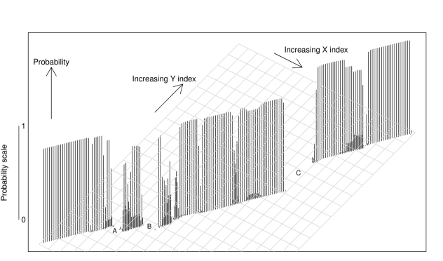
(a)

(b)

Figure 3: Posterior matching probabilities between pairs of points on proteins 1GKY ($X$) and 2AK3 ($Y$), with $\nu=0.25$ (a) and $\nu=4.0$ (b). The points are plotted in transformed coordinates to highlight the diagonal region of interest, where the horizontal coordinate is of the form $ax+by$ and the vertical coordinate is of the form $cy-dx$, where $x$ and $y$ are $X$/$Y$ indices and $c$ and $d$ are constants. The grid lines represent holding one of the original $X$/$Y$ coordinates fixed, with the direction of increasing $Y$/$X$ index indicated. The length of the vertical segment indicates the probability of the match between the corresponding pair of indices.

4.3 Comparison $1$: Ortiz et al., (2002) data set

We now present results on a set of $16$ pairs of proteins described by Jung and Lee, (2000) and further analysed in Ortiz et al., (2002). This set, which consists of protein pairs considered challenging for structural alignment methods, is used by Rodriguez and Schmidler, (2014) in their study. We shall refer to our method as SEQ-ALIBI (SEQuence-informed Alignment by Bayesian Inference), following ALIBI (Mardia, (2013); see also Green and Mardia, (2006)). We compare the results of SEQ-ALIBI (SA) with the method of Rodriguez and Schmidler, (2014), using the results reported for their parameter $\lambda=8.6$ (RS), and those from the CE algorithm of Shindyalov and Bourne, (1998), as reported by Rodriguez and Schmidler, (2014). The number of matches and corresponding RMSDs for each of the $16$ protein pairs are given in Table 2. We use the previously-suggested default values of $\nu=0.25$ and $K=0.5$, and values of all other parameters are set as described in Section 4.1. A comparison of the results obtained using various other combinations of $\nu$ and $K$ can be found in the supplementary material.

Table 2: RMSD and number of matches for the 16 protein pairs for CE, RS and SEQ-ALIBI.

		CE		RS		SEQ-ALIBI
Protein Pair	PDB IDs	RMSD	L	RMSD	L	RMSD	L
1	1ABA-1DSB	4.5	56	3.7	57	3.9	72
2	1ABA-1TRS	2.7	70	3.4	72	2.6	71
3	1ACX-1COB	4.0	92	3.8	86	2.7	84
4	1ACX-1RBE	7.3	56	2.8	31	4.3	52
5	1MJC-5TSS	2.7	61	3.0	60	2.3	60
6	1PGB-5TSS	2.9	48	3.3	55	2.7	55
7	1PLC-1ACX	3.3	80	4.0	84	2.8	73
8	1PTS-1MUP	4.1	80	3.1	83	2.8	85
9	1TNF-1BMV	4.1	115	4.2	109	3.7	112
10	1UBQ-1FRD	4.4	64	2.9	62	2.5	64
11	1UBQ-4FXC	4.0	64	2.9	61	2.6	64
12	2GB1-1UBQ	3.1	48	3.4	51	2.1	44
13	2GB1-4FXC	3.6	48	3.9	53	3.0	53
14	2RSL-3CHY	4.1	80	3.8	76	3.9	83
15	2TMV-256B	3.5	84	2.9	79	3.0	81
16	3CHY-1RCF	3.9	116	4.5	122	4.2	122

Table 3 summarizes the relative performance of CE and SEQ-ALIBI in terms of the trade-off between RMSD and number of matches. As discussed in Section 1.2, typically one is improved at the expense of the other, making comparisons of different alignments difficult. However, longer alignments with lower RMSD (Pareto optimality) are clearly desirable. For $8$ of the $16$ pairs, SEQ-ALIBI finds Pareto optimal alignments, and on no occasion is the reverse true.

Table 3: Comparison of number of matches ($L$) and RMSD between SEQ-ALIBI (SA) and CE for each of the $16$ protein pairs.

	Protein pair
$L^{\mbox{SA}}\geq L^{\mbox{CE}}$ and $\mbox{RMSD}^{\mbox{SA}}<\mbox{RMSD}^{\mbox{CE}}$	1 2 6 8 10 11 13 14
$L^{\mbox{SA}}\geq L^{\mbox{CE}}$ and $\mbox{RMSD}^{\mbox{SA}}>\mbox{RMSD}^{\mbox{CE}}$	16
$L^{\mbox{SA}}<L^{\mbox{CE}}$ and $\mbox{RMSD}^{\mbox{SA}}>\mbox{RMSD}^{\mbox{CE}}$	-
$L^{\mbox{SA}}<L^{\mbox{CE}}$ and $\mbox{RMSD}^{\mbox{SA}}<\mbox{RMSD}^{\mbox{CE}}$	3 4 5 7 9 12 15

Results from a similar comparison of SEQ-ALIBI with RS are given in Table 4. Again, there are $8$ cases where SEQ-ALIBI finds Pareto optimal alignments, and none where the reverse is true. The results from all $3$ methods for all $16$ protein pairs are plotted in Figure 4. For each pair, we have plotted RMSD against number of matches for each method, and drawn a line from the point for SEQ-ALIBI to the points for RS and CE. Near-vertical lines indicate an increase in RMSD for similar number of matches, and near-horizontal lines a reduction in matches for similar RMSD. Lines in a “north-west” direction signify the best performance of SEQ-ALIBI, since they indicate fewer matches and higher RMSD of the other method. Lines on the “south-west–north-east” axis correspond to pairs where neither method is clearly better, since more matches are being added at the cost of higher RMSD. Overall, we see that SEQ-ALIBI is at least as good as the other two methods, but does a lot better for some pairs.

Table 4: Comparison of number of matches ($L$) and RMSD between SEQ-ALIBI (SA) and RS for each of the $16$ protein pairs.

	Protein pair
$L^{\mbox{SA}}\geq L^{\mbox{RS}}$ and $\mbox{RMSD}^{\mbox{SA}}<\mbox{RMSD}^{\mbox{RS}}$	5 6 8 9 10 11 13 16
$L^{\mbox{SA}}\geq L^{\mbox{RS}}$ and $\mbox{RMSD}^{\mbox{SA}}>\mbox{RMSD}^{\mbox{RS}}$	1 4 14 15
$L^{\mbox{SA}}<L^{\mbox{RS}}$ and $\mbox{RMSD}^{\mbox{SA}}>\mbox{RMSD}^{\mbox{RS}}$	-
$L^{\mbox{SA}}<L^{\mbox{RS}}$ and $\mbox{RMSD}^{\mbox{SA}}<\mbox{RMSD}^{\mbox{RS}}$	2 3 7 12

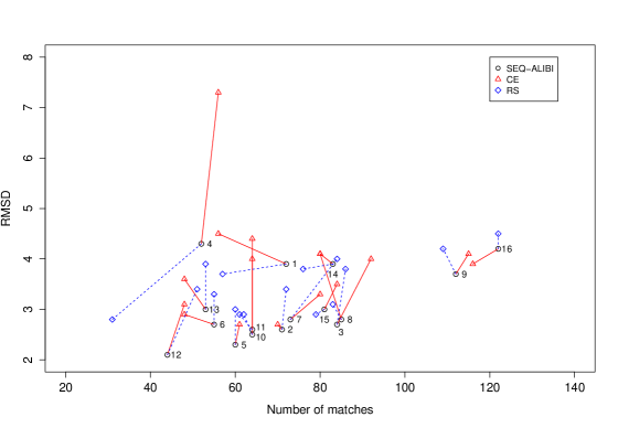
Figure 4: RMSD against number of matches for each of the $16$ protein pairs using SA, CE and RS. The pairs are numbered as in Table 2. For each pair, the line segments join the point for SA with the points for CE (solid line) and RS (dashed line).

4.4 Comparison $2$: MALIDUP data set

The MALIDUP (Manual ALIgnments of DUPlicated domains) (Cheng et al., , 2008) data set consists of $241$ protein pairs which can be used for a larger-scale comparison. Each pair has a corresponding reference alignment curated manually by experts.

We compare results from our method, SEQ-ALIBI (SA), with the manual alignments and those from DALI (Holm and Sander, , 1993), TMalign (TM) (Zhang and Skolnick, , 2005), DeepAlign (DA) (Wang et al., , 2013) and Matt (Menke et al., , 2008).

Figure 5: RMSDs (left) and alignment lengths (right) for SA, manual, DALI, TM, DA and Matt.

We see (Figure 5) that overall RMSD values are lower for SA than the other methods, except Matt, which is similar, but has shorter alignments generally (median 77 for SA and 74 for Matt). Overall, the distributions of alignment lengths are quite similar. As discussed in Section 1.2, it is difficult to use these quantities as absolute measures of performance, but the distributions give a sense of the general picture. Note that for the $3$ outlying RMSD values present in the other methods, SA matches fewer points than the other methods, and these extra points increase the RMSD dramatically.

Figure 6: GDT scores (left), TM scores (centre) and percentage of reference alignment matches found (right), for SA, manual, DALI, TM, DA and Matt on the MALIDUP data set.

The distributions of GDT and TM scores can be seen in Figure 6. For GDT scores, we see that the distribution for SA is similar to that of the manual alignments and Matt, and higher than DALI, TM and DA. For TMscore, SA gives higher scores overall than the other methods, apart from TM, which is not surprising since TM optimises TMscore.

For agreement with the manual reference alignments, SA performs similarly, perhaps slightly better, than TM and Matt (Figure 6). DALI and DeepAlign perform best overall. We observe that, for the pairs where SA has lower agreement with the reference alignment, the SA alignments tend to be longer and have lower RMSD than the manual alignment. Of course, the manual alignment is in some sense “correct”, since expert judgement is used to judge the most biologically-relevant alignment. SA is doing what it is expected to do, in that longer alignments with lower RMSD (after accounting for the gap penalty) will be preferred (the posterior density of such alignments will be higher). DeepAlign incorporates extra information, such as hydrogen bonding, which could explain the better agreement with the reference alignments. Our framework naturally allows for further information such as this to be incorporated.

4.5 Comparison $3$: RIPC data set

The RIPC data set (Mayr et al., , 2007) contains examples of particularly challenging test cases. The full data set consists of $40$ pairs of proteins, each of which exhibits one or more of the following challenging features: (R)epetitions, (I)ndels, (P)ermutations, (C)onformational changes. Due to the sequence order constraint of our prior on the alignment, it is not appropriate to consider permutations (which involve a reordering of subunits in a protein), which leaves $28$ pairs for our analysis.

For $13$ of the $28$ pairs, there are partial reference alignments, manually-curated, of amino acid residues which align, according to experts. They are not “complete” alignments, as they only indicate certain residues which match, which in some cases is only a few. Here, we compare SEQ-ALIBI, DeepAlign and Matt. Other methods which have performed well on the RIPC data set include DEDAL (Daniluk and Lesyng, , 2011), PROMATCH (Poleksic, , 2016), PAUL (Wohlers et al., , 2010) and MATRAS (Kawabata, , 2003).

The alignments from SEQ-ALIBI have lower RMSD overall (Figure 7). The distribution of alignment lengths is similar to that of DeepAlign, with Matt tending to give shorter alignments. SEQ-ALIBI tends to find alignments with higher GDT and TM scores (Figure 7).

Figure 7: RMSDs, alignment lengths, GDT scores and TM scores, respectively, for SEQ-ALIBI, DeepAlign and Matt on the RIPC data set.

Table 5: Percentage of the manually-aligned residues found by SEQ-ALIBI, DeepAlign and Matt for RIPC protein data. Also given are the types of challenge presented by each pair (C,I,R) and the number of aligned residues (matches) given in the reference alignment.

Pair	Challenge	Number of matches	% agreement	% agreement	% agreement
		in reference alignment	(SEQ-ALIBI)	(DeepAlign)	(Matt)
1	IC	4	75	75	75
2	I	10	100	90	100
3	I	3	33	100	100
4	I	3	33	100	100
5	IC	8	75	100	100
6	I	12	67	100	100
7	I	11	91	64	100
8	CR	148	43	49	0
9	CR	4	50	50	50
10	IC	4	100	100	100
11	C	101	50	72	85
12	C	220	58	70	95
13	IC	6	67	67	67

Results from the comparison to reference alignments are given in Table 5. SEQ-ALIBI does not perform quite as well as DeepAlign and Matt in terms of the percentage agreement with the reference alignment residues. We note that SEQ-ALIBI will prefer solutions with long alignments and lower RMSD, as such solutions will give higher posterior density. The better agreement of DeepAlign and Matt with the reference alignments could possibly be explained by the incorporation of amino acid type and hydrogen bonding information (DeepAlign) and allowing for protein flexibility (Matt). SEQ-ALIBI could be modified to include such information, and we would then expect to see more similarity in the alignments obtained. For example, amino acid type could be readily included by adding an additional factor into the likelihood which quantifies the quality of the primary structure alignment using BLOSUM or PAM matrices, as in Rodriguez and Schmidler, (2014). DeepAlign incorporates hydrogen bonding by looking at orientation of neighbouring residues and the location of the beta-carbon atoms of each residue. Our likelihood could be modified in a similar fashion to include this additional spatial information; see Mardia et al., (2007), who used beta-carbon information within the framework of the method of Green and Mardia, (2006) to refine alignments. Schmidler, (2010) has considered a Bayesian model for flexible shapes using changepoint ideas; with modifications to our model, similar ideas could be incorporated within our framework, to allow for protein flexibility as Matt does.

It should be noted that since some of the reference alignments involve small numbers of matches, the raw percentage of agreement can exaggerate any discrepancies. For example, for pair 3, there are only 3 reference matches, and the two missed by SEQ-ALIBI can be corrected by inserting a single gap. Hence, SEQ-ALIBI is only one index out from the reference alignment for both these matches. The gap inserted then allows 3 matches between amino acids of the same type, information which was used when curating the reference matches. Therefore, inclusion of amino acid type information in SEQ-ALIBI could balance against the penalty for inserting the required gap, and give alignments more similar to DeepAlign and Matt as suggested above. Similar observations apply to many of the other pairs, and there is less discrepancy between the three methods than it appears from looking at the raw percentage agreement with the reference matches.

4.6 Computational complexity

As MCMC is employed to sample from the joint posterior distribution, the running time is of course relatively slow when judged against the computational methods we compare with, which are specially designed to quickly find an optimal alignment and run in a matter of seconds. However, they are typically deterministic and return one optimum for a given set of input parameters, assuming the existence of a single global optimum. Multiple runs with different inputs would be needed to try and explore the space of potential alignments, with no clear principled way for doing this in general. Additionally, it is not clear that multiple “good” solutions corresponding to very different alignments (e.g. those requiring different spatial transformations) — different modes in probability terms — would be easily identified in this manner (Mayr et al., , 2007). Our simulation-based approach has the potential to explore multiple alignments in one run, and identify interesting competing alignments to be followed up, and hence complements these fast and efficient deterministic algorithms.

As an illustration, the example in Section 4.2 (configurations of $186$ and $226$ points) runs in around $90$ seconds for a single-chain run, and the parallel tempering implementation using $6$ chains in around $15$ minutes (run on a single core, 3.20GHz CPU). However, we have made no use of the potential for parallelisation, and our implementation is not necessarily the most efficient. As mentioned above, a major benefit of our approach is a framework which allows the space of alignments to be explored and quantified probabilistically in a fully coherent manner. MCMC is the standard approach for “exact” sampling-based inference based on complex probability distributions (i.e. that the target distribution is exactly the one of interest). There is potential for utilising approximations to the true target distribution, which would enable access to quick approximate solutions whilst retaining the fully probabilistic framework.

5 Discussion

In this paper we have presented a fully Bayesian model for the alignment of protein structures. The model is based on that of Green and Mardia, (2006), but accounts for the constraint that the sequence ordering of the points in each configuration is meaningful and must be preserved when matching pairs of points, which requires a different prior model for the matching matrix $\bm{M}$. Here we have concentrated on priors built from penalties which are functions of the sequence indices. We have illustrated the potential of this approach using a penalty function which allows the degree of proportionality in the indices defining the alignment to be controlled, which contains a commonly-used gap penalty function as a special case. The formulation allows for other penalty functions to be easily incorporated, and computation will be practical and efficient whenever MCMC updates change only a small number of terms which contribute to the overall penalty.

Rodriguez and Schmidler, (2014) have also developed a Bayesian model for protein structure alignment; we have used the same prior model for $\bm{M}$ as a starting point, but their method of sampling alignments from the posterior distribution is quite different to ours, in that an entire new alignment is sampled at each iteration as opposed to the small perturbations of our proposals. Additionally, the authors optimise over the registration parameters, which can be viewed as using a Laplace approximation to the marginal posterior distribution. We have treated the registration parameters as additional unknown parameters about which to draw inference, and sampling them from the posterior allows us to account for the extra uncertainty in the alignment as a result of the uncertainty in these parameters. We note that Kenobi and Dryden, (2012) have begun numerical comparisons between the two approaches in a particular situation, namely where rigid-body transformations are used and no sequence order constraint is imposed. The flexibility of the fully Bayesian method to handle different transformations and constraints has been further illustrated in this paper and the papers by Mardia et al., (2013) and Forbes et al., (2014). We have illustrated our method on challenging examples considered previously in the literature, and have shown our method to fare well on benchmark data sets alongside established computational methods, whilst offering more in terms of a fully probabilistic interpretation.

As we have focussed on alignments which preserve sequence order in this paper, our method is not appropriate for situations such as circular permutations of structural subunits (Mayr et al., , 2007). Such situations can be handled within our general framework, with appropriate modifications to the model/prior distribution. We note that additional information, such as amino acid types and hydrogen bonding (as in e.g. DeepAlign and Formatt) can be incorporated too. Our focus here has been to show how sequence order-constrained protein structure alignment can be modelled using Bayesian methods for unlabelled shape analysis, and such generalisations will be interesting avenues for further work. Though the running time is relatively slow (compared to highly-optimised computational algorithms) due to the use of MCMC (as is standard in Bayesian anlaysis of complex models), our approach offers something different in terms of a principled, fully-probabilistic framework giving access to a full posterior distribution over all possible alignments. In contrast, other methods are rather ad-hoc in nature, do not follow normative inferential principles, and/or deliver conclusions that either do not quantify the uncertainty in alignments, or the joint uncertainty in multiple matches. There is also scope for exploring fast approximations to the target posterior distribution. Our view is that probabilistic methods have their place alongside the more heuristic, but very efficient and successful, computational algorithms, and that both approaches can complement each other in any comprehensive analysis.

References

- Altschul, (1988) Altschul, S. F. (1988). Generalized affine gap costs for protein sequence alignment. Proteins: Structure, Function and Genetics, 32:88–96.
- Altschul et al., (1990) Altschul, S. F., Gish, W., Miller, W., Myers, E. W., and Lipman, D. J. (1990). Basic local alignment search tool. Journal of Molecular Biology, 215:403–410.
- Berman et al., (2000) Berman, H. M., Westbrook, J., Feng, Z., Gilliland, G., Bhat, T. N., Weissig, H., Shindyalov, I. N., and Bourne, N. E. (2000). The protein data bank. Nucleic Acids Research, 28:235–242.
- Boomsma et al., (2008) Boomsma, W., Mardia, K. V., Taylor, C. C., Ferkinghoff-Borg, J., Krogh, A., and Hamelryck, T. (2008). A generative, probabilistic model of local protein structure. Proc Natl Acad Sci U S A, 105(26):8932–7.
- Broderick et al., (2013) Broderick, T., Kulis, B., and Jordan, M. I. (2013). MAD-Bayes: MAP-based asymptotic derivations from Bayes. 30th International Conference on Machine Learning, 28.
- Cheng et al., (2008) Cheng, H., Kim, B., and Grishin, N. (2008). MALIDUP: a database of manually constructed structure alignments for duplicated domain pairs. Proteins: Structure, Function, and Bioinformatics, 70:1162–1166.
- (7) Daniels, N. M., Kumar, A., Cowen, L. J., and Menke, M. (2012a). Touring protein space with Matt. IEEE/ACM Trans. Comput. Biol. Bioinformatics, 9(1):286–293.
- (8) Daniels, N. M., Nadimpalli, S., and Cowen, L. J. (2012b). Formatt: Correcting protein multiple structural alignments by incorporating sequence alignment. BMC Bioinformatics, 13:259.
- Daniluk and Lesyng, (2011) Daniluk, P. and Lesyng, B. (2011). A novel method to compare protein structures using local descriptors. BMC Bioinformatics, 12:344.
- Dryden et al., (2007) Dryden, I. L., Hirst, J. D., and Melville, J. L. (2007). Statistical analysis of unlabeled point sets: comparing molecules in chemoinformatics. Biometrics, 63:237–251.
- Dryden and Mardia, (2016) Dryden, I. L. and Mardia, K. V. (2016). Statistical Shape Analysis, 2nd edn. Wiley, Chichester.
- Durbin et al., (1998) Durbin, R., Eddy, S., Krogh, A., and Mitchison, G. (1998). Biological Sequence Analysis: Probabilistic Models of Proteins and Nucleic Acids. Cambridge University Press, Cambridge.
- Forbes et al., (2014) Forbes, P. G. M., Lauritzen, S., and Moller, J. (2014). Fingerprint analysis with marked point processes. arXiv - 1407.5809.
- Gerstein and Levitt, (1998) Gerstein, M. and Levitt, M. (1998). Comprehensive assessment of automatic structural alignment against a manual standard, the scop classification of proteins. Protein Science, 7:445–456.
- Geyer, (1991) Geyer, C. J. (1991). Markov chain Monte Carlo maximum likelihood. In Computer Science and Statistics: Proc. 23rd Symp. Interface, pages 156–163.
- Gibrat et al., (1997) Gibrat, J., Madej, T., Spouge, J., and Bryant, S. (1997). The VAST protein structure compar-ison method. Biophysical Journal, 72:298.
- Godzik, (1996) Godzik, A. (1996). The structural alignment between two proteins: is there a unique answer? Protein Science, 1325–1338.
- Golden et al., (2017) Golden, M., Garcia-Portugues, E., Sorensen, M., Mardia, K. V., Hamelryck, T., and Hein, J. (2017). A generative angular model of protein structure evolution. Molecular Biology and Evolution, 34:2085–2100.
- Green, (2015) Green, P. J. (2015). MAD-Bayes matching and alignment for labelled and unlabelled configurations. In Dryden, I. L. and Kent, J. T., editors, Geometry Driven Statistics, pages 377–389. Wiley, Chichester.
- Green and Mardia, (2006) Green, P. J. and Mardia, K. V. (2006). Bayesian alignment using hierarchical models, with applications in protein bioinformatics. Biometrika, 93(2):235–254.
- Hasegawa and Holm, (2009) Hasegawa, H. and Holm, L. (2009). Advances and pitfalls of protein structural alignment. Current Opinion in Structural Biology, 19:341–348.
- Herman, (2019) Herman, J. L. (2019). Enhancing statistical multiple sequence alignment and tree inference using structural information. In Sikosek, T., editor, Computational Methods in Protein Evolution, pages 183–214. Springer New York, New York.
- Holm and Sander, (1993) Holm, L. and Sander, C. (1993). Protein structure comparison by alignment of distance matrices. Journal of Molecular Biology, 233:123–138.
- Jonker and Volgenant, (1987) Jonker, R. and Volgenant, A. (1987). A shortest augmenting path algorithm for dense and sparse linear assignment problems. Computing, 38:325–340.
- Jung and Lee, (2000) Jung, J. and Lee, B. (2000). Protein structure alignment using environmental profiles. Protein Engineering, 13:535–543.
- Kawabata, (2003) Kawabata, T. (2003). MATRAS: A program for 3D structure comparison. Nucleic Acids Research, 31:3367–3369.
- Kenobi and Dryden, (2012) Kenobi, K. and Dryden, I. L. (2012). Bayesian matching of unlabeled point sets using procrustes and configuration models. Bayesian Analysis, 7:547–566.
- Kent et al., (2010) Kent, J. T., Mardia, K. V., and Taylor, C. C. (2010). Matching unlabelled configurations and protein bioinformatics. Technical report, University of Leeds.
- Lennox et al., (2009) Lennox, K. P., Dahl, D. B., Vannucci, M., and Tsai, J. W. (2009). Density estimation for protein conformation angles using a bivariate von Mises distribution and Bayesian nonparametrics. Journal of the American Statistical Association, 104(486):586–596. PMID: 20221312.
- Liu and Lawrence, (1999) Liu, J. S. and Lawrence, C. E. (1999). Bayesian inference on biopolymer models. Bioinformatics, 15:38–52.
- Ma and Wang, (2014) Ma, J. and Wang, S. (2014). Algorithms, applications, and challenges of protein structure alignment. Advances in Protein Chemistry and Structural Biology, 94:121–175.
- Maadooliat et al., (2016) Maadooliat, M., Zhou, L., Najibi, S. M., Gao, X., and Huang, J. Z. (2016). Collective estimation of multiple bivariate density functions with application to angular-sampling-based protein loop modeling. Journal of the American Statistical Association, 111(513):43–56.
- Mardia, (2013) Mardia, K. V. (2013). Statistical approaches to three key challenges in protein structural bioinformatics. Journal of the Royal Statistical Society, Series C, 62:487–514.
- Mardia et al., (2013) Mardia, K. V., Fallaize, C. J., Barber, S., Jackson, R. M., and Theobald, D. L. (2013). Bayesian alignment of similarity shapes. The Annals of Applied Statistics, 7:989–1009.
- Mardia et al., (2007) Mardia, K. V., Nyirongo, V. B., Green, P. J., Gold, N. D., and Westhead, D. R. (2007). Bayesian refinement of protein functional site matching. BMC Bioinformatics, 8:257.
- Mayr et al., (2007) Mayr, G., Domingues, F. S., and Lackner, P. (2007). Comparative analysis of protein structure alignments. BMC Structural Biology, 7:50.
- Menke et al., (2008) Menke, M., Berger, B., and Cowen, L. (2008). Matt: Local flexibility aids protein multiple structure alignment. PLos Computational Biology, 4:e10.
- Myronenko and Song, (2010) Myronenko, A. and Song, X. (2010). Point set registration: coherent point drift. IEEE Transactions on Pattern Analysis and Machine Intelligence, 32:2262–2275.
- Najibi et al., (2017) Najibi, S. M., Maadooliat, M., Zhou, L., Huang, J. Z., and Gao, X. (2017). Protein structure classification and loop modeling using multiple Ramachandran distributions. Computational and Structural Biotechnology Journal, 15:243 – 254.
- Ortiz et al., (2002) Ortiz, A. R., Strauss, C. E. M., and Olmea, O. (2002). MAMMOTH (matching molecular models obtained from theory): An automated method for model comparison. Protein Science, 11:2606–2621.
- Poleksic, (2016) Poleksic, A. (2016). Detecting non-trivial protein structure relationships. Current Bioinformatics, 1(2):234–242.
- Rangarajan et al., (1997) Rangarajan, A., Chui, H., and Bookstein, F. L. (1997). The Softassign procrustes matching problem. In Information Processing in Medical Imaging, pages 29–42. Springer.
- Redelings and Suchard, (2005) Redelings, B. D. and Suchard, M. A. (2005). Joint Bayesian Estimation of Alignment and Phylogeny. Systematic Biology, 54(3):401–418.