A class of quintessential inflation models with parameter space consistent with BICEP2

Abstract

In this paper, we focus on general features of quintessential inflation which is an effort to unify inflation and dark energy using a single scalar field. We describe a class of models of quintessential inflation which can give rise to the tensor to scalar ratio of perturbations consistent with recent BICEP2 measurements. The scale of inflation in the model is around the GUT scale and there is large parameter space consistent with the recent findings.

I Introduction

One of the most outstanding and clean predictions of inflationary paradigm is related to relic gravity waves Grishchuk:1974ny ; Grishchuk:1977zz ; Starobinsky:1979ty ; Allen:1987bk ; Sahni:1990tx ; Souradeep:1992sm ; Giovannini:1998bp ; Giovannini:1999bh ; Langlois:2000ns ; Kobayashi:2003cn ; Hiramatsu:2003iz ; Easther:2003re ; Brustein:1995ah ; Gasperini:1992dp ; Giovannini:1999qj ; Giovannini:1997km ; Gasperini:1992pa ; Giovannini:2009kg ; Giovannini:2008zg ; Giovannini:2010yy ; Tashiro:2003qp ; Sahni:2001qp which are generated quantum mechanically in the early Universe. The primordial tensor perturbations induce B mode polarization in microwave background spectrum such that the effect depends upon the tensor to scalar ratio of perturbations $r$. Since the effect was not observed , the tensor to scalar ratio was supposed to be negligibly small. However, the recent observations on CMB polarization has demonstrated that the effect is sizeable, namely, the scalar to tensor ratio of perturbations, $r=0.2_{-0.05}^{+0.07}$ Ade:2014xna such that the scale of inflation is around the GUT scale.

Quintessential inflation Peebles:1999fz ; Sahni:2001qp ; Sami:2004xk ; Copeland:2000hn ; Huey:2001ae ; Majumdar:2001mm ; Dimopoulos:2000md ; Sami:2003my ; Dimopoulos:2002hm ; Rosenfeld:2005mt ; Giovannini:2003jw ; Dimopoulos:2002ug ; Nunes:2002wz ; Dimopoulos:2001qu ; Dimopoulos:2001ix ; Yahiro:2001uh ; Kaganovich:2000fc ; Peloso:1999dm ; Baccigalupi:1998mn ; Hossain:2014xha , a unified description of inflation and dark energy using a single scalar field, is necessarily followed by kinetic regime responsible for blue spectrum of relic gravity waves Giovannini:1998bp ; Giovannini:1999bh ; Giovannini:1999qj ; Sahni:2001qp . These scenarios can be classified into Type I and Type II. In first type, we consider models for which the scalar field potential is exponentially steep for most of the history of universe and only at late times the potential turns shallow. In Type II, we place models with potentials, shallow at early times followed by steep behavior thereafter. Ideally, quintessential inflation requires a potential that could felicitate slow roll in the early phase followed by approximately steep exponential behavior such that the potential turns shallow only at late times. Steep nature of potential is necessitated for the radiative regime to commence and peculiar steep behavior is needed to realize the scaling regime. However, the generic potentials do not change their character so frequently, they rather broadly come into two said categories:
Type A: The inverse power law and $\cos$ hyperbolic potentials belong to this category. In this case one requires to assist slow roll by an extra damping at early times. In Randall-Sundrum scenario Randall:1999ee ; Randall:1999vf , the high energy corrections to Einstein equations Shiromizu:1999wj give rise to brane-damping which assists slow roll along a steep potential Sahni:2001qp ; Copeland:2000hn ; Huey:2001ae ; Majumdar:2001mm ; Maartens:1999hf . As the field rolls down its potential, high energy corrections cease leading to graceful exit from inflation. Unfortunately, the tensor to scalar ratio in this case is too large, $r\simeq 0.4$ to be consistent with observations and the steep brane-world inflation is therefore ruled out.
Type B: In this case, the field potential stays steep after inflation. In this case, the late time behavior can be achieved by invoking an extra feature in the potential. For instance, massive neutrino matter with non-minimally coupled to scalar field can give rise to minimum of the potential at late times when neutrinos become non-relativistic Wetterich:2013jsa ; Hossain:2014xha .

In this paper, we shall describe a class of models of quintessential inflation of this category and look for parameter space which could comply with the recent measurement of B mode polarization spectrumAde:2014xna .

II The Model

The Einstein frame action of the desired model is given by Wetterich:2013jsa ; Hossain:2014xha ,

$$\mathcal{S}=\int d^{4}x\sqrt{-g}\bigg{[}-\frac{M_{\textrm{Pl}}^{2}}{2}R+\frac{k^{2}(\phi)}{2}\partial^{\mu}\phi\partial_{\mu}\phi+V(\phi)\bigg{]},~{}~{}~{}$$ (1)

$$k^{2}(\phi)=\left(\frac{\alpha^{2}-\tilde{\alpha}^{2}}{\tilde{\alpha}^{2}}\right)\frac{1}{1+\beta^{2}\mathrm{e}^{\alpha\phi/M_{\textrm{Pl}}}}+1\,,$$ (2)

where we assume the form of potential to be exponential, $V(\phi)=M_{\textrm{Pl}}^{4}\mathrm{e}^{-\alpha\phi/M_{\textrm{Pl}}}$; $\tilde{\alpha}$ controls slow roll such that $\tilde{\alpha}\gg 1$ and $\beta$ is associated with the scale of inflation Wetterich:2013jsa ; Hossain:2014xha . In the region of large $\phi$, the kinetic function $k(\phi)\to 1$ which reduces the action to scaling form provided $\alpha$ is large; nucleosynthesis constraint Ade:2013zuv implies that $\alpha\gtrsim 20$. One also checks that slow roll ensues for small field limit which continues in the region of large field (see, discussion below). Hence the kinetic function controls the inflationary and post inflationary behavior of the field. It is instructive to have cast the action in non canonical form.

Variation of action (1) with respect to the field $\phi$ gives its equation of motion, namely,

$$k^{2}\Box\phi+k\frac{\partial k}{\partial\phi}\partial^{\mu}\phi\partial_{\mu}\phi=\frac{\partial V}{\partial\phi}\,.$$ (3)

We can transform the scalar-field part of the action (1) to its canonical form through the transformation, $\sigma=\Bbbk(\phi)$ and $k(\phi)=\frac{\partial\Bbbk}{\partial\phi}$ Thus, (1) becomes

$$\mathcal{S}_{E} = \int d^{4}x\sqrt{g}\left[-\frac{M_{\textrm{Pl}}^{2}}{2}R+\frac{1}{2}\partial^{\mu}\sigma\partial_{\mu}\sigma+V(\Bbbk^{-1}(\sigma))\right].~{}~{}~{}\,$$ (4)

In case of small-field approximation, we have $k^{2}(\phi)\approx\alpha^{2}/\tilde{\alpha}^{2}$, $\sigma(\phi)\approx\frac{\alpha}{\tilde{\alpha}}\phi$ and the potential becomes $V_{\mathrm{s}}(\sigma)\approx M_{\textrm{Pl}}^{4}\mathrm{e}^{-\tilde{\alpha}\sigma/M_{\textrm{Pl}}}$ Hossain:2014xha which can give rise to slow roll for small values of $\tilde{\alpha}$. Similarly, for very large values of $\phi$, we have $k^{2}(\phi)\approx 1$ and

$$\sigma\approx\phi-\frac{2}{\tilde{\alpha}}\ln\left(\frac{\beta}{2}\right)+\frac{2}{\alpha}\ln\left(\frac{\tilde{\alpha}\beta}{\alpha+\tilde{\alpha}}\right)$$ (5)

and the potential reads $V_{l}(\sigma)\approx V_{l0}\mathrm{e}^{-\alpha\sigma/M_{\textrm{Pl}}}$ Hossain:2014xha , where $V_{l0}$ is expressed in terms of $M_{\textrm{Pl}}$, $\beta$ and $\tilde{\alpha}$.

III Inflation

The slow roll parameters can be easily expressed in terms of non-canonical field $\phi$ as

$$\epsilon = \frac{M_{\textrm{Pl}}^{2}}{2}\left(\frac{1}{V}\frac{{\rm d}V}{{\rm d}\sigma}\right)^{2}=\frac{M_{\textrm{Pl}}^{2}}{2k^{2}(\phi)}\left(\frac{1}{V}\frac{{\rm d}V}{{\rm d}\phi}\right)^{2}=\frac{\alpha^{2}}{2k^{2}(\phi)},~{}~{}\,\,$$ (6)

$$\eta = \frac{M_{\textrm{Pl}}^{2}}{V}\frac{{\rm d^{2}}V}{{\rm d}\sigma^{2}}=2\epsilon-\frac{M_{\textrm{Pl}}}{\alpha}\frac{{\rm d}\epsilon(\phi)}{{\rm d}\phi}\ ,$$ (7)

$$\xi^{2} = \frac{M_{\textrm{Pl}}^{4}}{V^{2}}\frac{{\rm d}V}{{\rm d}\sigma}\frac{{\rm d}^{3}V}{{\rm d}\sigma^{3}}=2\epsilon\eta-\frac{\alpha M_{\textrm{Pl}}}{k^{2}}\frac{{\rm d}\eta}{{\rm d}\phi}\,.$$ (8)

For $\alpha\gg 1$ and $\tilde{\alpha}\ll 1$, we can approximate the slow roll parameters as,

$$\epsilon=\frac{\tilde{\alpha}^{2}}{2}\left(1+X\right),~{}~{}\eta=\epsilon+\frac{\tilde{\alpha}^{2}}{2}~{}~{}{\text{and}}~{}~{}\xi^{2}=2\tilde{\alpha}^{2}\epsilon$$ (9)

where $X=\beta^{2}\mathrm{e}^{\alpha\phi/M_{\textrm{Pl}}}$. Power spectra of curvature and tensor perturbations are

$$\mathcal{P_{R}}(k) = A_{\mathrm{s}}(k/k_{*})^{n_{\mathrm{s}}-1+(1/2){\rm d}n_{\mathrm{s}}/{\rm d}\ln k\ln(k/k_{*})}\,,$$ (10)

$$\mathcal{P}_{\mathrm{t}}(k) = A_{\mathrm{t}}(k/k_{*})^{n_{\mathrm{t}}}\,,$$ (11)

where $A_{\mathrm{s}},\;A_{\mathrm{t}},\;n_{\mathrm{s}},\;n_{\mathrm{t}}\;{\rm and}\;{\rm d}n_{\mathrm{s}}/{\rm d}\ln k$ are scalar amplitude, tensor amplitude, scalar spectral index, tensor spectral index and its running respectively.

Number of e-foldings in the model is given by,

$$\mathcal{N}\approx\frac{1}{\tilde{\alpha}^{2}}\bigg{[}\ln\left(1+X^{-1}\right)-\ln\left(1+\frac{\tilde{\alpha}^{2}}{2}\right)\bigg{]}\,.$$ (12)

Considering $\tilde{\alpha}\ll 1$, we can approximate the above expression to

$$\mathcal{N}\approx\frac{1}{\tilde{\alpha}^{2}}\ln\left(1+X^{-1}\right)$$ (13)

which gives,

$$\epsilon(\mathcal{N})=\frac{\tilde{\alpha}^{2}}{2}\frac{1}{1-\mathrm{e}^{-\tilde{\alpha}^{2}\mathcal{N}}}\,.$$ (14)

For small field approximation that corresponds to the case $\tilde{\alpha}^{2}\gg 1/\mathcal{N}$, we notice that, ($X\ll 1$) $\epsilon=\eta/2=\tilde{\alpha}^{2}/2$. Whereas in large field limit ($X\gg 1$), we have $\epsilon=\eta/2=\tilde{\alpha}^{2}X/2$ in which case, $\tilde{\alpha}^{2}\ll 1/\mathcal{N}$. This means that the transition between the two regions happens when $\tilde{\alpha}^{2}\approx 1/\mathcal{N}$.

With the knowledge of $\epsilon(\mathcal{N},\tilde{\alpha})$ and $\eta(\mathcal{N},\tilde{\alpha})$, the tensor to scalar ratio ($r$), scalar spectral index ($n_{\mathrm{s}}$) and its running (${\rm d}n_{\mathrm{s}}/{\rm d}\ln k$) read as follows,

$$r(\mathcal{N},\tilde{\alpha}) \approx 16\epsilon(\mathcal{N})=\frac{8\tilde{\alpha}^{2}}{1-\mathrm{e}^{-\tilde{\alpha}^{2}\mathcal{N}}}\,,$$ (15)

$$n_{\mathrm{s}}(\mathcal{N},\tilde{\alpha}) \approx 1-6\epsilon+2\eta=1-\tilde{\alpha}^{2}\coth\left(\frac{\tilde{\alpha}^{2}\mathcal{N}}{2}\right)\,,$$ (16)

$$\frac{{\rm d}n_{\mathrm{s}}}{{\rm d}\ln k} \approx 16\epsilon\eta-24\epsilon^{2}-2\xi^{2}=-\frac{\tilde{\alpha}^{4}}{2\sinh^{2}\left(\frac{\tilde{\alpha}^{2}\mathcal{N}}{2}\right)}.~{}~{}~{}~{}$$ (17)

Figure 1: The tensor-to-scalar ratio ($r$) versus the model parameter $\tilde{\alpha}$, for different e-foldings $\mathcal{N}$. Blue (dashed), red (solid) and black (dotted) lines correspond to $\mathcal{N}=50$, $60$ and $70$ respectively. The shaded region marks the BICEP2 constraint on $r$ at $1\sigma$ confidence level, that is $r=0.2^{+0.07}_{-0.05}$ Ade:2014xna .

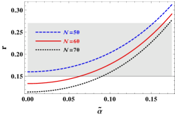
In Fig. 1 we present the variation of the tensor-to-scalar ratio ($r$) with respect to $\tilde{\alpha}$, for various numerical values of the number of e-foldings. Additionally, the shaded region marks the allowed values of $r$ in $1\sigma$ confidence level, given by BICEP2 Ade:2014xna collaboration. From BICEP2 results Ade:2014xna we have $r=0.2^{+0.07}_{-0.05}$ and Fig. 1 clearly shows that the values of $r$ allowed by the BICEP2 can be achieved in the model at hand by tuning the parameter $\tilde{\alpha}$, for instance $r\approx 0.2$ for $\tilde{\alpha}=0.12$ and $\mathcal{N}=60$. For these values of $\tilde{\alpha}$ and $\mathcal{N}$, using Eqs. (16) and (17), we find that $n_{\mathrm{s}}=0.965$ and ${\rm d}n_{\mathrm{s}}/{\rm d}\ln k=-0.000522$. While $n_{\mathrm{s}}$ satisfies the $1\sigma$ bound, $n_{\mathrm{s}}=0.9603\pm 0.0073$ from Planck results Ade:2013uln , the value of the running of $n_{\mathrm{s}}$ does not satisfy the $1\sigma$ bound ${\rm d}n_{\mathrm{s}}/{\rm d}\ln k=-0.021^{+0.012}_{-0.010}$ from the same collaboration.

Figure 2: 1$\sigma$ (blue) and 2$\sigma$ (cyan) contours for $Planck+WP+highL+BICEP2$ data, and 1$\sigma$ (red) and 2$\sigma$ (pink) contours for $Planck+WP+highL$ data, on the $n_{\mathrm{s}}-r$ plane. The black solid curves bound the region predicted in our model for efoldings between $\mathcal{N}=50$ and $\mathcal{N}=70$ and for the parameter $\tilde{\alpha}$ between $0^{+}$ and $0.175$. The lower line ($\tilde{\alpha}\to 0$) is for $\mathcal{N}$ from $50$ to 70, the left curve ($\mathcal{N}=50$) is for $\tilde{\alpha}$ from $0^{+}$ to 0.17, the right curve ($\mathcal{N}=70$) is for $\tilde{\alpha}$ from $0^{+}$ to 0.17, and the upper line ($\tilde{\alpha}=0.17$) is for $\mathcal{N}$ from $50$ to 70.

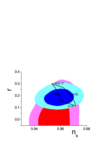
In Fig. 2, we present the $1\sigma$ (blue) and $2\sigma$ (cyan) likelihood contours on the $n_{\mathrm{s}}-r$ plane for the observations $Planck+WP+highL+BICEP2$ Ade:2014xna . For completeness, we additionally present the $1\sigma$ (red) and $2\sigma$ (pink) contours, from the data of $Planck+WP+highL$ Ade:2013uln . On top of these, we depict the predictions of the model at hand. In particular, the black solid curves bound the region predicted in our model for efoldings between $\mathcal{N}=50$ and $\mathcal{N}=70$ and for the parameter $\tilde{\alpha}$ between $0^{+}$ and $0.175$. This figure clearly shows that we can obtain a tensor-to-scalar ratio well within the $1\sigma$ (blue) confidence level by tuning the parameter $\tilde{\alpha}$. Furthermore, we have $r=-8n_{\mathrm{t}}$, which gives us the range of $n_{\mathrm{t}}$ as $-0.0338\leq n_{\mathrm{t}}\leq-0.0188$ for the given BICEP2 Ade:2014xna range of $r$ in $1\sigma$ confidence level.

The COBE normalized value of density perturbations is given by the following fitting function is Bunn:1996py ,

$$A_{\mathrm{s}}=1.91\times 10^{-5}\mathrm{e}^{1.01(1-n_{\mathrm{s}})}/\sqrt{1+.75r}\,.$$ (18)

BICEP2 Ade:2014xna gives the constraint on $r=0.2^{+0.07}_{-0.05}$ and Planck 2013 results Ade:2013uln gives $n_{\mathrm{s}}=0.9603\pm 0.0073$. So the COBE normalized value of density perturbations for the best fit values of $r$ and $n_{\mathrm{s}}$ taken from the BICEP2 Ade:2014xna and Planck Ade:2013uln observations respectively is $1.8539\times 10^{-5}$.

On the other hand, the scalar perturbation spectrum is given by

$$A^{2}_{\mathrm{s}}(k)=\frac{V}{\left(150\pi^{2}M_{\textrm{Pl}}^{4}\epsilon\right)}\,,$$ (19)

and at the horizon crossing ($k=k_{*}=a_{*}H_{*}$)

$$A^{2}_{\mathrm{s}}(k_{*})=7^{n_{s*}-1}\delta^{2}_{H}\,.$$ (20)

Moreover, the energy scale of inflation is given by

$$\!\!V_{*}^{1/4}=\left(\frac{7^{n_{s*}-1}r_{*}}{1-0.07r_{*}-0.512n_{s*}}\right)^{1/4}\!2.75\times 10^{16}~{}\rm GeV\,.$$ (21)

Since in the present model different values of $r$ and $n_{\mathrm{s}}$ can be obtained by changing the parameter $\tilde{\alpha}$ and efoldings $\mathcal{N}$ (see Fig. 1), we can use the above formulas in order to estimate the inflation scale. In particular, for the values of interest, $r=0.2$ and $n_{\mathrm{s}}=0.9603$, we get the energy scale of inflation to be $2.157\times 10^{16}\rm GeV$.

Using COBE normalization, we can also have a relation between the parameters $\tilde{\alpha}$, $\beta$ and e-foldings $\mathcal{N}$,

$$\frac{\beta^{2}\sinh^{2}\left(\tilde{\alpha}^{2}\mathcal{N}/2\right)}{\tilde{\alpha}^{2}}=6.36\times 10^{-8}\,,$$ (22)

which in case of large field approximation (that is for $\tilde{\alpha}^{2}\mathcal{N}\ll 1$ and $\beta^{2}\tilde{\alpha}^{2}=2.5\times 10^{-7}/\mathcal{N}^{2}$ for the given values) gives $r_{*}=0.2$ and $n_{s*}=0.9603$.

Let us note that the conventional (p)reheating mechanism does not work in quintessential inflation. However, instant preheating can be implemented in the scenario under consideration Hossain:2014xha . It is required that the field potential is steep in the post inflationary era, allowing radiative regime to commence. In this case, during scaling regime, $\Omega_{\phi}=4/\alpha^{2}$; nucleysynthesis from Planck results Ade:2013zuv then implies that $\alpha\gtrsim 20$ which in view of $\tilde{\alpha\ll 1}$ tells us that inflation ends at a sufficiently large value of $\phi$ or $X$. Indeed, the large-field slow-roll regime gives us $\epsilon=\eta=\tilde{\alpha}^{2}X/2\ \to\ X_{\rm end}=2/\tilde{\alpha}^{2}\gg 1$ and the kinetic function is given by $k^{2}(\phi)\simeq\alpha^{2}/(\tilde{\alpha}^{2}X)\ \to\ k_{\rm end}\simeq\alpha/\sqrt{2}$.

An important comment regarding the small and large field limit inflation is in order. As noticed before, the boundary of the two regions is given by $\tilde{\alpha}=\sqrt{1/\mathcal{N}}$. Thus, in case inflation commences in the large field regime, $\tilde{\alpha}$ needs to be small in order to collect the required number of e-foldings. However, if inflation begins around the boundary, the slow roll region is larger and we might improve upon the numerical values of $\tilde{\alpha}$ for the given number of e-foldings, thereby giving rise to larger values of $r$. In fact, the large field approximation does not lead to the desired result in view of the recent observations.

At the commencement of inflation we have

$$X_{\rm in}=\frac{1}{\left(\mathrm{e}^{\tilde{\alpha}^{2}\mathcal{N}}-1\right)}\,,$$ (23)

which gives us the value of the potential at the beginning of inflation

$$V_{\rm in}=M_{\textrm{Pl}}^{4}\beta^{2}\left(\mathrm{e}^{\tilde{\alpha}^{2}\mathcal{N}}-1\right)\,.$$ (24)

Now replacing $\beta$ from (22) we acquire

$$V_{\rm in}=\frac{2.5\times 10^{-7}\tilde{\alpha}^{2}M_{\textrm{Pl}}^{4}}{\left(1-\mathrm{e}^{-\tilde{\alpha}^{2}\mathcal{N}}\right)}\,.$$ (25)

$V_{\rm in}^{1/4}$ gives the scale of inflation as in relation (21) and for consistency check the value given by $V_{\rm in}$ should be same as that of (21). From Fig. 1 we can see that $r\approx 0.2$ for $\tilde{\alpha}\approx 0.12$ and $\mathcal{N}=60$, and for these values of $\alpha$ and $\mathcal{N}$ we obtain $V_{\rm in}^{1/4}=2.46\times 10^{16}\rm GeV$, which matches the value calculated from Eq. (21) for $r=0.2$ and $n_{\mathrm{s}}=0.9603$.

Finally, we also have

$$\frac{X_{\rm in}}{X_{\rm end}}=\frac{V_{\rm end}}{V_{\rm in}}=\frac{\tilde{\alpha}^{2}}{2\left(\mathrm{e}^{\tilde{\alpha}^{2}\mathcal{N}}-1\right)}\,,$$ (26)

which for large field limit reduces to $V_{\rm end}/V_{\rm in}=1/\left(2\mathcal{N}\right)$ Hossain:2014xha . During the inflationary phase of the universe the first Friedmann equation reduces to $3H^{2}M_{\textrm{Pl}}^{2}=V$, and this provides the ratio $H_{\rm end}/H_{\rm in}$. Therefore, at the end of inflation we have,

$$H_{\rm end}=\frac{M_{\textrm{Pl}}\beta\tilde{\alpha}}{\sqrt{6}}=\frac{1.02\times 10^{-4}\tilde{\alpha}^{2}M_{\textrm{Pl}}}{\sinh\left(\tilde{\alpha}^{2}\mathcal{N}/2\right)}\,.$$ (27)

IV Spectrum of relic gravity waves

One of the generic predictions of inflation includes the quantum mechanical production of relic gravity waves, whose spectral energy density depends upon the post inflationary equation-of-state parameter $\omega$ Sahni:1990tx ; Sahni:2001qp . The tensor perturbation is given by, $\delta\mathrm{g}_{ij}=a^{2}h_{ij}$ where $h_{ij}$ can be represented as $h_{ij}=h_{k}(\tau)\mathrm{e}^{-ikx}\mathrm{e}_{ij}$ ($\mathrm{e}_{ij}$ is the polarization tensor, $\tau$ is the conformal time defined as ${\rm d}\tau={\rm d}t/a$ and k is the comoving wave number defined as $k=2\pi a/\lambda$ where $\lambda$ being the wavelength) and satisfies the Klein-Gordon equation $\Box h_{ij}=0$ which reduces to,

$$\ddot{h}_{k}(\tau)+2\frac{\dot{a}}{a}\dot{h}_{k}(\tau)+k^{2}h_{k}(\tau)=0\,.$$ (28)

We will consider power-law expansion of the scale factor $a$ as $a\sim(t/t_{0})^{p}\sim(\tau/\tau_{0})^{(1-2\mu)/2}$ where $\mu=(1-3p)/2(1-p)$. For exponential inflation $\mu=3/2$ and the scale factor goes as $a\sim\tau_{0}/\tau$, where $|\tau|<|\tau_{0}|$. In order to compute the spectral energy density of gravity waves, we need to compute the Bogoliubov coefficients (for detailed calculations one can see Sahni:1990tx ; Sahni:2001qp ). In order to obtain the analytical expression one assumes inflation to be exponential. In that case, the spectral energy density $\tilde{\rho}_{\mathrm{g}}(k)$, after the transition from de Sitter to post inflationary phase, characterized by the equation-of-state parameter $\omega$, is given by Sahni:2001qp ,

$$\tilde{\rho}_{\mathrm{g}}(k)\propto k^{1-2|\mu|};~{}~{}\mu=\frac{3}{2}\left(\frac{\omega-1}{3\omega+1}\right).$$ (29)

In the model under consideration the post inflationary dynamics is described by the scalar field in the kinetic regime with $\omega_{\phi}=1$, which implies that $\rho_{\mathrm{g}}\propto k$ thereby a blue spectrum of gravity wave background. Let us again note that in our case as usual, $n_{\mathrm{t}}=-r/8$ is small which we ignored when assumed inflation to be exactly exponential. The blue spectrum in our proposal is solely attributed to the kinetic regime that follows quintessential inflation irrespective of the underlying model.

As demonstrated in Refs. Sahni:2001qp ; Giovannini:1998bp ; Giovannini:1999bh ; Giovannini:1999qj , the gravitational waves amplitude increases during the kinetic regime and this might come into conflict with nucleosynthesis at the commencement of radiative regime, in case the kinetic regime is long. Since the standard mechanism does not work here, One assumes that radiation with energy density $\rho_{\mathrm{r}}$ is produced via an alternative mechanism. The ratio of the field energy density to $\rho_{\mathrm{r}}$, can be compared with the ratio of the energy density in gravity waves $\rho_{\mathrm{g}}$ to radiation energy density at the beginning of radiative era, namely,

$$\left(\frac{\rho_{\phi}}{\rho_{\rm r}}\right)_{\rm end}=\frac{3\pi}{64h^{2}_{\rm GW}}\left(\frac{\rho_{\mathrm{g}}}{\rho_{\mathrm{r}}}\right)_{\rm eq},$$ (30)

where,

$$h^{2}_{\rm GW}=\frac{H_{\rm in}^{2}}{8\pi M_{\textrm{Pl}}^{2}}=\frac{3.315\times 10^{-9}\tilde{\alpha}^{2}}{1-\mathrm{e}^{-\tilde{\alpha}^{2}\mathcal{N}}}\,,$$ (31)

is the square of dimensionless gravity wave amplitude. Nucleosynthesis imposes a stringent constraint on the ratio of energy densities at equality, that is $\rho_{\mathrm{g}}/\rho_{\mathrm{r}}\lesssim 0.01$, thereby giving rise to the lower bound of $\rho_{\phi}/\rho_{\mathrm{r}}$ at the end of inflation which reads

$$\rho_{\mathrm{r},\rm end}\geq\frac{3.517\times 10^{-14}M_{\textrm{Pl}}^{4}\tilde{\alpha}^{6}\mathrm{e}^{\tilde{\alpha}^{2}\mathcal{N}/2}}{\sinh^{3}\left(\tilde{\alpha}^{2}\mathcal{N}/2\right)}\,,$$ (32)

and it also gives $T_{\rm end}=\rho^{1/4}_{r,\rm end}$. Now the bound on $r$ from BICEP2 Ade:2014xna gives the bound on $\tilde{\alpha}$ as $0.063\leq\tilde{\alpha}\leq 1.83$ for $\mathcal{N}=60$. For $\tilde{\alpha}=0.12$ and $\mathcal{N}=60$, $r\approx 0.2$ and we get the bound on the temperature at the end of inflation as, $T_{\rm end}\geq 6.65\times 10^{13}\rm GeV$. This condition cannot be met for instance if reheating is attempted via gravitational particle production, which is an inefficient mechanism.

It is possible to circumvent the problem of over-production of relic gravity waves if an efficient mechanism such as instant preheating Felder:1998vq ; Felder:1999pv ; Campos:2004nc is implemented Sahni:2001qp ; Hossain:2014xha .

The spectral energy density parameter of the relic gravitational wave is defined as,

$$\Omega_{\rm GW}(k)=\frac{\tilde{\rho}_{\mathrm{g}}(k)}{\rho_{\rm c}}\,,$$ (33)

where $\rho_{\rm c}$ is the critical energy density and (detailed calculations one can see Ref. Sahni:2001qp )

$$\Omega_{\rm GW}^{\rm(MD)}=\frac{3}{8\pi^{3}}h_{\rm GW}^{2}\Omega_{\mathrm{m}0}\left(\frac{\lambda}{\lambda_{\mathrm{h}}}\right)^{2}\,,\lambda_{\rm MD}<\lambda\leq\lambda_{\mathrm{h}},~{}~{}~{}~{}~{}~{}$$ (34)

$$\Omega_{\rm GW}^{\rm(RD)}(\lambda)=\frac{1}{6\pi}h_{\rm GW}^{2}\Omega_{\mathrm{r}0}\,,~{}~{}~{}~{}~{}~{}~{}~{}~{}\lambda_{\rm RD}<\lambda\leq\lambda_{\rm MD}\,,~{}~{}~{}~{}~{}$$ (35)

$$\Omega_{\rm GW}^{\rm(kin)}(\lambda)=\Omega_{\rm GW}^{\rm(RD)}\left(\frac{\lambda_{\rm RD}}{\lambda}\right)\,,~{}~{}~{}~{}~{}\lambda_{\rm kin}<\lambda\leq\lambda_{\rm RD}\,,~{}~{}~{}~{}~{}$$ (36)

where,

$$\lambda_{\mathrm{h}} = 2cH_{0}^{-1}\,,$$ (37)

$$\lambda_{\rm MD} = \frac{2\pi}{3}\lambda_{\mathrm{h}}\left(\frac{\Omega_{\mathrm{r}0}}{\Omega_{\mathrm{m}0}}\right)^{1/2}\,,$$ (38)

$$\lambda_{\rm RD} = 4\lambda_{\mathrm{h}}\left(\frac{\Omega_{\mathrm{m}0}}{\Omega_{\mathrm{r}0}}\right)^{1/2}\frac{T_{\rm MD}}{T_{\rm rh}}\,,$$ (39)

$$\lambda_{\rm kin} = cH_{\rm kin}^{-1}\left(\frac{T_{\rm rh}}{T_{0}}\right)\left(\frac{H_{\rm kin}}{H_{\rm rh}}\right)^{1/3}\,,$$ (40)

where matter, radiation and kinetic energy dominated epochs are represented by “MD”, “RD” and “kin” respectively. $H_{0}$, $\Omega_{\mathrm{m}0}$ and $\Omega_{\mathrm{r}0}$ are the present values of Hubble parameter, matter and radiation energy density parameters respectively. reheating temperature and Hubble parameter are represented by $T_{\rm rh}$ and $H_{\rm rh}$ respectively and we have taken reheating temperature and Hubble parameter approximately same as the temperature and Hubble parameter at the end of inflation.

Figure 3: The spectral energy density of the relic gravity wave background versus the wavelength $\lambda$. Blue (small dashed), red (long dashed) and cyan (dotted) lines correspond to reheating temperature $7\times 10^{13}\rm GeV$, $2.5\times 10^{14}\rm GeV$ and $8\times 10^{14}\rm GeV$ respectively. We have taken $\tilde{\alpha}=0.12$ and $\mathcal{N}=60$. Black solid lines represent the sensitivity curves of advanced LIGO and LISA.

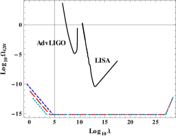
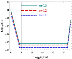
Fig. 3 shows the spectrum of the spectral energy density of relic gravitational waves with wavelength $\lambda$. Sensitivity curves of advanced LIGO aLIGO and LISA LISA1 are also depicted. Additionally, in Fig. 4 we present the spectrum of relic gravitational waves for different tensor to scalar ratio. We can write the amplitude of the relic gravitational wave ($h_{\rm GW}$) in terms of the tensor-to-scalar ratio ($r$) by using Eq. (15) and Eq. (31), and it is given as $h_{\rm GW}^{2}=3.315\times 10^{-9}r/8$. This implies that the square of the amplitude is directly proportional to $r$, and since the spectral energy density parameter of the relic gravitational wave ($\Omega_{\rm GW}$) is proportional to the square of the amplitude, $\Omega_{\rm GW}$ also gets increased with increasing $r$. This effect can be seen in Fig. 4.

Figure 4: The spectral energy density of the relic gravity wave background versus the wavelength $\lambda$. Blue (small dashed), red (long dashed) and cyan (solid) lines correspond to the tensor to scalar ratio $r=0.1,\;0.2\;{\rm and}\;0.3$ respectively with reheating temperature $10^{14}\rm GeV$. We have taken $\tilde{\alpha}=0.12$ and $\mathcal{N}=60$.

V Late time Evolution

Finally, let us point out for completeness that the late time acceleration, although not the subject here, can be achieved in the scenario by including massive neutrino matter, non-minimally coupled to the field Wetterich:2013jsa ; Hossain:2014xha . At late stage, when neutrinos become non relativistic, the field potential, originally a steep run-away potential, acquires a minimum allowing the exit from the scaling regime to dark energy Hossain:2014xha .

VI Conclusions

In this paper we have investigated a class of models that can successfully give rise to quintessential inflation. The Lagrangian of the single field system under consideration contains three free parameters $\tilde{\alpha}$, $\alpha$ and $\beta$ such that $\beta$ is related to scale of inflation and $\tilde{\alpha}$ defines the tensor to scalar ratio $r$ for a given number of efolds. As for $\alpha$, it is fixed by the post inflationary requirements, namely, nucleosynthesis constraint Ade:2013zuv .

For the observed values of $r$ from BICEP2 Ade:2014xna and $\mathcal{N}=60$, the parameter $\tilde{\alpha}$ in the model ranges from $0.063$ to $0.183$ consistent with the BICEP2 measurements, (see Fig. 1) such that the scale of inflation in this case is around the GUT scale. The distinguished feature of the model includes a blue spectrum of stochastic background of relic gravitational waves produced during inflation. The blue spectrum of relic gravity waves associated with the kinetic regime after inflation, is a generic feature of quintessential inflation irrespective of an underlying model Sahni:2001qp ; Sami:2004xk ; Giovannini:1998bp ; Giovannini:1999bh ; Giovannini:1999qj . However, the amplitude of relic gravity waves naturally depends upon the tensor to scalar ratio of perturbations and we have quoted here $\Omega_{\rm GW}$ in accordance with the observed values of $r$. Fig. 4 shows the $r$ dependence of spectral energy density parameter ($\Omega_{\rm GW}$). We should emphasize that we have neglected $n_{\mathrm{t}}$, the tilt of inflationary spectrum, in order to felicitate the analytical calculation. We reiterate that the blue spectrum here is nothing to do with blue tilt seen in BICEP2; the former is the consequence of kinetic regime which is a general feature in scenarios of quintessential inflation. We should also negligibly small values of running of the spectral index. note that the scenario under consideration predicts

The BICEP2 findings, if confirmed, would rule out a large number of models including the currently favourite Starobinsky model. In purely theoretical perspective, the GUT scale of inflation as envisaged by the said measurements would throw a big challenge to model building in the framework of effective field theories. We hope that the forthcoming announcement from Planck collaboration and future observations would clarify the related issues and the same is eagerly awaited.

VII Acknowledgments

We thank S.G. Ghosh, V. Sahni and T. Souradeep for useful discussions. MWH acknowledges CSIR, Govt. of India for financial support through SRF scheme. The research of ENS is implemented within the framework of the Action “Supporting Postdoctoral Researchers” of the Operational Program “Education and Lifelong Learning” (Actions Beneficiary: General Secretariat for Research and Technology), and is co-financed by the European Social Fund (ESF) and the Greek State.

References

- (1) L. P. Grishchuk, Sov. Phys. JETP 40, 409 (1975) [Zh. Eksp. Teor. Fiz. 67, 825 (1974)].
- (2) L. P. Grishchuk, Annals N. Y. Acad. Sci. 302, 439 (1977).
- (3) A. A. Starobinsky, JETP Lett. 30, 682 (1979) [Pisma Zh. Eksp. Teor. Fiz. 30, 719 (1979)].
- (4) B. Allen, Phys. Rev. D 37, 2078 (1988).
- (5) V. Sahni, Phys. Rev. D 42, 453 (1990).
- (6) T. Souradeep and V. Sahni, Mod. Phys. Lett. A 7, 3541 (1992) [hep-ph/9208217].
- (7) M. Giovannini, Phys. Rev. D 58, 083504 (1998) [hep- ph/9806329].
- (8) M. Giovannini, Phys. Rev. D 60, 123511 (1999) [as tro-ph/9903004].
- (9) D. Langlois, R. Maartens and D. Wands, Phys. Lett. B 489, 259 (2000) [hep-th/0006007].
- (10) V. Sahni, M. Sami and T. Souradeep, Phys. Rev. D 65, 023518 (2002) [gr-qc/0105121].
- (11) T. Kobayashi, H. Kudoh and T. Tanaka, Phys. Rev. D 68, 044025 (2003) [gr-qc/0305006].
- (12) T. Hiramatsu, K. Koyama and A. Taruya, Phys. Lett. B 578, 269 (2004) [hep-th/0308072].
- (13) R. Easther, D. Langlois, R. Maartens and D. Wands, JCAP 0310, 014 (2003) [hep-th/0308078].
- (14) R. Brustein, M. Gasperini, M. Giovannini and G. Veneziano, Phys. Lett. B 361, 45 (1995) [hep- th/9507017].
- (15) M. Gasperini and M. Giovannini, Phys. Rev. D 47, 1519 (1993) [gr-qc/9211021].
- (16) M. Giovannini, Class. Quant. Grav. 16, 2905 (1999) [hep- ph/9903263].
- (17) M. Giovannini, Phys. Rev. D 56, 3198 (1997) [hep- th/9706201].
- (18) M. Gasperini and M. Giovannini, Phys. Lett. B 282, 36 (1992).
- (19) M. Giovannini, PMC Phys. A 4, 1 (2010) [arXiv:0901.3026 [astro-ph.CO]].
- (20) M. Giovannini, Phys. Lett. B 668, 44 (2008) [arXiv:0807.1914 [astro-ph]].
- (21) M. Giovannini, Phys. Rev. D 81, 123003 (2010) [arXiv:1001.4172 [astro-ph.CO]].
- (22) H. Tashiro, T. Chiba and M. Sasaki, Class. Quant. Grav. 21, 1761 (2004) [gr-qc/0307068].
- (23) P. A. R. Ade et al. [BICEP2 Collaboration], arXiv:1403.3985 [astro-ph.CO].
- (24) P. J. E. Peebles and A. Vilenkin, Phys. Rev. D 60, 103506 (1999) [astro-ph/9904396].
- (25) M. Sami and V. Sahni, Phys. Rev. D 70, 083513 (2004) [hep-th/0402086].
- (26) E. J. Copeland, A. R. Liddle and J. E. Lidsey, Phys. Rev. D 64, 023509 (2001) [astro-ph/0006421].
- (27) G. Huey and J. E. Lidsey, Phys. Lett. B 514, 217 (2001) [astro-ph/0104006].
- (28) A. S. Majumdar, Phys. Rev. D 64, 083503 (2001) [as tro-ph/0105518].
- (29) K. Dimopoulos, Nucl. Phys. Proc. Suppl. 95, 70 (2001) [astro-ph/0012298].
- (30) M. Sami, N. Dadhich and T. Shiromizu, Phys. Lett. B 568, 118 (2003) [hep-th/0304187].
- (31) K. Dimopoulos, Phys. Rev. D 68, 123506 (2003) [as tro-ph/0212264].
- (32) R. Rosenfeld and J. A. Frieman, JCAP 0509, 003 (2005) [astro-ph/0504191].
- (33) M. Giovannini, Phys. Rev. D 67, 123512 (2003) [hep- ph/0301264].
- (34) K. Dimopoulos, astro-ph/0210374.
- (35) N. J. Nunes and E. J. Copeland, Phys. Rev. D 66, 043524 (2002) [astro-ph/0204115].
- (36) K. Dimopoulos, astro-ph/0111500.
- (37) K. Dimopoulos and J. W. F. Valle, Astropart. Phys. 18, 287 (2002) [astro-ph/0111417].
- (38) M. Yahiro, G. J. Mathews, K. Ichiki, T. Kajino and M. Orito, Phys. Rev. D 65, 063502 (2002) [as tro-ph/0106349].
- (39) A. B. Kaganovich, Phys. Rev. D 63, 025022 (2000) [hep- th/0007144].
- (40) M. Peloso and F. Rosati, JHEP 9912, 026 (1999) [hep- ph/9908271].
- (41) C. Baccigalupi and F. Perrotta, astro-ph/9811385.
- (42) M. W. Hossain, R. Myrzakulov, M. Sami and E. N. Saridakis, arXiv:1402.6661 [gr-qc].
- (43) L. Randall and R. Sundrum, Phys. Rev. Lett. 83, 4690 (1999) [hep-th/9906064].
- (44) L. Randall and R. Sundrum, Phys. Rev. Lett. 83, 3370 (1999) [hep-ph/9905221].
- (45) T. Shiromizu, K. -i. Maeda and M. Sasaki, Phys. Rev. D 62, 024012 (2000) [gr-qc/9910076].
- (46) R. Maartens, D. Wands, B. A. Bassett and I. Heard, Phys. Rev. D 62, 041301 (2000) [hep-ph/9912464].
- (47) C. Wetterich, Phys. Rev. D 89, 024005 (2014) [arXiv:1308.1019 [astro-ph.CO]].
- (48) P. A. R. Ade et al. [Planck Collaboration], arXiv:1303.5076 [astro-ph.CO].
- (49) P. A. R. Ade et al. [Planck Collaboration], [arXiv:1303.5082 [astro-ph.CO]].
- (50) E. F. Bunn, A. R. Liddle and M. J. White, 1, Phys. Rev. D 54, 5917 (1996) [astro-ph/9607038].
- (51) G. N. Felder, L. Kofman and A. D. Linde, Phys. Rev. D 59, 123523 (1999) [hep-ph/9812289].
- (52) G. N. Felder, L. Kofman and A. D. Linde, Phys. Rev. D 60, 103505 (1999) [hep-ph/9903350].
- (53) A. H. Campos, J. M. F. Maia and R. Rosenfeld, Phys. Rev. D 70, 023003 (2004) [astro-ph/0402413].
- (54) https://dcc.ligo.org/LIGO-T0900288/public
- (55) http://www.srl.caltech.edu/~shane/sensitivity/.