All-optical high-resolution magnetic resonance using a nitrogen-vacancy spin in diamond

Abstract

We propose an all-optical scheme to prolong the quantum coherence of a negatively charged nitrogen-vacancy (NV) center in diamond. Optical control of the NV spin suppresses energy fluctuations of the ${}^{3}\text{A}_{2}$ ground states and forms an energy gap protected subspace. By optical control, the spectral linewidth of magnetic resonance is much narrower and the measurement of the frequencies of magnetic field sources has higher resolution. The optical control also improves the sensitivity of the magnetic field detection and can provide measurement of the directions of signal sources.

I Introduction.

High-resolution magnetic resonance is currently one of the most important tools in many areas of science and technology, including analytical chemistry, materials science, structural biology, neuroscience, and medicine Ernst:1994:OxfordUniversityPress . However, the sensitivity of conventional techniques is restricted to large spin ensembles, which currently limits spatial resolution to the micrometer scale Ciobanu:2002:178 . Recently considerable attention has focused on the application of negatively charged nitrogen-vacancy (NV) centers in diamond as an atomic-sized magnetic field sensor to detect nuclear magnetic resonance (NMR) signals by quantum control with both laser fields and microwaves Degen:2008:243111 ; Maze:2008:644 ; Balasubramanian:2008:648 ; Zhao:2011:242 ; Zhao:2012:657 ; Mamin:2013:557 ; Staudacher:2013:561 ; London:2013:067601 ; Muller2013Draft ; Cai:2013:013020 . In these works, the NV centers are initialized and readout by optical fields Doherty:2013:1 ; Dobrovitski:2013:23 ; but the noise protection is based on pulsed Hahn:1950:580 ; Carr:1954:630 ; Naydenov:2011:081201 ; Yang:2010:2 ; Lidar:2013:QEC and continuous Cai:2012:113023 ; cai2012long dynamical decoupling techniques employing microwave control. Increasing the pulse rates in the case of pulsed dynamical decoupling and their Rabi frequencies in the case of continuous dynamical decoupling beyond the GHz regime is highly challenging. The requirement of realizing microwaves (which have wavelengths of centimeters) imposes limitations on the setup and individual microwave control on NV centers is difficult. Hence there has been a major effort to desirable to develop methods to overcome these shortcomings. All-optical control was recently shown to be possible Yale:2013:7595 , and an all-optical scheme for sensing the amplitudes of magnetic fields was demonstrated by electromagnetically induced transparency in an NV ensemble Acosta:2013:213605 . However to date, there are no all-optical methods to measure the frequencies of the magnetic fields which provides rich magnetic resonance information about the signal sources.

In this work, we propose an all-optical magnetic resonance scheme using a negatively charged NV center to measure the frequencies of magnetic fields [see Fig. 1(a)]. Unlike the magnetic resonance supported by dynamical decoupling, in our scheme fluctuations in optical control do not broaden the resonant signal peaks, and the frequency of magnetic resonance is determined by the energy gap of the ${}^{3}\text{A}_{2}$ ground sublevels, which can easily extend the sensing frequencies to the GHz range. The optical control of the NV center suppresses the energy fluctuations of the ${}^{3}\text{A}_{2}$ ground sublevels and significantly extends the coherence times of the NV centers. Since the magnetic resonance linewidth broadening by dephasing is eliminated through the optical control, high-resolution magnetic resonance with NV centers becomes possible. The all-optical magnetic resonance scheme may also have applications in solid-state GHz frequency standards and in all-optical quantum information processing with NV centers.

II A negatively charged NV center under optical control

In applications of negatively charged NV centers in quantum technologies, it is important to prolong the quantum coherence of the ${}^{3}\text{A}_{2}$ triplet spin ground states $|\pm 1_{g}\rangle=|E_{0}\rangle|\pm 1\rangle$ and $|0_{g}\rangle=|E_{0}\rangle|0\rangle$, where $|E_{0}\rangle$ refers to the orbital state with 0 orbital angular momentum projections along the NV axis. The relaxation time of an NV spin can approach 200 s at low temperatures (10 K) Jarmola:2012:197601 , whereas the dephasing time is relatively short, with typical values for the inhomogeneous dephasing time $T_{2}^{*}$ of 0.5 to 5 $\mu\text{s}$ Dobrovitski:2013:23 ; Doherty:2013:1 . With a large energy difference between $|0_{g}\rangle$ and $|\pm 1_{g}\rangle$, dephasing is the main source of decoherence and limits the overall decoherence time.

Figure 1: (color online). (a) NV level structure with optical control; a $\Lambda$ system is formed by the lasers resonantly driving the transitions between $|\pm 1_{g}\rangle$ and $|A_{2}\rangle$. (b) Energy diagram of a NV center in the dressed-state picture. The optical control induces a coherence protected space spanned by $|d_{g}\rangle$ and $|0_{g}\rangle$ (in yellow shadow), which is protected by the energy gaps $\pm\frac{\Omega}{2}$.

For simplicity, we model the dephasing by magnetic field fluctuations $\beta_{z}(t)$ on the NV axis (along $z$ direction), which couple to the NV spins through the Zeeman interaction ($\hbar=1$)

$$H_{\text{dep}}=\beta_{z}(t)S_{z},$$ (1)

with the spin operator $S_{z}=|+1_{g}\rangle\langle+1_{g}|-|-1_{g}\rangle\langle-1_{g}|$. We assume that $\beta_{z}(t)$ has zero-mean $\overline{\beta_{z}(t)}=0$, where the overline denotes ensemble averaging. The random field fluctuations $\beta_{z}(t)$ induce broadening of the states $|\pm 1_{g}\rangle$. An initial state of the center spin $|\Psi(0)\rangle=\sum_{k=\pm 1,0}a_{k}|k_{g}\rangle$ driven by $H_{\text{dep}}$ will evolve to $|\Psi(t)\rangle=a_{-1}e^{i\varphi(t)}|-1_{g}\rangle+a_{0}|0_{g}\rangle+a_{+1}e^{-i\varphi(t)}|+1_{g}\rangle$, where the accumulated random phase $\varphi(t)=\int_{0}^{t}\beta_{z}(\tau)d\tau$. The coherence between $|0_{g}\rangle$ and $|\pm 1_{g}\rangle$ is described by the average of the relative random phase factor $L_{0,\pm 1}=\overline{e^{\pm i\varphi(t)}}$, which vanishes when the random phase is large. For Gaussian noise, $L_{0,\pm 1}=\exp\left[-\frac{1}{2}\overline{\varphi(t)\varphi(t)}\right]$.

To suppress the dephasing using only optical control, we use two laser fields resonantly coupling the triplet ground states $|\pm 1_{g}\rangle$ to the ${}^{3}\text{E}$ excited state

$$|A_{2}\rangle=c_{+}|E_{-}\rangle|+1\rangle+c_{-}|E_{+}\rangle|-1\rangle,$$ (2)

with $|c_{+}|^{2}+|c_{-}|^{2}=1$ (see Fig. 1). The lasers also couple the states $|\pm 1_{g}\rangle$ and $|A_{1}\rangle=c_{-}^{*}|E_{-}\rangle|+1\rangle-c_{+}^{*}|E_{+}\rangle|-1\rangle$ but with a large detuning $\delta$, which is the energy gap between the states $|A_{2}\rangle$ and $|A_{1}\rangle$. The optical transitions between ${}^{3}\text{A}_{2}$ and ${}^{3}\text{E}$ are spin conserving Batalov:2009:195506 ; Togan:2010:730 ; Maze:2011:025025 . The state properties of the NV centers, such as the parameters $c_{+}$ and $c_{-}$, depend on electric, magnetic, and strain fields. The effective Hamiltonian to obtain the eigenstates and eigenenergies of the ${}^{3}\text{E}$ levels at low temperatures can be found in the review paper Doherty:2013:1 . To have well-resolved excited states, we put the NV center at cryogenic temperatures ($\lesssim 10$ K). Using $|E_{-}\rangle|+1\rangle=c_{+}^{*}|A_{2}\rangle+c_{-}|A_{1}\rangle$ and $|E_{+}\rangle|-1\rangle=c_{-}^{*}|A_{2}\rangle-c_{+}|A_{1}\rangle$, we have the Hamiltonian under constant optical control

$$H_{0} = \left(\Omega_{+}e^{i\phi_{+}}e^{i\omega_{+}t}\left[c_{+}^{*}|A_{2}\rangle+c_{-}|A_{1}\rangle\right]\langle+1_{g}|+\text{H. c.}\right)$$ (3)

$$+\left(\Omega_{-}e^{i\phi_{-}}e^{i\omega_{-}t}\left[c_{-}^{*}|A_{2}\rangle-c_{+}|A_{1}\rangle\right]\langle-1_{g}|+\text{H. c.}\right)$$

$$-\delta|A_{1}\rangle\langle A_{1}|+\sum_{k_{g}=\pm 1_{g},0_{g}}E_{k_{g}}|k_{g}\rangle\langle k_{g}|+H_{\text{dep}}+H_{\text{sig}},$$

where $\Omega_{\pm}$ are the Rabi frequencies and $E_{k_{g}}$ are the energies of the ground states. $\phi_{\pm}$ and $\omega_{\pm}$ are the phases and frequencies of the lasers, respectively. We also include an interaction Hamiltonian $H_{\text{sig}}$ for possible signal sources. The energy of $|A_{2}\rangle$ is set as the reference energy. The laser fields resonantly drive the transitions between $|\pm 1_{g}\rangle$ and $|A_{2}\rangle$ with the laser detuning $\Delta_{\pm 1_{g}}=E_{\pm 1_{g}}-\omega_{\pm}=0$. In the rotating frame of $e^{-iH_{g}t}$ with

$$H_{g}=\sum_{k_{g}=\pm 1_{g}}(E_{k_{g}}-\Delta_{k_{g}})|k_{g}\rangle\langle k_{g}|+E_{0_{g}}|0_{g}\rangle\langle 0_{g}|,$$ (4)

the system Hamiltonian reads

$$H=H_{L}+H_{\text{dep}}+\tilde{H}_{\text{sig}},$$ (5)

where

$$H_{L} = \left(\Omega_{+}e^{i\phi_{+}}\left[c_{+}^{*}|A_{2}\rangle+c_{-}|A_{1}\rangle\right]\langle+1_{g}|+\text{H. c.}\right)-\delta|A_{1}\rangle\langle A_{1}|$$ (6)

$$+\left(\Omega_{-}e^{i\phi_{-}}\left[c_{-}^{*}|A_{2}\rangle-c_{+}|A_{1}\rangle\right]\langle-1_{g}|+\text{H. c.}\right),$$

$$\tilde{H}_{\text{sig}}=e^{iH_{g}t}H_{\text{sig}}e^{-iH_{g}t}.$$ (7)

For accurate numerical simulations, we model the NV spin with 6 levels: three ground states $|\pm 1_{g}\rangle$ and $|0_{g}\rangle$, the two excited states $|A_{1}\rangle$ and $|A_{2}\rangle$, and a singlet state $|s\rangle$ to describe the intersystem crossing transitions. The dynamics of the NV center spin described by a density matrix $\rho(t)$ is governed by the Lindblad master equation Rivas:2012:OpenQuantumSystems ,

$$\frac{d}{dt}\rho=-i\left[H,\rho\right]+\sum_{\alpha,\beta}\gamma_{\beta\alpha}\left(\sigma_{\beta\alpha}\rho\sigma_{\alpha\beta}-\frac{1}{2}\rho\sigma_{\alpha\alpha}-\frac{1}{2}\sigma_{\alpha\alpha}\rho\right),$$ (8)

where the Lindblad operators $\sigma_{\beta\alpha}\equiv|\beta\rangle\langle\alpha|$, $\gamma_{\beta\alpha}$ are the decay rates, and the Hamiltonian $H$ is given by Eq. (5).

III Noise suppression by optical control

To illustrate the fundamental idea of noise suppression by optical control, we consider a simplified model without contributions from spontaneous decay (taken into account in detailed numerical simulations to present subsequently). When the energy gap $\delta\gg\Omega_{\pm}$, the coupling to $|A_{1}\rangle$ is negligible in Eq. (5), and we have the $\Lambda$-type Hamiltonian by dropping out terms related to the state $|A_{1}\rangle$,

$$H_{\Lambda}=H_{L2}+H_{\text{dep}}+\tilde{H}_{\text{sig}},$$ (9)

where

$$H_{L2}=\Omega|A_{2}\rangle\langle b_{g}|+\text{H. c.},$$ (10)

with the effective Rabi frequency

$$\Omega\equiv\sqrt{\Omega_{+}^{2}|c_{+}|^{2}+\Omega_{-}^{2}|c_{-}|^{2}},$$ (11)

and the bright state

$$|b_{g}\rangle\equiv\frac{1}{\Omega}\left(c_{+}\Omega_{+}e^{-i\phi_{+}}|+1_{g}\rangle+c_{-}\Omega_{-}e^{-i\phi_{-}}|-1_{g}\rangle\right).$$ (12)

The laser driving fields form a $\Lambda$ system with an excited state $|A_{2}\rangle$ and two ground states $|\pm 1_{g}\rangle$ (see Fig. 1). The dark state decoupled from the laser is

$$|d_{g}\rangle\equiv e^{i\varphi_{d}}\frac{1}{\Omega}\left(c_{-}^{*}\Omega_{-}e^{-i\phi_{+}}|+1_{g}\rangle-c_{+}^{*}\Omega_{+}e^{-i\phi_{-}}|-1_{g}\rangle\right),$$ (13)

with a global phase $\varphi_{d}=\text{Arc}(c_{+}c_{-})$. The laser Hamiltonian $H_{L2}$ has the eigenstates $|d_{g}\rangle$, $|0_{g}\rangle$, and $|l_{\pm}\rangle=\frac{1}{\sqrt{2}}\left(|b_{g}\rangle\pm|A_{2}\rangle\right)$ with energies $E_{l\pm}=\pm\frac{\Omega}{2}$. The subspace spanned by the two states $|d_{g}\rangle$ and $|0_{g}\rangle$ are separated from the other eigenstates $|l_{\pm}\rangle$ by the energy gaps $\pm\frac{\Omega}{2}$. Therefore the transitions from this subspace to $|l_{\pm}\rangle$ are suppressed by an energy penalty that is proportional to the Rabi frequency of the optical driving fields (see Fig. 1 and Ref. Timoney:2011:185 ).

The spin operator $S_{z}$ in the basis of $|b_{g}\rangle$ and $|d_{g}\rangle$ reads

$$S_{z} = \frac{1}{\Omega}\left(2e^{-i\varphi_{d}}c_{+}\Omega_{+}c_{-}\Omega_{-}\right)|d_{g}\rangle\langle b_{g}|+\text{H.c.}$$ (14)

$$+\kappa\left(|b_{g}\rangle\langle b_{g}|-|d_{g}\rangle\langle d_{g}|\right).$$

where $\kappa=\frac{1}{\Omega}\left(|c_{+}\Omega_{+}|^{2}-|c_{-}\Omega_{-}|^{2}\right)\leq 1$. To suppress the dephasing of the NV spin using the energy penalty $\frac{\Omega}{2}$, we choose the laser fields that satisfy

$$|c_{+}\Omega_{+}|=|c_{-}\Omega_{-}|.$$ (15)

Under such a condition, the spin operator $S_{z}$ becomes

$$S_{z}=|b_{g}\rangle\langle d_{g}|+\text{H.c.}=\frac{1}{\sqrt{2}}\left(|l_{+}\rangle+|l_{-}\rangle\right)\langle d_{g}|+\text{H.c.},$$ (16)

with

$$|b_{g}\rangle=e^{i\varphi_{b}}\frac{1}{\sqrt{2}}\left[|+1_{g}\rangle+e^{i\phi_{L}}|-1_{g}\rangle\right],$$ (17)

$$|d_{g}\rangle=e^{i\varphi_{b}}\frac{1}{\sqrt{2}}\left[|+1_{g}\rangle-e^{i\phi_{L}}|-1_{g}\rangle\right].$$ (18)

where $\varphi_{b}=\text{Arc}(c_{+}\Omega_{+}e^{-i\phi_{+}})$ and $\phi_{L}=\text{Arc}(\Omega_{+}\Omega_{-}c_{+}^{*}c_{-})+\phi_{+}-\phi_{-}$ is a tunable relative phase. With a relative large $\Omega$, the spectral power density of the magnetic field fluctuations $\beta_{z}(t)$ at the frequencies around the energy gap $\frac{\Omega}{2}$ is negligible. The off-resonant fluctuations $\beta_{z}(t)$ cannot induce the transitions from $|d_{g}\rangle$ to $|l_{\pm}\rangle$, which are strongly suppressed by the energy penalty $\pm\frac{\Omega}{2}$ [see Fig. 1(b)]. Because fluctuations in the effective Rabi frequency $\Omega$ only cause small changes in the magnitudes of the energy gap, our scheme is stable against the fluctuations of $\Omega$ Timoney:2011:185 , as long as the magnitudes of the energy gap are still much larger than the fluctuation frequencies of $\beta_{z}(t)$. When there are relative fluctuations in $\Omega_{\pm}$ and $c_{\pm}$, the second line in Eq. (14) does not vanish, and a fraction $\sim\kappa$ of the noise will not be suppressed by the energy gaps $\pm\frac{\Omega}{2}$ made by the optical control. The decoherence time caused by this fraction of noise is estimated to be $T_{\text{frac}}\sim T_{2}^{*}/\kappa$, and the fluctuations only cause negligible effects if $T_{\text{frac}}$ is much larger than the controlled evolution time. The relative amplitude fluctuations in the driving fields can be made very small if the fields are obtained from the same laser.

To manifest the effects of dephasing, we set $\tilde{H}_{\text{sig}}=0$ in Eq. (9). The quantum coherence between, e.g., $|0_{g}\rangle$ and $|d_{g}\rangle$ is described by the average

$$L_{0,d_{g}}(t)=\overline{\langle d_{g}|U_{\Lambda}(t)|d_{g}\rangle\langle 0_{g}|U_{\Lambda}^{\dagger}(t)|0_{g}\rangle},$$ (19)

where $U_{\Lambda}(t)=\mathcal{T}e^{-i\int_{0}^{t}H_{\Lambda}d\tau}$ with the time-ordering operator $\mathcal{T}$. The coherence $L_{0,d_{g}}(t)$ can be simplified as

$$L_{0,d_{g}}(t) = \overline{\langle d_{g}|\tilde{U}_{\text{dep}}(t)|d_{g}\rangle},$$ (20)

by using the transformation $\tilde{U}_{\text{dep}}(t)\equiv e^{iH_{L2}t}U_{\Lambda}(t)=\mathcal{T}e^{-i\int_{0}^{t}\tilde{H}_{\text{dep}}(\tau)d\tau}$ with

$$\tilde{H}_{\text{dep}}(t) =e^{iH_{L2}t}H_{\text{dep}}e^{-iH_{L2}t}$$ (21)

$$=\beta_{z}(t)\left(\cos\frac{\Omega t}{2}|b_{g}\rangle-i\sin\frac{\Omega t}{2}|A_{2}\rangle\right)\langle d_{g}|+\text{H.c.}.$$ (22)

The coherence between $|0_{g}\rangle$ and $|d_{g}\rangle$ decreases when the absolute value of $L_{0,d_{g}}(t)$ decreases. Without optical driving fields, $L_{0,d_{g}}(t)=\exp\left[-\frac{1}{2}\overline{\left(\int_{0}^{t}\beta_{z}d\tau\right)^{2}}\right]$ for Gaussian noise and vanishes when the random phase is large. From the expression of Eq. (22), we can see that when the noise is relatively slow compared to the frequency $\frac{\Omega}{2}$, the effect of the noise $\beta_{z}(t)$ is averaged out by the oscillating functions $\cos\frac{\Omega t}{2}$ and $\sin\frac{\Omega t}{2}$. Dynamical decoupling also uses similar modulation functions to average out unwanted noise Yang:2010:2 ; Lidar:2013:QEC ; Cai:2012:113023 ; cai2012long . A more detailed analysis in frequency domain is given in Appendix A.

Figure 2: (color online). Quantum coherence between states $|d_{g}\rangle$ and $|0_{g}\rangle$ at the moment $t=50\leavevmode\nobreak\ \mu$s as a function $\Omega$, for (a) $B_{z,\text{bias}}=0$ and (b ) $B_{z,\text{bias}}\approx 0.1$ T. The data were obtained by $4\times 10^{4}$ runs of averaging.

To demonstrate our scheme, we performed numerical simulations by implementing the master equation (8), including the spontaneous decay and dephasing. We used the parameters in the experimental paper Yale:2013:7595 for the numerical simulation. The decay rate from the excited states $|A_{1}\rangle$ and $|A_{2}\rangle$ to the ground sates $|\pm 1_{g}\rangle$ and $|0_{g}\rangle$ is $\gamma_{g,e}\approx 17$ MHz; the rate for intersystem crossing from the excited states to the singlet $|s\rangle$ is $\gamma_{s,e}\approx 37$ MHz; the inverse intersystem crossing rate from $|s\rangle$ to the ground states is $\gamma_{g,s}\approx 2.7$ MHz. In the simulation, the noise fluctuations $\beta_{z}(t)$ were simulated by the Ornstein-Uhlenbeck process Wang:1945:323 , which is Gaussian. Generated by the Ornstein-Uhlenbeck processes, the expectation value of $\beta_{z}(t)$ is $\overline{\beta_{z}(t)}_{\text{OU}}=\beta_{z}(t_{0})e^{-(t-t_{0})/\tau_{\beta}}$; the two-point correlation $\overline{\beta_{z}(t)\beta_{z}(t^{\prime})}_{\text{OU}}=\frac{c_{\beta}\tau_{\beta}}{2}e^{-|t-t^{\prime}|\tau_{\beta}}(1-e^{-2(t-t_{0})/\tau_{\beta}})$, where $t_{0}$ is the starting time to generate an Ornstein-Uhlenbeck process and $c_{\beta}$ is a diffusion coefficient Bibbona:2008:S117 . These quantities converge to stationary values after a time larger than the correlation time $\tau_{\beta}$. In the simulation, we chose $\beta_{z}(t_{0})=0$ for $\overline{\beta_{z}(t)}=0$. We used $t_{0}=-10\tau_{\beta}$ and simulated the spin dynamic at $t\geq 0$, so that $e^{-2(t-t_{0})/\tau_{\beta}}\approx 0$ and we had an exponentially-decaying correlation function $\overline{\beta_{z}(t)\beta_{z}(t^{\prime})}\approx\frac{c_{\beta}\tau_{\beta}}{2}e^{-|t-t^{\prime}|\tau_{\beta}}$. At $t\geq 0$, $\beta_{z}(t)$ can be treated as stationary stochastic process. We chose the correlation time $\tau_{\beta}=25$ $\mu\text{s}$ in the simulation de2010universal . The realizations of Ornstein-Uhlenbeck processes were generated by the exact simulation algorithm in Ref. Gillespie:1996:2084 ,

$$\beta(t+\Delta t)=\beta(t)e^{-\Delta t/\tau_{\beta}}+n_{\text{G}}\sqrt{\frac{c_{\beta}\tau_{\beta}}{2}(1-e^{-2\Delta t/\tau_{\beta}})},$$ (23)

which requires the generation of a unit Gaussian random number $n_{\text{G}}$ at each time step. The algorithm is exact because the update algorithm Eq. (23) is valid for any finite time step $\Delta t$ Gillespie:1996:2084 . We chose the value of the diffusion coefficient $c_{\beta}\approx 4/(T_{2}^{*2}\tau_{\beta})$ so that without optical driving fields $L_{0,\pm 1}(T_{2}^{*})=e^{-1}$ at the dephasing time $T_{2}^{*}=3$ $\mu\text{s}$.

To demonstrate the coherence protection by optical control, we prepared the quantum state in the superposition $|\Psi(0)\rangle=\frac{1}{\sqrt{2}}\left(|d_{g}\rangle+|0_{g}\rangle\right)$ of $|d_{g}\rangle$ and $|0_{g}\rangle$. To obtain the optimal amplitude of driving fields, we plotted the coherence $|L_{0,d_{g}}(t)|$ at $t=50$ $\mu$s at different $\Omega$ in Fig. 2. By increasing the driving amplitude $\Omega$, the quantum coherence was recovered by suppressing the noise effects. However, increasing $\Omega$ also increases the coupling to the state $|A_{1}\rangle$ [see Eq. (6)], which degrades the approximated $\Lambda$-type system [see Eq. (9)] and leads to population leakage out of the subspace spanned by $|d_{g}\rangle$ and $|0_{g}\rangle$. At zero static field, the energy gap $\delta\approx 2$ GHz and the mixing coefficients $|c_{+}|=|c_{-}|$ in Eq. (6), and therefore $|d_{g}\rangle$ only directly couples to $|A_{1}\rangle$. For $\Omega\ll\delta$, the population to $|A_{1}\rangle$ state is $\sim\left({\Omega}/{\delta}\right)^{2}$, estimated by time-independent perturbation theory. The value of $L_{0,d_{g}}(t)$ at a moment $t$ decreases when the leakage $\sim\left({\Omega}/{\delta}\right)^{2}\gamma_{e}t$ increases. Here $\gamma_{e}$ is the estimated decay rate from the excited states. In Fig. 2(a), the optimal control with $\Omega\sim 10$ MHz gives the best coherence protection. We can increase $\delta$ by applying a static bias magnetic field $B_{z,\text{bias}}$ along the axis of the NV center (z direction). However, non-zero $B_{z,\text{bias}}$ also changes the mixing coefficients $c_{\pm}$. For example, $B_{z,\text{bias}}=0.1$ T gives $\delta\approx 5.71$ GHz, $c_{+}\approx 0.984$, and $c_{-}\approx 0.178$. When $|c_{+}|\neq|c_{-}|$, the dark state $|d\rangle$ can transit to both excited states $|A_{1}\rangle$ and $|A_{2}\rangle$, and $|L_{0,d_{g}}(t)|$ is strongly reduced [see Fig. 2(b)]. At $B_{z,\text{bias}}=0.1$ T, the effective Rabi frequency $\Omega\sim 7$ MHz yields the best coherence protection.

In Fig. 3, we plot the quantum coherence as a function of time for cases of free induction decay ($\Omega=0$) and with optical driving fields ($\Omega=10$ MHz) at zero static fields. With an optical Rabi frequency $\Omega=10$ MHz, the coherence is significantly prolonged and exceeds 50 $\mu$s, which is over 16-fold improvement in the coherence time $T_{2}^{*}\approx 3$ $\mu$s.

Figure 3: (color online). Coherence between states $|d_{g}\rangle$ and $|0_{g}\rangle$ for cases without optical control ($\Omega=0$, blue dots) and with optical control ($\Omega=10$ MHz, red squares) at $B_{z,\text{bias}}=0$. The data were obtained by $4\times 10^{4}$ runs of averaging.

Although the scheme is robust to the fluctuations of $\Omega$ Timoney:2011:185 , Eq. (15) shows that independent fluctuations $\delta\Omega_{\pm}(t)$ in the amplitudes of $\Omega_{\pm}$ change the bright and dark states in Eqs. (17) and (18). To demonstrate that the scheme is not sensitive to independent fluctuations $\delta\Omega_{\pm}(t)$, we modelled $\delta\Omega_{\pm}(t)$ by Ornstein-Uhlenbeck processes. We selected a diffusion coefficient $c_{\Omega}=2\delta_{\Omega}^{2}/\tau_{\Omega}$ with a correlation time $\tau_{\Omega}=100$ $\mu$s and a variance of relative fluctuations $\overline{[\delta\Omega_{\pm}(t)/\Omega_{\pm}]^{2}}=\delta_{\Omega}^{2}$. The impact of independent intensity fluctuations on the coherence is shown in Fig. 4. The scheme still provides good performance even though the standard deviation of relative fluctuations $\delta_{\Omega}$ reaches $\sim 0.02$.

Figure 4: (color online). Coherence between the states $|d_{g}\rangle$ and $|0_{g}\rangle$ as a function of the standard deviation of relative fluctuation $\delta_{\Omega}$, at the moment $t=50\leavevmode\nobreak\ \mu$s. (a) $B_{z,\text{bias}}=0$ and $\Omega=10$ MHz; (b) $B_{z,\text{bias}}\approx 0.1$ T and $\Omega=7$ MHz. The data were obtained by $4\times 10^{4}$ runs of averaging.

IV High-resolution magnetic resonance by optical control

In magnetic resonance spectroscopy, when the energy gap, e.g., $\epsilon_{0,-1}\equiv E_{0}-E_{-1}$ between $|0_{g}\rangle$ and $|-1_{g}\rangle$, coincides with the frequency of the magnetic field, resonance transitions induce a signal peak in the frequency domain. The linewidth and depth of the peak determine the resolution and sensitivity of the spectroscopy. Because of the energy broadening induced by the random fluctuations $\beta_{z}(t)$, the minimum linewidth of the signal peak is limited by the deviation of the fluctuations $\sim\left(\overline{\beta_{z}(t)^{2}}\right)^{1/2}$. When the dephasing (i.e., the effect of energy broadening) is suppressed, we achieve a narrower linewidth, and hence spectroscopy with higher accuracy.

We assume that the signal fields have negligible frequency components around the energy gap $\frac{\Omega}{2}$. The signal Hamiltonian in Eq. (9) is written as

$$\tilde{H}_{\text{sig}}=\eta_{\text{sig}}(t)e^{iH_{g}t}\left[S_{x}\cos\theta_{\text{sig}}+S_{y}\sin\theta_{\text{sig}}\right]e^{-iH_{g}t},$$ (24)

where $\eta_{\text{sig}}(t)$ is the magnetic signal field with zero mean $\overline{\eta_{\text{sig}}(t)}=0$ and $\theta_{\text{sig}}$ is the direction of the magnetic field in the $x-y$ plane normal to the NV axis. We initialize the NV center in the state $|0_{g}\rangle$ by optical pumping. The population that remains in the initial state $|0_{g}\rangle$ is approximately governed by the dynamics induced by $H_{\Lambda}$ given by Eq. (9),

$$P_{|0_{g}\rangle}(t)=\overline{|\langle 0_{g}|e^{-i\int_{0}^{t}H_{\Lambda}d\tau}|0_{g}\rangle|^{2}}.$$ (25)

In the simulation, we generated single-frequency sources $\eta_{\text{sig}}(t)=\eta_{0}\cos(\omega_{s}t+\varphi_{s})$ with initial random phases $\varphi_{s}$ at each run of the simulation. To have the accurate resonance frequency $\omega_{\text{Res}}$, we diagonalized the Hamiltonian $H$ given by Eq. (6), as $\omega_{\text{Res}}$ is the energy between $|0_{g}\rangle$ and the state $|\tilde{d}_{g}\rangle$ which is approximately $|d_{g}\rangle$ and has a little mixing with the excited states $|A_{2}\rangle$ and $|A_{1}\rangle$. For $\Omega\ll\delta$, $\omega_{\text{Res}}\approx\epsilon_{0,-1}$, up to a correction $\sim\Omega^{2}/\delta$. We consider the magnetic resonance signal where the difference between the signal frequency and the resonant frequency is small, i.e., $|\omega_{s}-\omega_{\text{Res}}|\ll\omega_{\text{Res}}$. This enables the application of a rotating wave approximation by neglecting oscillating terms with frequencies $\sim 2\omega_{\text{Res}}$ in Eq. (24). The simulations used the master equation (8) with the Hamiltonian Eq. (5).

IV.1 Measurement of signal frequencies

Figure 5: (color online). Magnetic resonance signals for the NV center in zero field ($B_{z,\text{bias}}=0$) at the moment $t=50\leavevmode\nobreak\ \mu$s, for the cases without optical control (blue dots) and with optical control ($\Omega=10$ MHz, red squares). The amplitude of the magnetic source fields $\eta_{0}=0.01$ MHz. The green triangles are the resonance signal for the case where $\Omega_{\pm}$ have independent fluctuations with a relative standard deviation $\delta_{\Omega}=0.005$. The data were obtained by $10^{4}$ runs of averaging.

When there is no static bias field $(B_{z,\text{bias}}=0)$, $\delta\approx 2\leavevmode\nobreak\ \text{GHz}$, the states $|\pm 1_{g}\rangle$ are degenerate, and

$$\tilde{H}_{\text{sig}}=\eta_{\text{sig}}(t)e^{-i\epsilon_{0,-1}t}e^{-i\theta_{\text{sig}}}\frac{1}{\sqrt{2}}\left(|+1_{g}\rangle+|-1_{g}\rangle e^{i2\theta_{\text{sig}}}\right)\langle 0_{g}|+\text{H.c.}.$$ (26)

By choosing the laser phase $\phi_{L}=2\theta_{\text{sig}}+\pi$, we achieve the largest sensitivity as the signal Hamiltonian $\tilde{H}_{\text{sig}}=\eta_{\text{sig}}(t)e^{-i\epsilon_{01}t}e^{-i\theta_{\text{sig}}}e^{-i\varphi_{b}}|d_{g}\rangle\langle 0_{g}|+\text{H.c.}.$ The states $|d_{g}\rangle$ and $|0_{g}\rangle$ are coherence protected. We obtain the magnetic resonance signal by tuning the resonant frequency. When the resonant frequency is tuned to the frequency of the signal fields, the state $|0_{g}\rangle$ will transit to $|d_{g}\rangle$ and the change of $P_{|0_{g}\rangle}(t)$ gives the signal.

In Fig. 5, we plot the magnetic resonance signal at the evolution time $t=50$ $\mu$s. The laser phase is $\phi_{L}=2\theta_{\text{sig}}+\pi$, and the signal fields have an amplitude $\eta_{0}=0.01$ MHz. Without optical control, the signal fields with frequency $\omega_{\text{Res}}$ lead to a maximum resonant population change $\Delta P_{|0_{g}\rangle}\approx 21\%$ with a linewidth $\Delta\omega_{\text{FWHM}}\approx 0.2$ MHz (defined by the full width at half maximum); while with optical control $\Omega=10$ MHz, the signal induces a much larger population dip $\Delta P_{|0_{g}\rangle}\approx 63\%$ with a much narrower linewidth $\Delta\omega_{\text{FWHM}}\approx 0.02$ MHz, which is limited by the evolution time $t$ (within the coherence time range).

To reduce the resonance frequency $\omega_{\text{Res}}$ within the MHz range, we apply a static bias magnetic field along the axis of the NV center to narrow the energy gap $\epsilon_{0,-1}$. When the magnetic field $B_{z,\text{bias}}\approx 0.1$ T, $\delta\approx 5.7\leavevmode\nobreak\ \text{GHz}$, the ground states $|0_{g}\rangle$ and $|-1_{g}\rangle$ have an energy gap within the MHz range, and the energy gap between $|0_{g}\rangle$ and $|1_{g}\rangle$ is large ($\gtrsim 2.9$ GHz). For large energy gaps between $|0_{g}\rangle$ and $|1_{g}\rangle$, the transition from $|0_{g}\rangle$ to $|1_{g}\rangle$ induced by signal fields is negligible and we have

$$\tilde{H}_{\text{sig}}\approx\eta_{\text{sig}}(t)\frac{1}{2}e^{-i\epsilon_{0,-1}t}e^{i(\theta_{\text{sig}}-\varphi_{b}-\phi_{L})}\left(|b_{g}\rangle-|d_{g}\rangle\right)\langle 0_{g}|+\text{H.c.}.$$ (27)

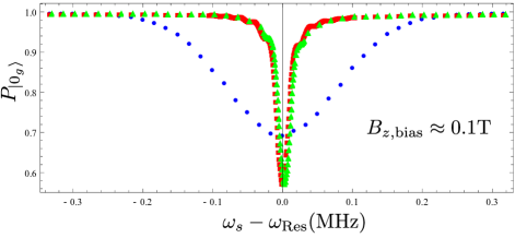
Figure 6: (color online). Magnetic resonance signals for the NV center in a bias field $B_{z,\text{bias}}\approx 0.1$ T at the moment $t=50\leavevmode\nobreak\ \mu$s, for the cases without optical control (blue dots) and with optical control $\Omega=7$ MHz (red squares). The amplitude of the magnetic source fields $\eta_{0}=0.02$ MHz. The green triangles are the resonance signal for the case where $\Omega_{\pm}$ have independent fluctuations with a relative standard deviation $\delta_{\Omega}=0.005$. The data were obtained by $10^{4}$ runs of averaging.

Under optical control with a large $\Omega$, we can ensure that the spectral density of $\beta_{z}(t)$ around $\frac{\Omega}{2}$ and $\eta_{\text{sig}}(t)$ around $\epsilon_{0,-1}\pm\frac{\Omega}{2}$ is negligible. The transitions between $|0_{g}\rangle$ and $|b_{g}\rangle$ are suppressed, and we get

$$\tilde{H}_{\text{sig}}\approx-\eta_{\text{sig}}(t)\frac{1}{2}e^{-i\epsilon_{0,-1}t}e^{i(\theta_{\text{sig}}-\varphi_{b}-\phi_{L})}|d_{g}\rangle\langle 0_{g}|+\text{H.c.}.$$ (28)

Therefore, when the field $\eta_{\text{sig}}(t)$ is on resonant with the transition frequency around $\omega_{\text{Res}}\approx\epsilon_{0,-1}$, the population of $|0_{g}\rangle$ decreases. In this way, the Fourier components of the signal source $\eta_{\text{sig}}(t)$ can be measured in high resolution. In Fig. 6, $\eta_{0}=0.02$ MHz, $B_{z,\text{bias}}\approx 0.1$ T, and the evolution time $t=50$ $\mu$s. Without optical control, the signal fields lead to a maximum population dip $\Delta P_{|0_{g}\rangle}\approx 30\%$ with a linewidth $\Delta\omega_{\text{FWHM}}\approx 0.2$ MHz; while with optical control $\Omega=7$ MHz, the population has a larger peak $\Delta P_{|0_{g}\rangle}\approx 42\%$ with a much narrower linewidth $\Delta\omega_{\text{FWHM}}\approx 0.02$ MHz limited by finite evolution time.

In Figs. 5 and 6, we also plot the magnetic resonance signals for optical control with independent driving fluctuations $\delta\Omega_{\pm}(t)$. It can be seen that an experimentally reachable standard deviation of relative fluctuations $\delta_{\Omega}=0.005$ only induces tiny changes in the magnetic resonance signal.

IV.2 Measurement of the directions of signal sources

For the case of $(B_{z,\text{bias}}=0)$, the signal Hamiltonian Eq. (26) depends on the direction $\theta_{\text{sig}}$ of the signal source. Note that the transition from $|0_{g}\rangle$ to $|b_{g}\rangle$ is suppressed when there is optical control. If $\phi_{L}=2\theta_{\text{sig}}$ in Eq. (26), the effect of the signal Hamiltonian $\tilde{H}_{\text{sig}}=\eta_{\text{sig}}(t)e^{-i\epsilon_{01}t}e^{-i\theta_{\text{sig}}}e^{-i\varphi_{b}}|b_{g}\rangle\langle 0_{g}|+\text{H.c.}$ is suppressed by the energy gap between $|0_{g}\rangle$ and $|b_{g}\rangle$ states, and the population change $\Delta P_{|0_{g}\rangle}$ is small. We have shown that the signal is large when the laser phase $\phi_{L}=2\theta_{\text{sig}}+\pi$. We use this phase dependence to determine the direction $\theta_{\text{sig}}$ of the signal field.

In Fig. 7, we applied a resonant signal field at the frequency $\omega_{s}=\omega_{\text{Res}}$ and tuned the laser phase $\phi_{L}=2\theta+\pi$ with different angles $\theta$. The control strength $\Omega=10$ MHz and the amplitude of the signal field $\eta_{0}=0.01$ MHz. From the lowest point in Fig. 7, we can infer the direction $\theta_{\text{sig}}$ of the signal source in the $x-y$ plane. For the case without optical control, $x$ and $y$ directions are equivilent and it is obvious that we cannot infer the direction of the signal source in the $x-y$ plane. Note that if the laser phase $\phi_{L}$ has a small deviation in the region $2(\theta_{\text{sig}}-0.1\pi)+\pi\lesssim\phi_{L}\lesssim 2(\theta_{\text{sig}}+0.1\pi)+\pi$, the signal $\Delta P_{|0_{g}\rangle}$ is also large with little change $(\approx 1\%)$. Therefore, our scheme is robust to fluctuations of laser phase.

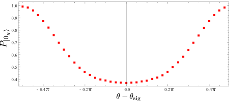
Figure 7: (color online). The on-resonant ($\omega_{s}=\omega_{\text{Res}}$) magnetic signal (the change of the population in $|0_{g}\rangle$) as a function of the angle difference $\theta-\theta_{\text{sig}}$ at the moment $t=50\leavevmode\nobreak\ \mu$s. The parameters $B_{z,\text{bias}}\approx 0$, $\Omega=10$ MHz, and $\eta_{0}=0.01$ MHz. The data were obtained by $5\times 10^{3}$ runs of averaging.

IV.3 Sensitivity enhanced by optical control

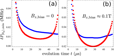
Figure 8: (color online). The one-trial sensitivity of the magnetic resonance signal at the resonant frequency $\omega_{s}=\omega_{\text{Res}}$ for the cases of without optical control (blue dots) and with optical control (red squares). (a) $B_{z,\text{bias}}=0$, $\eta_{0}=0.01$ MHz, and $\Omega=10$ MHz; (b) $B_{z,\text{bias}}\approx 0.1$ T, $\eta_{0}=0.02$ MHz, and $\Omega=7$ MHz. The data were obtained by $10^{5}$ runs of averaging.

Note that in Figs. 5 and 6, the signal peaks with optical control are more pronounced. This implies that the sensitivity is also improved when the dephasing noise is suppressed by the optical control. In Fig. 8, we plot the one-trial sensitivity $\delta P_{|0_{g}\rangle,\text{min}}=\Delta P_{|0_{g}\rangle}/(\frac{\partial P_{|0_{g}\rangle}}{\partial\eta_{0}})$ for the cases of the bias magnetic field $B_{z,\text{bias}}\approx 0$ and $B_{z,\text{bias}}\approx 0.1$ T, respectively. The parameters are the same as those for the optical sensing in Figs. 5 and 6 with $\omega_{s}=\omega_{\text{Res}}$. Here $\Delta P_{|0_{g}\rangle}=\sqrt{P_{|0_{g}\rangle}(1-P_{|0_{g}\rangle})}$ is the standard deviation of the population $P_{|0_{g}\rangle}$ in one measurement. Averaging the data by repeating the measurement $N$ times improves the sensitivity by a factor of $\alpha_{s}=1/\sqrt{N}$. If we perform the experiment for a given time $T_{\text{all}}$, we have $N=T_{\text{all}}/(T_{\text{init}}+t)$, where $T_{\text{init}}$ is the time for both initialization and readout and $t$ is the evolution time of the NV spin. With a large bias field, the transition from $|0_{g}\rangle$ to $|+1_{g}\rangle$ is suppressed by the energy gap between $|0_{g}\rangle$ and $|+1_{g}\rangle$ [see Eq. (27)]. Therefore the effective signal strength is reduced and the sensitivity with optical control is reduced in Fig. 6 at a short sensing time $t\lesssim 10$ $\mu$s. At a longer sensing time, the benefits from decohernce suppression by optical control manifest and the sensitivity is improved. At zero bias field, the transition from $|0_{g}\rangle$ to $|+1_{g}\rangle$ is kept under optical control, and the one-trial sensitivity is improved for a wide range of times $t\lesssim 45$ $\mu$s in the figure. The reduction of the one-trial sensitivity with optical control at $t\gtrsim 45$ $\mu$s is caused by the leakage of the population out of the $\Lambda$-type system.

V Discussion and conclusion

We have proposed an all-optical scheme to prolong the quantum coherence of a negatively charged NV center in diamond. With the quantum coherence extended and the energy fluctuations in the ${}^{3}\text{A}_{2}$ ground sublevels suppressed by the optical driving fields, we have achieved magnetic resonance with much narrower spectral linewidth and higher detection sensitivity. Unlike magnetic resonance by pulse sequences or more generally by dynamical decoupling, in our scheme driving field fluctuations do not broaden the resonant signal peaks. The sensing frequency by optical control is determined by the energy gap of the NV ${}^{3}\text{A}_{2}$ ground sublevels, which can easily reach the GHz range and enables stable GHz frequency standards in solids. At zero field, the magnetic resonance spectrum also enables measurement of the direction of signal sources in the plane perpendicular to the NV symmetry axis. The performance of the all-optical scheme has been confirmed by numerical simulations, by selecting the driving amplitudes within a range where the transitions to the off-resonant excited state are small and the $\Lambda$-type optical transition is a good approximation. Although we apply the optical driving fields on NV centers in diamond, the method is general and is applicable to other systems where a $\Lambda$-type optical transition can be formed.

Appendix A Decoherence function in the frequency domain

Here we outline the decoherence suppression by optical control in the frequency domain. For simplicity, we consider a simplified model without contributions from spontaneous decay and examine the effect of $\beta_{z}(t)$ up to the second order:

$$L_{0,d_{g}}(t)=1-\frac{1}{2}\int_{0}^{t}dt_{1}\int_{0}^{t_{1}}dt_{2}\overline{\beta_{z}(t_{1})\beta_{z}(t_{2})}M(t_{1},t_{2}),$$ (29)

where the modulation function

$$M(t_{1},t_{2}) = \cos\frac{\Omega t_{1}}{2}\cos\frac{\Omega t_{2}}{2}+\sin\frac{\Omega t_{1}}{2}\sin\frac{\Omega t_{2}}{2},$$ (30)

$$= \cos\left[\frac{\Omega}{2}(t_{1}-t_{2})\right].$$ (31)

With $M(t_{1},t_{2})=M(t_{2},t_{1})$ and the symmetry $\overline{\beta_{z}(t_{1})\beta_{z}(t_{2})}=\overline{\beta_{z}(t_{2})\beta_{z}(t_{1})}$ for classical noise, we have

$$L_{0,d_{g}}(t)=1-\frac{1}{2}\int_{0}^{t}dt_{1}\int_{0}^{t}dt_{2}\overline{\beta_{z}(t_{1})\beta_{z}(t_{2})}M(t_{1},t_{2}).$$ (32)

We assume stationary noise; i.e., noise with time translation symmetry, $\overline{\beta_{z}(t_{2})\beta_{z}(t_{1})}=\overline{\beta_{z}(t_{2}-t_{1})\beta_{z}(0)}$. We write

$$L_{0,d_{g}}(t)=1-\frac{1}{2}\int_{-\infty}^{\infty}\frac{d\omega}{2\pi}S_{\beta}(\omega)\tilde{M}(\omega),$$ (33)

in terms of the spectral power density

$$S_{\beta}(\omega)=\int_{-\infty}^{\infty}dt\overline{\beta_{z}(t)\beta_{z}(0)}e^{i\omega t},$$ (34)

and the filter function

$$\tilde{M}(\omega)=\int_{0}^{t}dt_{1}\int_{0}^{t}dt_{2}e^{-i\omega(t_{1}-t_{2})}M(t_{1},t_{2}).$$ (35)

Without optical control, i.e., $\Omega=0$, the function $\tilde{M}(\omega)=4\sin^{2}\left(\frac{\omega t}{2}\right)/\omega^{2}$ cannot filter out low-frequency fluctuations, which are dominant sources of decoherence. With large optical driving fields, the filter function $\tilde{M}(\omega)\approx C_{\omega,\Omega}\sin^{2}\left(\frac{\Delta_{\omega,\Omega}t}{2}\right)/\Delta_{\omega,\Omega}^{2}$ with $C_{\omega,\Omega}=4\omega\Omega/(\omega+\frac{\Omega}{2})^{2}$ has a power-law decay with the deviation $\Delta_{\omega,\Omega}=|\omega-\frac{\Omega}{2}|$, and the low frequency fluctuations are filtered out for large $\Omega$. In this simplified model, when the spectral power density around the frequency $\frac{\Omega}{2}$ is negligible, $|L_{0,d_{g}}(t)|\approx 1$ and the decoherence is strongly suppressed.