Long time simulation of a highly oscillatory Vlasov equation with an exponential integrator

Abstract

We change a previous time-stepping algorithm for solving a multi-scale Vlasov-Poisson system within a Particle-In-Cell method, in order to do accurate long time simulations. As an exponential integrator, the new scheme allows to use large time steps compared to the size of oscillations in the solution.

1 Introduction

In this paper, we improve the time numerical scheme introduced in [3], in order to make long time simulation of the following Vlasov equation

$$\left\{\begin{aligned} &\frac{\partial f_{\varepsilon}}{\partial t}+\frac{v}{\varepsilon}\frac{\partial f_{\varepsilon}}{\partial r}+\Big{(}-\frac{r}{\varepsilon}+E_{\varepsilon}(r,t)\Big{)}\frac{\partial f_{\varepsilon}}{\partial v}=0,\\ &f_{\varepsilon}\negthickspace\left(0,r,v\right)=f_{0}\left(r,v\right),\end{aligned}\right.$$ (1.1)

where $0<\varepsilon\ll 1$, $r\in\mathbb{R}$ is the position variable, $v\in\mathbb{R}$ the velocity variable, $f_{\varepsilon}=f_{\varepsilon}(r,v,t)$ is the distribution function, $f_{0}$ is given, and $-\frac{r}{\varepsilon}+E_{\varepsilon}(r,t)$ corresponds to the electric field. The difficulty in the numerical solution of this equation lies mainly in the multi-scale aspect due to the small parameter $\varepsilon$.

The main application will be the case when the electric field $E_{\varepsilon}$ is obtained by solving the Poisson equation. We will thus have to solve the following nonlinear system of equations

$$\left\{\begin{aligned} &\frac{\partial f_{\varepsilon}}{\partial t}+\frac{v}{\varepsilon}\frac{\partial f_{\varepsilon}}{\partial r}+\big{(}-\frac{r}{\varepsilon}+E_{\varepsilon}\left(r,t\right)\big{)}\frac{\partial f_{\varepsilon}}{\partial v}=0,\\ &\frac{\partial}{\partial r}\big{(}rE_{\varepsilon}\big{)}=\rho_{\varepsilon}\negmedspace\left(t,r\right),\hskip 8.53581pt\rho_{\varepsilon}\negmedspace\left(t,r\right)=\int_{\mathbb{R}}f_{\varepsilon}\left(t,r,v\right)dv,\\ &f_{\varepsilon}\negthickspace\left(0,r,v\right)=f_{0}\left(r,v\right).\end{aligned}\right.$$ (1.2)

This simplified model of the full Vlasov-Maxwell system is particularly adapted to the study of long and thin beams of charged particles within the paraxial approximation assuming that the beam is axisymmetric (see [4] and the references therein).

We will also test our scheme when

$$E_{\varepsilon}(r,t)=-r^{3}.$$ (1.3)

As in [3], we solve numerically the Vlasov equation by a particle method, which consists in approximating the distribution function by a finite number of macroparticles (see [1]). The trajectories of these particles are computed from the characteristic curves of the Vlasov equation, whereas the term $E_{\varepsilon}$ is computed, when obtained from the Poisson equation, on a mesh in the physical space. The contribution of this work is to improve the time numerical scheme proposed in [3], for solving in long times the stiff characteristics associated to equation (1.1)

$$\left\{\begin{aligned} &\frac{\text{d}R}{\text{d}t}=\frac{V}{\varepsilon},\\ &\frac{\text{d}V}{\text{d}t}=-\frac{R}{\varepsilon}+E_{\varepsilon}(R,t),\end{aligned}\right.$$ (1.4)

provided with the initial conditions $R(0)=r$, $V(0)=v$. We note that when $E_{\varepsilon}$ is given by (1.3), solving (1.4) reduces to solve the undamped and undriven Duffing equation

$$R^{\prime\prime}\left(t\right)+\frac{R(t)}{\varepsilon^{2}}+\frac{R^{3}(t)}{\varepsilon}=0$$ (1.5)

with initial conditions $R(0)=r$, $R^{\prime}(0)=v/\varepsilon$.

The solution of (1.1) is represented by a beam of particles in phase space moving along the characteristics curves (1.4). When the electric field $E_{\varepsilon}$ is zero the beam rotate around the origin with period $2\pi\varepsilon$. Otherwise, the dynamical system (1.4) can be viewed as a perturbation of the system obtained when the electric field is zero (see [7]). When the electric field $E_{\varepsilon}$ is obtained by solving the Poisson equation or if it is given by (1.3), the beam evolves by rotating around the origin in the phase space, and in long times a bunch forms around the center of the beam from which filaments of particles are going out. Classical explicit numerical methods require very small time step in order to capture the fast rotation. Consequently, long time simulations are very tedious.

In [3] the authors introduced a new explicit scheme based on Exponential Time Differencing (ETD) integrators (see [2] and [6]). The idea of the algorithm was the following: first, for each macroparticle as initial condition, we solve the ODE in (1.4) over some fast (i.e. of order $\varepsilon$) time by using a 4th order Runge-Kutta solver. The fast time is the same for all the macroparticles. Then, by means of the variation-of-constants formula we compute an approximation of the solution over a large whole number of fast times. Thus, this scheme (recalled in Algorithm 2.1) allows to take time steps $\Delta t$ varying from $0.1$ to $1$ and therefore, when $\varepsilon$ varies from $10^{-5}$ to $10^{-2}$, the numerical gain increases from $3$ to $10^{5}$ when compare the scheme to a reference solution. In addition, for short time simulation ($t=3.5$) the results are quite precise (the numerical error is about $10^{-3}$ knowing that the beam is of size $1$). For time of simulation less than $30$, this ETD method still gives good qualitative behaviors. Nevertheless, it fails to capture precisely the filamentation phenomena leading even to unstable simulation in long times.

In this paper we improve the time-stepping method following a simple idea. The fast time in the above description of the algorithm was chosen in [3] to be the mean of all the numerically computed periods for the particle trajectories. The authors remarked that this choice gives better results than using $2\pi\varepsilon$. The algorithm that we propose now is to not use a fixed value for the fast time, but to push each particle with its period. This means that the first step should consist in solving the ODE starting from each particle over different fast times (the particles computed periods). However, implementing this simple idea turns out to be not so easy and in addition asks for changing the order of the steps in the algorithm. We detail this problem in Section 3. Our simulations show that using precise periods for each particle and at each macroscopic time step results in a more accurate ETD scheme in long times. In addition, by following the proof lines in [3], we show formally that the algorithm is still an approximation when using any value for the fast time. We recall that in [3], the authors justified the algorithm when using only $2\pi\varepsilon$ as fast time. From now on we will use the incorrect term of period to indicate the time that a particle takes to do a complete tour in the phase space.

The remainder of the paper is organized as follows. In Section 2 we briefly recall the ETD scheme introduced in [3] and we do long time simulation. Then, Section 3 is devoted to the improvement of the method. Eventually, in Section 4, we implement and test the new algorithm on the Vlasov equation in the two cases of electric field.

2 Long time simulation of the exponential integrator

We first recall the exponential integrator introduced in [3] for solving efficiently in short times the Vlasov equation. Then, we discuss the long time simulations done with this algorithm in the case of $E_{\varepsilon}$ given by (1.3), in Section 2.2 and in the Vlasov-Poisson case in Section 2.3.

2.1 The previous exponential integrator for the Particle-In-Cell method

The time-stepping scheme that we describe in this section for solving the Vlasov equation (1.1) is proposed in the framework of a Particle-In-Cell method (PIC). A PIC method (see [1]) consists in approximating the distribution function $f_{\varepsilon}$, solution of (1.1), by a cloud of macroparticles $(R_{i},V_{i})_{i\in\{1,\dots,N_{p}\}}$ (each one of them stands for a set of physical particles) of weight $\omega_{i}$ advanced along the characteristics curves (1.4). In other words we will approach the distribution function by a sum of Dirac masses centered at the macroparticles positions and velocities

$$f_{\varepsilon}\negmedspace\left(r,v,t\right)\approx\overset{N_{p}}{\underset{i=1}{\sum}}\omega_{i}\delta\left(r-R_{i}(t)\right)\delta\left(v-V_{i}(t)\right).$$ (2.1)

The weights are chosen such that

$$\overset{N_{p}}{\underset{i=1}{\sum}}\omega_{i}=\int_{\mathbb{R}^{2}}f_{0}(r,v)\,drdv,$$ (2.2)

and the particles are initialized according to the probability density associated with $f_{0}$.

The aim of the exponential integrator introduced in [3] is to solve (1.4) by using big time steps with respect to the typical period of oscillation, which is about $2\pi\varepsilon$. Now, we recall the main ideas of this algorithm. For simplicity we denote by $\boldsymbol{y}$ the characteristics, i.e.

$$\boldsymbol{y}=\left(\begin{array}[]{c}R\\ V\end{array}\right).$$ (2.5)

Under the assumption

$$\text{for all }n\;\;\int_{t_{n}}^{t_{n}+N\cdot 2\pi\varepsilon}{\cal R}(\tau)\left(\begin{array}[]{c}0\\ E_{\varepsilon}(\tau,R(\tau))\end{array}\right)d\tau\approx N\cdot\int_{t_{n}}^{t_{n}+2\pi\varepsilon}{\cal R}(\tau)\left(\begin{array}[]{c}0\\ E_{\varepsilon}(\tau,R(\tau))\end{array}\right)d\tau,$$ (2.6)

where ${\cal R}$ is some $2\pi\varepsilon$-periodic rotation in the phase space, the authors derived the following scheme. Fix a time step $\Delta t\gg 2\pi\varepsilon$ and determine the unique integer $N$ and the unique real $o$ such that

$$\left\{\begin{aligned} &\Delta t=N\cdot 2\pi\varepsilon+o,\\ &0\leq o<2\pi\varepsilon.\end{aligned}\right.$$ (2.7)

For each macroparticle $\boldsymbol{y}_{i}$ (denoted by $\boldsymbol{y}$ for simplicity) apply

Algorithm 2.1.

Assume that $\boldsymbol{y}_{n}$ the solution of (1.4) at time $t_{n}$ is given.

1. Compute $\boldsymbol{y}\left(t_{n}+2\pi\varepsilon\right)$ by using a fine Runge-Kutta solver with initial condition $\boldsymbol{y}_{n}.$

2. Compute $\boldsymbol{y}\left(t_{n}+N\cdot 2\pi\varepsilon\right)$ by the rule

   $$\boldsymbol{y}\left(t_{n}+N\cdot 2\pi\varepsilon\right)=\boldsymbol{y}_{n}+N\big{(}\boldsymbol{y}\left(t_{n}+2\pi\varepsilon\right)-\boldsymbol{y}_{n}\big{)}$$ (2.8)

3. Compute $\boldsymbol{y}$ at time $t_{n+1}$ by using a fine Runge-Kutta solver with initial condition $\boldsymbol{y}(t_{n}+N\cdot 2\pi\varepsilon)$, obtained at the previous step.

Remark 2.2.

Hypothesis (2.6) is satisfied if the time to make one rapid complete tour (in the phase space) is quasi constant and close to $2\pi\varepsilon$ and if $\tau\mapsto E_{\varepsilon}(\tau,\boldsymbol{y}(\tau))$ is about $2\pi\varepsilon$-periodic.

This simple algorithm was formally proved in [3] to provide an approximation of the solution under the assumption in (2.6). The capability of the scheme relies on the following. When the solution is periodic, say $\boldsymbol{y}(t_{n}+2\pi\varepsilon)=\boldsymbol{y}_{n}$, the second step of the algorithm reduces to an exact statement. Otherwise, it can happen that $\left\|\boldsymbol{y}(t)\right\|_{2}=\sqrt{R(t)^{2}+V(t)^{2}}$ vary slowly in time, typically when the electric field is given by the Poisson equation (see [7]). In this case, the scheme allows to capture the small variations of the amplitude of $\boldsymbol{y}$ since it solves them during the first step. Nevertheless, it should be noted that the algorithm works provided that these variations do not change considerably during the second step.

Therefore, our aim now is to improve the algorithm in order to be able to capture also the small variations of the period. This viewpoint was outlined in [3]. More precisely, the authors noticed that the results are much better, especially in the Vlasov-Poisson case, when replacing $2\pi\varepsilon$ in Algorithm 2.1 by the mean of the particles times to make the first complete tour. The so-obtained scheme was called the modified ETD algorithm. However, as we will see in the next two sections, this scheme still needs to be improved in order to do accurate long time simulations. The idea is that using a more accurate period when pushing particles leads to better results.

2.2 Application to long time simulation of the undamped and undriven Duffing equation

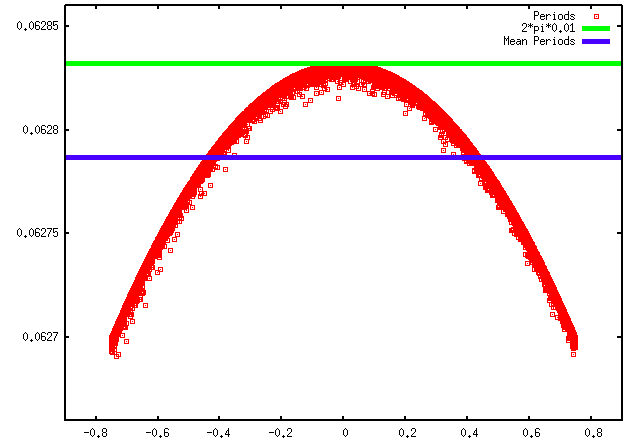
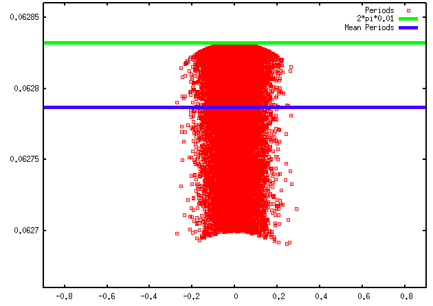
Figure 1: In red the computed periods with respect to the initial positions (at left) and to the initial velocities (at right). The case of $E_{\varepsilon}=-r^{3}$ with $\varepsilon=0.01$. In blue the mean of the periods, in green the $2\pi\varepsilon$ value.

In this section we consider the Vlasov equation (1.1) provided with the electric field given by (1.3) and with the initial condition (see [4])

$$f_{0}(r,v)=\frac{n_{0}}{\sqrt{2\pi}v_{th}}\exp\left(-\frac{v^{2}}{2v_{th}^{2}}\right)\chi_{[-0.75,0.75]}(r),$$ (2.9)

where the thermal velocity is $v_{th}=0.0727518214392$ and $\chi_{[-0.75,0.75]}(r)=1$ if $r\in[-0.75,0.75]$ and $0$ otherwise. In the particle approximation, we implement this distribution function with $N_{p}=20000$ macroparticles and equal weights $w_{i}=1/N_{p}$. Moreover, this initial condition will be used all along this work.

In this case, the characteristics equation or equivalently the Duffing equation (1.5) has periodic solutions in time (see the appendix). Thus, the time to make one rapid complete tour in the phase space depends only on the initial condition. It is actually constant in time and it corresponds to the period of the trajectory. The repartition of the periods with respect to the initial condition in (2.9) is given in Fig. 1. These values are computed with a fine RK4 solver and they are in accordance with formula (A.8) in the appendix. Notice that the periods are very close to $2\pi\varepsilon$, they belong to $(2\pi\varepsilon-1.5\varepsilon^{2},2\pi\varepsilon)$.

Now we compare the modified ETD scheme with a reference solution, obtained by solving (1.4) with explicit 4th order Runge-Kutta scheme with small time step. The solution in the phase space $(R,V)$ at different large times, obtained with $\varepsilon=0.01$, is illustrated in Fig. 2.

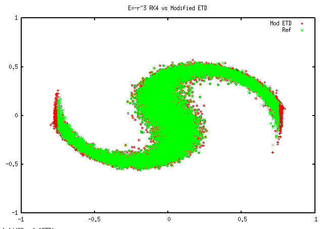
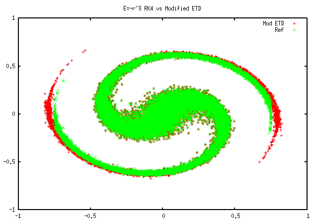
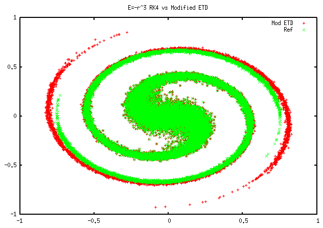
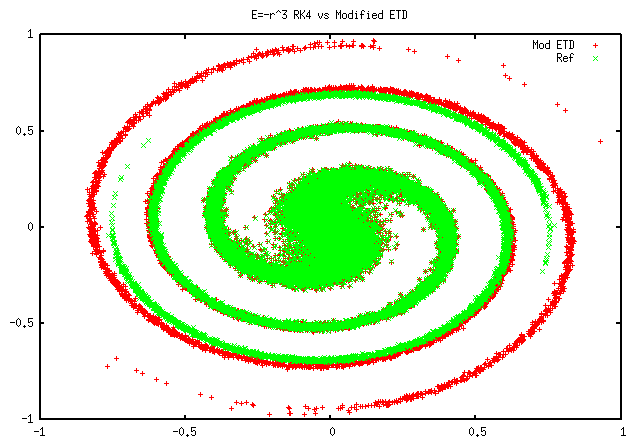
Figure 2: The case of $E_{\varepsilon}=-r^{3}$ with $\varepsilon=0.01$. In green: the reference solution obtained with a Runge-Kutta algorithm with time step $\Delta t=2\pi\varepsilon/100$. In red: the result of the modified ETD scheme with time step $\Delta t=0.5$. The final times are, from left to right and from top to bottom $t=10$, $20$, $30$ and $40$.

We notice that beyond $t=30$ the errors become significant. Next, we explain the reasons. Imagining a position (or velocity) trajectory in time being sinusoid-like, it is easy to see that a particle for which the period is underestimated (by the mean period) will drift inward in the phase space when applying the second step of the algorithm. When the period is overestimated, the particle will clearly drift outward. In addition, with the same approximation of the periods, larger is the amplitude of the sinusoid, bigger is the error made by the third step of the modified ETD scheme (see Fig. 3). Consequently, all the particles close to $(0,0)$ in the phase space are well treated by the algorithm, while the particles far from the center of the beam accumulate significant error in time. This behaviour was noticed in reference [3] in short time simulation, in terms of errors for particles off or on the slow manifold.

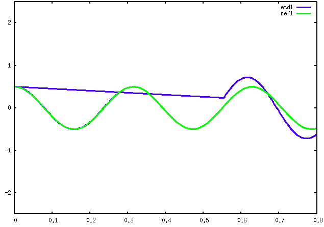
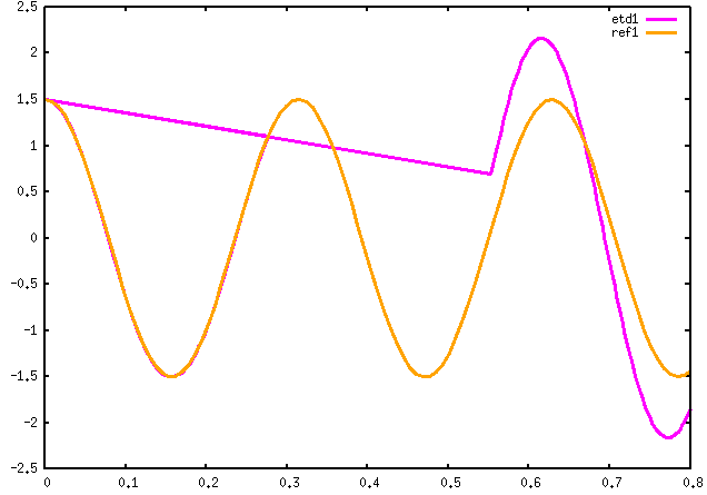
Figure 3: In green : the amplitude of the exact solution is $0.5$ and the period is $2\pi\varepsilon$. In blue the solution obtained with the ETD Scheme with a period $2\pi\varepsilon-15\varepsilon^{2}$. In orange : the amplitude of the exact solution is $1.5$ and the period is $2\pi\varepsilon$. In purple the solution obtained with the ETD Scheme with a period $2\pi\varepsilon-15\varepsilon^{2}$.

2.3 Application to long time simulation of the Vlasov-Poisson test case

In this section we consider the Vlasov-Poisson equation (1.2) provided with the initial condition (2.9). The calculus done in the appendix for computing periods is now difficult to achieve. Therefore, in this case, we compute the time to make one fast tour by using a fine RK4 solver. The Poisson equation is simply solved by means of the trapezoidal formula for the integral in $r$, with $256$ cells. As in the previous section, the fast time depends on the initial condition but in addition, it changes slowly in time. The same happens for the amplitude $\left\|\boldsymbol{y}\left(t\right)\right\|_{2}=\sqrt{R(t)^{2}+V(t)^{2}}$, see Figs. 5 and 6.

The comparison between the modified ETD scheme and a reference solution obtained with explicit 4th order Runge-Kutta scheme with small time step is summarized in Fig. 7. We see from Figs. 2 and 7 that the dynamics and/or the filamentation in the Vlasov-Poisson case is slower than that in the case of $E_{\varepsilon}$ given by (1.3). Certainly, this is because of bigger particle periods (compare Figs. 1 and 4)

Figure 4: In blue the computed periods with respect to the initial positions, in the Vlasov-Poisson case with $\varepsilon=0.01$. In red the mean of the periods, in green the $2\pi\varepsilon$ value.

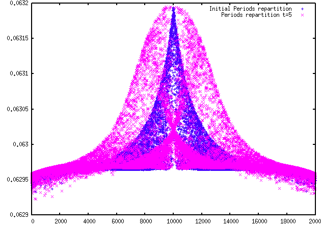
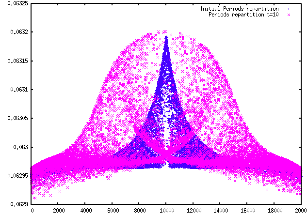
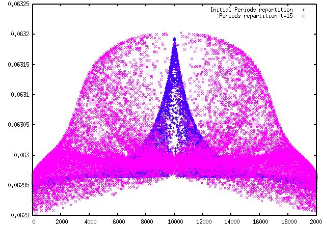
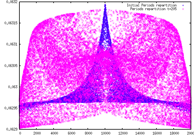
Figure 5: The periods distribution with respect to the initial periods (in blue) at times $t=5,10,15$, and $20$. The Vlasov-Poisson case with $\varepsilon=0.01$.

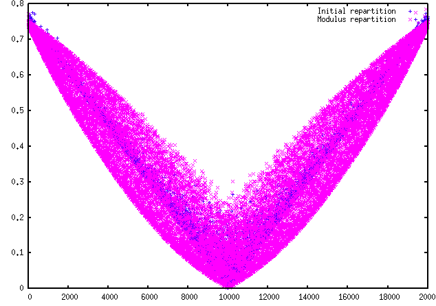
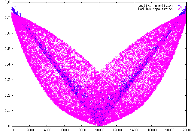
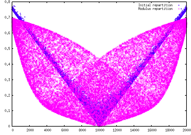
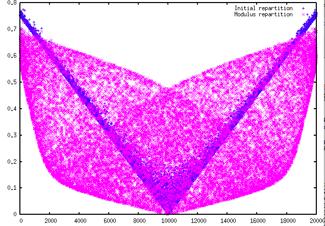
Figure 6: The modulus $\left\|\left(R\left(t\right),V\left(t\right)\right)\right\|_{2}$ with respect to the initial modulus (in blue) at times $t=5,10,15$, and $20$. The Vlasov-Poisson case with $\varepsilon=0.01$.

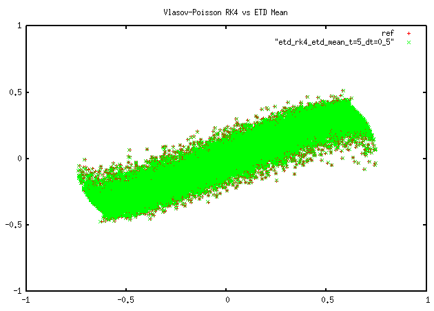
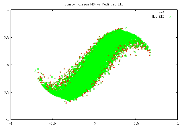
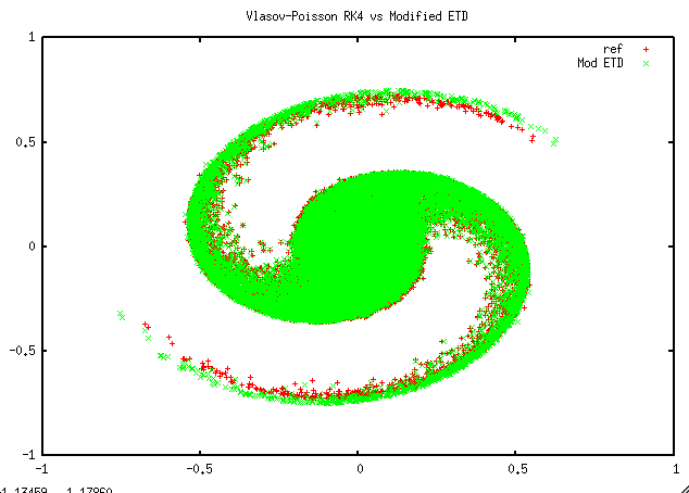
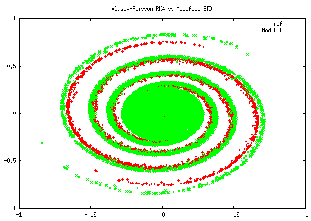
Figure 7: Vlasov-Poisson test case with $\varepsilon=0.01$. In red: the reference solution obtained with a Runge-Kutta algorithm with time step $\Delta t=2\pi\varepsilon/100$. In green: the result of the modified ETD scheme with time step $\Delta t=0.5$. The final times are, from left to right and from top to bottom: $t=5$, $10$, $30$ and $60$.

Now, we can recall the discussion from the previous section about the consequences of using approximated period within the second and the third steps of the algorithm. However, in this Vlasov-Poisson case, the periods distribution is more complicated and thus, it seems more difficult to clearly state how the approximation influences long time simulation. We only remark the following. The error done for particles at the extremities of the beam is less significant than in the previous Vlasov case. The reason is that the mean of the initial periods is very close to the periods of the particles far from the center of the beam (see Figs. 4 and 5). As for those close to the center $(0,0)$, we can see in Fig. 7 that particles slightly drifting both outward and inward are present, as expected from Fig. 4.

Therefore, in the next section we will compute at each time step the period of each particle, in order to take into account this slow evolution of the periods distribution. We recall that the slow evolution of the amplitudes is considered when applying the first step of the algorithm.

3 The new time-stepping scheme

In this section, we change Algorithm 2.1 by improving the approximation of each particle’s time to make one rapid complete tour. More precisely, within the first step, instead of solving the ODE (1.4) during some fixed fast time for all the particles, we will push each particle with its own fast time. Unfortunately, implementing this idea in Algorithm 2.1 will not work in the Vlasov-Poisson case. The reason is the following. Suppose that we have the particles $(\boldsymbol{y}_{i})_{i\in\{1,\dots,N_{p}\}}$ and their computed periods $(T_{i})_{i\in\{1,\dots,N_{p}\}}$ at time $t_{n}$. First, we finely solve the ODE with each particle as initial condition, during different times (the $T_{i}$s), paying attention to push enough in time (the maximum period) all the particles in order to calculate the correct self-consistent electric field. Then, applying the second step of Algorithm 2.1 with the corresponding $N_{i}$ will lead to particles at different times $t_{n}+N_{i}\,T_{i}$. Now, it is impossible to apply the third step of the algorithm, because the particles arrived at the minimum of $\big{(}t_{n}+N_{i}\,T_{i}\big{)}_{i\in\{1,\dots,N_{p}\}}$ can not be pushed with the right electric field since all the particles are not available at that time. This problem is solved by changing the steps of the algorithm, as it is described below, in Algorithm 3.4.

Firstly, note that dynamical system (1.4) can be rewritten as

$$\boldsymbol{y}^{\prime}\left(t\right)=\frac{1}{\varepsilon}M\boldsymbol{y}\left(t\right)+\boldsymbol{L}^{\varepsilon}\left(t,\boldsymbol{y}\left(t\right)\right),$$ (3.1)

where $\boldsymbol{y}$ is defined by (2.5) and $M$ and $\boldsymbol{L}^{\varepsilon}$ are given by

$$M=\left(\begin{array}[]{cc}~{}0&1\\ -1&0\end{array}\right)\quad\text{and}\quad\boldsymbol{L}^{\varepsilon}=\left(\begin{array}[]{c}0\\ E_{\varepsilon}\end{array}\right).$$ (3.2)

Let $T$ be a positive real number which is intended to be close to $2\pi$ and let $\boldsymbol{r}\left(\tau\right)$ be the matrix defined by

$$\boldsymbol{r}\left(\tau\right)=\left(\begin{array}[]{cc}~{}~{}\cos\big{(}\frac{2\pi}{T}\tau\big{)}&\sin\big{(}\frac{2\pi}{T}\tau\big{)}\\ -\sin\big{(}\frac{2\pi}{T}\tau\big{)}&\cos\big{(}\frac{2\pi}{T}\tau\big{)}\end{array}\right),$$ (3.5)

which is a $T$-periodic function. Then we compute

$$\frac{\text{d}}{\text{d}\tau}\left(\boldsymbol{r}\left(-\frac{\tau}{\varepsilon}\right)\boldsymbol{y}\left(\tau\right)\right) = \frac{2\pi}{\varepsilon T}\boldsymbol{r}\left(-\frac{\tau}{\varepsilon}\right)M\boldsymbol{y}\left(\tau\right)+\boldsymbol{r}\left(-\frac{\tau}{\varepsilon}\right)\left(\frac{1}{\varepsilon}M\boldsymbol{y}\left(t\right)+\boldsymbol{L}^{\varepsilon}\left(\tau,\boldsymbol{y}\left(\tau\right)\right)\right)$$ (3.6)

$$= \boldsymbol{r}\left(-\frac{\tau}{\varepsilon}\right)\boldsymbol{L}^{\varepsilon}\left(\tau,\boldsymbol{y}\left(\tau\right)\right)+\left(1-\frac{2\pi}{T}\right)\frac{1}{\varepsilon}\boldsymbol{r}\left(-\frac{\tau}{\varepsilon}\right)M\boldsymbol{y}\left(\tau\right)$$

$$= \boldsymbol{r}\left(-\frac{\tau}{\varepsilon}\right)\boldsymbol{\beta}^{\varepsilon}\left(\tau,\boldsymbol{y}\left(\tau\right)\right),$$

where

$$\boldsymbol{\beta}^{\varepsilon}\left(\tau,\boldsymbol{y}\left(\tau\right)\right)=\boldsymbol{L}^{\varepsilon}\left(\tau,\boldsymbol{y}\left(\tau\right)\right)+\left(1-\frac{2\pi}{T}\right)\frac{1}{\varepsilon}M\boldsymbol{y}\left(\tau\right).$$ (3.7)

Integrating (3.6) between $s$ and $t$ with $s<t$ thus leads to

$$\boldsymbol{y}\left(t\right)=\boldsymbol{r}\left(\frac{t-s}{\varepsilon}\right)\boldsymbol{y}\left(s\right)+\boldsymbol{r}\left(\frac{t-s}{\varepsilon}\right)\int_{s}^{t}\boldsymbol{r}\left(\frac{s-\tau}{\varepsilon}\right)\boldsymbol{\beta}^{\varepsilon}\left(\tau,\boldsymbol{y}\left(\tau\right)\right)d\tau.$$ (3.8)

Now we establish the time-stepping scheme. We write equation (3.8) with $s=t_{n}$ and $t=t_{n+1}=t_{n}+\Delta t$ in order to specify how the solution is computed at time $t_{n+1}$ from its known value at time $t_{n}$. Thus, for each particle of the beam we are faced with the numerical computation of the integral from $t_{n}$ to $t_{n+1}$ involved in the right hand side of (3.8). Subsequently, we denote by $\boldsymbol{y}_{i}$ the particle satisfying equation (3.1) provided with the initial condition $\boldsymbol{y}_{i}^{n}$. We denote by $T_{i}^{n}$ the time to make the first rapid complete tour starting at $t_{n}$. This time is computed numerically.

Since we want to build a scheme with a time step $\Delta t$ much larger than the fast oscillation, we first need to find the unique positive integers $N_{i}^{n}$ and the unique reals $o_{i}^{n}\in[0,T_{i}^{n})$ such that

$$\Delta t=N_{i}^{n}T_{i}^{n}+o_{i}^{n}.$$ (3.9)

The derivation of the scheme, Algorithm 3.4, is based on the following approximation.

Approximation 3.1.

We have for any $i\in\{1,\dots,N_{p}\}$

$$\int_{t}^{t+N_{i}^{n}T_{i}^{n}}\boldsymbol{r}^{n}_{i}\left(\frac{t-\tau}{\varepsilon}\right)\boldsymbol{\beta}^{\varepsilon}\left(\tau,\boldsymbol{y}_{i}\left(\tau\right)\right)d\tau\;\approx\;N_{i}^{n}\int_{t}^{t+T_{i}^{n}}\boldsymbol{r}^{n}_{i}\left(\frac{t-\tau}{\varepsilon}\right)\boldsymbol{\beta}^{\varepsilon}\left(\tau,\boldsymbol{y}_{i}\left(\tau\right)\right)d\tau$$ (3.10)

where $t=t_{n}+o_{i}^{n}$ and $\boldsymbol{r}_{i}^{n}$ corresponds to the matrix in (3.5) with $T=T_{i}^{n}/\varepsilon$.

Remark 3.2.

Approximation 3.1 is valid if we make the assumptions that the times for all particles to do the first rapid tour starting from $t$ evolve slowly in time and that the particle and the electric field evaluated at the particle position are quasi-periodic in time (with a period close to the time to make the first rapid complete tour).

Lemma 3.3.

Under Approximation 3.1 we obtain for any $i\in\{1,\dots,N_{p}\}$ and any time $t_{n}$

$$\boldsymbol{y}_{i}(t_{n+1})\approx\boldsymbol{y}_{i}(t_{n}+o_{i}^{n})+N_{i}^{n}\Big{(}\boldsymbol{y}_{i}({t_{n}+o_{i}^{n}+T_{i}^{n}})-\boldsymbol{y}_{i}(t_{n}+o_{i}^{n})\Big{)},$$ (3.11)

where $\boldsymbol{y}_{i}$ is the solution to equation (3.1) with a given initial condition $\boldsymbol{y}_{i}(t_{n})=\boldsymbol{y}_{i}^{n}$.

Proof.

Writing the variation-of-constants formula from $s=t_{n}+o_{i}^{n}$ to $t=t_{n+1}$ and recalling (3.9) we obtain the following exact scheme

$$\boldsymbol{y}_{i}(t_{n+1})=\boldsymbol{y}_{i}(t_{n}+o_{i}^{n})+\int_{t_{n}+o_{i}^{n}}^{t_{n+1}}\boldsymbol{r}_{i}^{n}\left(\frac{t_{n}+o_{i}^{n}-\tau}{\varepsilon}\right)\,\boldsymbol{\beta}^{\varepsilon}\left(\tau,\boldsymbol{y}_{i}\left(\tau\right)\right)d\tau$$ (3.12)

since $\boldsymbol{r}_{i}^{n}(N_{i}^{n}T_{i}^{n}/\varepsilon)$ is the identity matrix. Then, under Approximation 3.1 we obtain

$$\boldsymbol{y}_{i}(t_{n+1})\approx\boldsymbol{y}_{i}(t_{n}+o_{i}^{n})+N_{i}^{n}\int_{t_{n}+o_{i}^{n}}^{t_{n}+o_{i}^{n}+T_{i}^{n}}\boldsymbol{r}_{i}^{n}\left(\frac{t_{n}+o_{i}^{n}-\tau}{\varepsilon}\right)\boldsymbol{\beta}^{\varepsilon}\left(\tau,\boldsymbol{y}_{i}\left(\tau\right)\right)d\tau.$$ (3.13)

Applying now formula (3.8) with $s=t_{n}+o_{i}^{n}$, $t=t_{n}+o_{i}^{n}+T_{i}^{n}$ and $\boldsymbol{r}=\boldsymbol{r}_{i}^{n}$ yields

$$\boldsymbol{y}_{i}\left(t_{n}+o_{i}^{n}+T_{i}^{n}\right)-\boldsymbol{y}_{i}\left(t_{n}+o_{i}^{n}\right)=\int_{t_{n}+o_{i}^{n}}^{t_{n}+o_{i}^{n}+T_{i}^{n}}\boldsymbol{r}_{i}^{n}\left(\frac{t_{n}+o_{i}^{n}-\tau}{\varepsilon}\right)\boldsymbol{\beta}^{\varepsilon}\left(\tau,\boldsymbol{y}_{i}\left(\tau\right)\right)d\tau$$ (3.14)

since $\boldsymbol{r}_{i}^{n}(T_{i}^{n}/\varepsilon)$ is the identity matrix. Thus, injecting (3.14) in (3.13) leads to (3.11). ∎

Using Lemma 3.3, we deduce the following algorithm to compute $\boldsymbol{y}_{i}^{n+1}$ from $\boldsymbol{y}_{i}^{n}$.

Algorithm 3.4.

Assume that for each $i\in\{1,\dots,N_{p}\}$, $\boldsymbol{y}_{i}^{n}$, the value of a solution of (3.1) at time $t_{n}$, is given.

1. Compute from $(\boldsymbol{y}_{i}^{n})_{i\in\{1,\dots,N_{p}\}}$ the periods $(T_{i}^{n})_{i\in\{1,\dots,N_{p}\}}$ at time $t_{n}$.

2. For each $i\in\{1,\dots,N_{p}\}$ compute the unique positive integers $N_{i}^{n}$ and the unique reals $o_{i}^{n}\in[0,T^{n}_{i})$ such that

   $$\Delta t=N^{n}_{i}T^{n}_{i}+o^{n}_{i}.$$ (3.15)

3. For each $i\in\{1,\dots,N_{p}\}$ compute $\boldsymbol{y}_{i}(t_{n}+o^{n}_{i})$ and $\boldsymbol{y}_{i}(t_{n}+o_{i}^{n}+T_{i}^{n})$ by using a fine Runge-Kutta solver with initial condition $\boldsymbol{y}_{i}^{n}$.

4. For each $i\in\{1,\dots,N_{p}\}$ compute an approximation of $\boldsymbol{y}_{i}(t_{n+1})$ thanks to

   $$\boldsymbol{y}_{i}^{n+1}=\boldsymbol{y}_{i}(t_{n}+o^{n}_{i})+N_{i}\Big{(}\boldsymbol{y}_{i}(t_{n}+o_{i}^{n}+T_{i}^{n})-\boldsymbol{y}_{i}(t_{n}+o_{i}^{n})\Big{)}.$$ (3.16)

Remark 3.5.

As in [3], the way to compute the $(T_{i}^{n})_{i}$ from $(\boldsymbol{y}_{i}^{n})_{i}$ is the following. First, we solve the characteristics of equation (1.4) with a time step $(\Delta t)_{\!\text{RK}}=2\pi\varepsilon/100$, for all initial conditions $\boldsymbol{y}_{i}^{n}$ until all the particles reach their trajectory’s third extremum. The criterion for finding these extrema is the velocity’s change of sign. We then state that each particle’s period is the time interval between the first and the third extremum.

Remark 3.6.

The time step $(\Delta t)_{\!\text{RK}}$ chosen in the third step of the algorithm is $2\pi\varepsilon/100$. It is easy to see that the reals $(t_{n}+o_{i}^{n})_{i}$ and $(t_{n}+o_{i}^{n}+T_{i}^{n})_{i}$ are located on a few cells of length $(\Delta t)_{\!\text{RK}}$. Thus, we approximate the values $\boldsymbol{y}_{i}(t_{n}+o_{i}^{n})$ and $\boldsymbol{y}_{i}(t_{n}+o_{i}^{n}+T_{i}^{n})$ by quadratic interpolations.

4 Numerical simulations

We now do long time simulations with the improved ETD scheme (Algorithm 3.4) in the two cases of Vlasov equation. The results show that the new scheme works in long times while the modified ETD scheme becomes unstable. We can observe the idea underlined from the begining of the paper: using all along the simulation accurate approximations of each particle period leads to very accurate solutions. Thus, we note that the numerical solutions in the first case (Section 4.1) are very good since very precise values for the periods are available and in addition they do not change in time. On the contrary, in the Vlasov-Poisson case the periods are numerically approximated at several levels and therefore the scheme does not perform as well as in the first case.

4.1 Long time simulation of the undamped and undriven Duffing equation

In this section we consider the Vlasov equation (1.1) provided with the electric field given by (1.3) and with the initial condition (2.9). We recall that we use $20000$ macroparticles with equal weights.

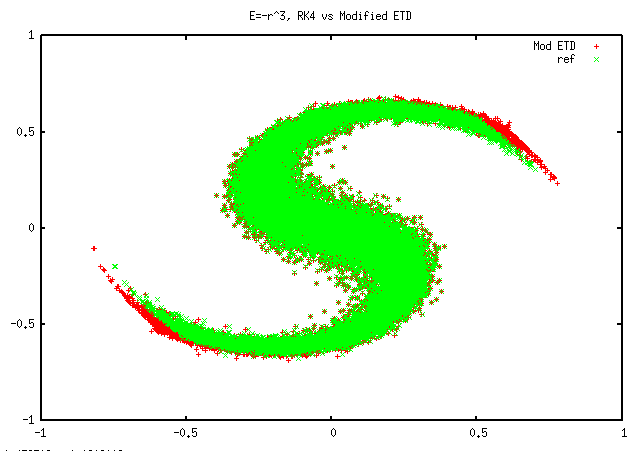
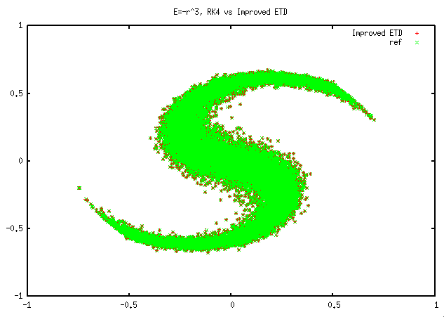
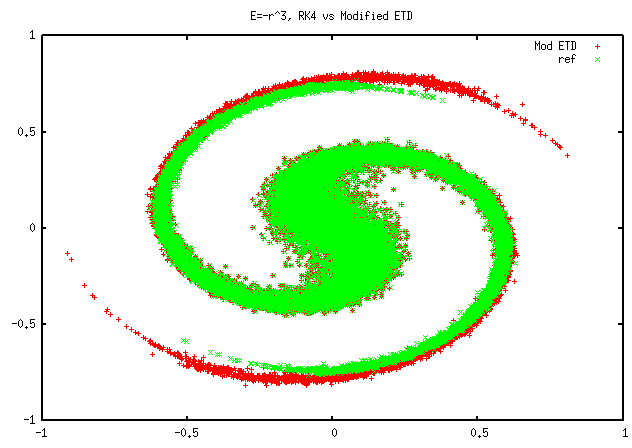
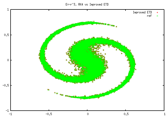
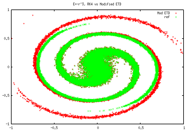
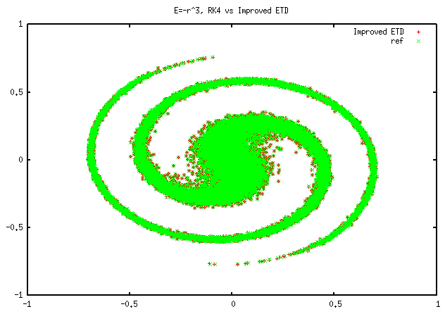
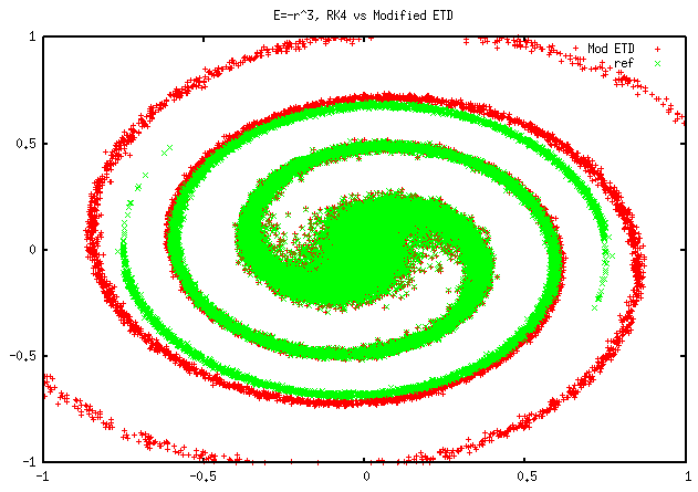
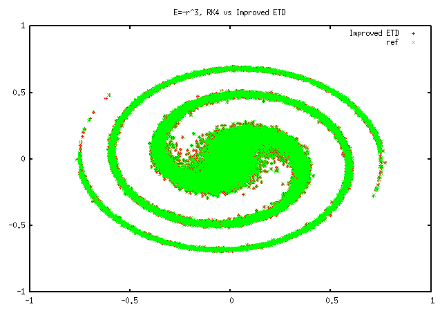
Figure 8: The case of $E_{\varepsilon}=-r^{3}$ with $\varepsilon=0.001$. In green: the reference solution. In red: the solution obtained with the modified ETD scheme (left) and with the improved ETD scheme (right). From top to bottom : $t=10$, $t=20$, $t=30$ and $t=37$. The time step used for the ETD schemes is $\Delta t=0.5$.

Note that the first step of Algorithm 3.4 is executed only initially, since the particle periods are constant in time.

The results obtained with $\varepsilon=0.001$ are summarized in Fig. 8 and with $\varepsilon=0.0001$ in Fig. 10 at right: we compare the outcome of the algorithm with a macroscopic time step $\Delta t=0.5$ to a reference solution computed with a small time step, $2\pi\varepsilon/100$. As already mentioned in Section 2.2 (see also the appendix), the particles moving according to (1.4) with given $E_{\varepsilon}$, have periodic trajectories and thus, the periods depend only on the initial conditions. We observe on Figs. 8 and 10 that both the filamentation phenomena and the fast rotation are well treated in long times by the improved ETD scheme (the old scheme is unstable at these times). Notice also that when $\varepsilon=0.0001$, the integers $N^{n}_{i}$ are about $800$, meaning that the ETD scheme is about $800$ times faster than the reference solution.

4.2 Long time simulation of the Vlasov-Poisson test case

In this section we consider the Vlasov-Poisson equation (1.2) provided with the initial condition (2.9). The Poisson equation is solved as mentioned in Section 2.3.

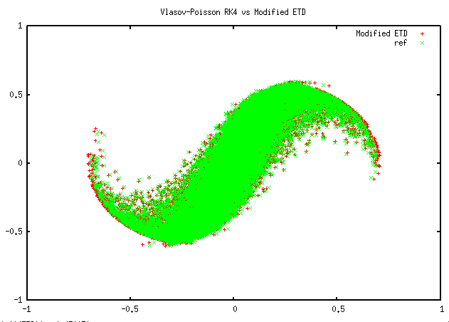
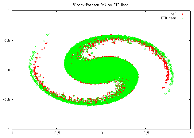
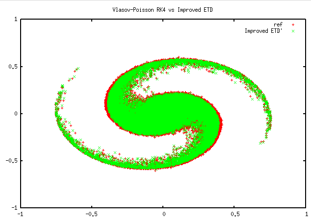
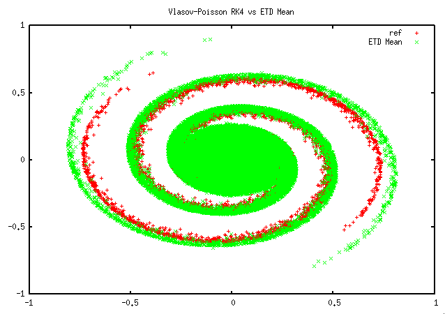
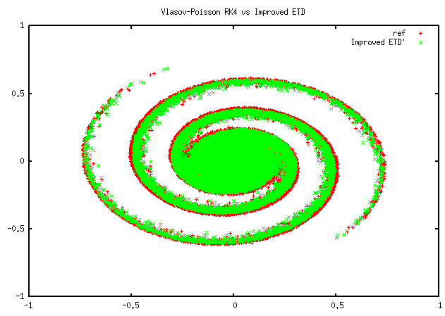
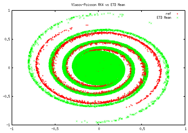
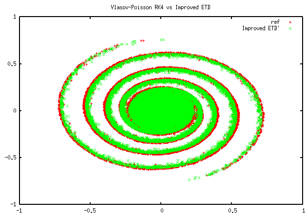
Figure 9: Vlasov-Poisson test case with $\varepsilon=0.001$. In red: the reference solution. In green: the solution obtained with the modified ETD scheme (left) and with the improved ETD scheme (right). From top to bottom : $t=15$, $t=30$, $t=45$ and $t=60$. The time step used for the ETD schemes is $\Delta t=0.5$.

The results obtained with $\varepsilon=0.001$ and the same time steps as above are summarized in Fig. 9. The case of $\varepsilon=0.0001$ is illustrated in Fig. 10 at left. Again, one can see the slower filamentation of the Vlasov-Poisson case in comparison with the given electric field case. The time to make one rapid complete tour evolves slowly in time (see Section 2.3). Therefore, the approximations made in Algorithm 3.4 lead to accurate results. In particular the particle filaments are well treated by the improved ETD scheme. Note again that the new algorithm is about $80$ times faster (when $\varepsilon=0.001$) than the reference solution.

Concluding, the scheme is able to produce quite accurate numerical solutions for stiff Vlasov type equations for different small values of $\varepsilon$ with the same computational cost, which is rather close to that of a reduced model.

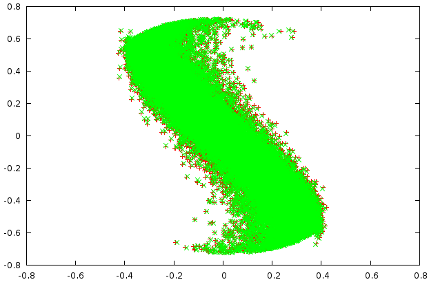
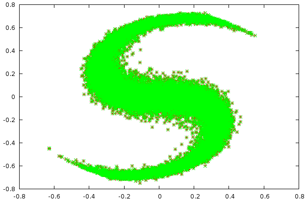
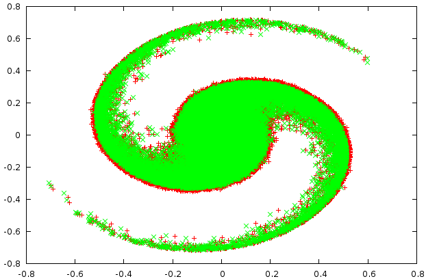
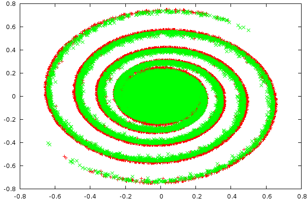
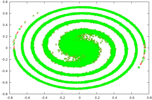
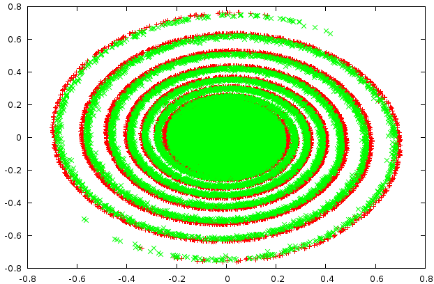
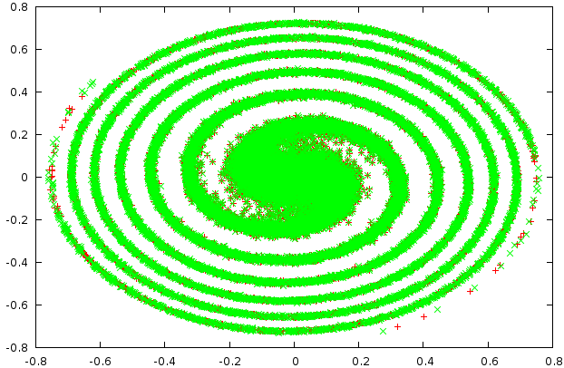
Figure 10: The cases of Vlasov-Poisson (left) and of Vlasov with $E_{\varepsilon}=-r^{3}$ (right), when $\varepsilon=0.0001$. In red: the reference solution. In green: the solution obtained with the improved ETD scheme. From top to bottom : $t=10$, $t=30$, $t=60$ and $t=90$. The time step for the ETD scheme is $\Delta t=0.5$.

Appendix A Appendix: Periods calculus for an undamped and undriven Duffing equation

Let $\varepsilon>0$ be some small parameter. The solution to the following Duffing-type equation

$$\left\{\begin{aligned} &R^{\prime\prime}+\frac{1}{\varepsilon^{2}}R+\frac{1}{\varepsilon}R^{3}=0\\ &R(0)=r_{0},~{}R^{\prime}(0)=v_{0}/\varepsilon\end{aligned}\right.$$ (A.1)

can be written by using Jacobi elliptic functions. In this appendix we obtain by elementary calculus (see [5]), an approximated value of order $3$ in $\varepsilon$ for the period of the solution. In particular, we obtain explicitly how the period $T$ depend on the initial condition $(r_{0},v_{0})$.

The orbits of the solutions are level curves of the Hamiltonian function

$${\cal H}(R,V)=\frac{R^{2}+\varepsilon^{2}V^{2}}{2\varepsilon^{2}}+\frac{R^{4}}{4\varepsilon},$$

where $V$ stands for $R^{\prime}$. As in Chapter V of reference [5], we denote the restoring force associated to the hard spring described by equation (A.1) by

$$g(R)=\frac{1}{\varepsilon^{2}}R+\frac{1}{\varepsilon}R^{3}$$

and by $G(R)=\cfrac{R^{2}}{2\varepsilon^{2}}+\cfrac{R^{4}}{4\varepsilon}$ the potential energy. Since the function $G$ has an absolute minimum in $(0,0)$ and no other critical point, all orbits are periodic. In addition, the closed orbit of a periodic solution is symmetric with respect to the $R$-axis and intersect it at two points, $(a,0)$ and $(b,0)$, with $a<b$. Taking into account that the function $g$ is odd, we have $a=-b$ and finally, we can determine an implicit formula for the period of the solution whose orbit intersect the $R$-axis in $(b,0)$:

$$T=4\int_{0}^{b}\frac{1}{\sqrt{2h-2G(R)}}dR,$$ (A.2)

where $h$ is the value of the Hamiltonian on the solution of system (A.1)

$$h=G(b)={\cal H}(r_{0},v_{0}).$$ (A.3)

Replacing $h$ in (A.2), we obtain

$$T=4\varepsilon\int_{0}^{1}\frac{1}{\sqrt{1-R^{2}+\frac{b^{2}\varepsilon}{2}(1-R^{4})}}dR.$$ (A.4)

Then, solving equation (A.3) for $b$ gives

$$b=\sqrt{\frac{1}{\varepsilon}\big{(}\sqrt{1+2\varepsilon(r_{0}^{2}+v_{0}^{2})+\varepsilon^{2}r_{0}^{4}}-1\big{)}},$$ (A.5)

which by Taylor expansion (recall $0<\varepsilon\ll 1$) results in

$$b^{2}\varepsilon=(r_{0}^{2}+v_{0}^{2})\varepsilon+\frac{r_{0}^{4}-(r_{0}^{2}+v_{0}^{2})^{2}}{2}\varepsilon^{2}+{\cal O}(\varepsilon^{3}).$$ (A.6)

Therefore, the parameter $\alpha=\cfrac{b^{2}\varepsilon}{2}$ is small when $\varepsilon\ll 1$. Thus, by Taylor expanding to second order the function

$$\alpha\mapsto\frac{1}{\sqrt{1-R^{2}+\alpha(1-R^{4})}}$$

for each $R$, we obtain the following approximation to the period

$$T=2\pi\varepsilon-\frac{3\pi}{4}b^{2}\varepsilon^{2}+\frac{57\pi}{128}b^{4}\varepsilon^{3}+{\cal O}(\varepsilon^{4}).$$ (A.7)

By injecting (A.6) in (A.7), we finally obtain

$$T = 2\pi\varepsilon-\frac{3\pi}{4}(r_{0}^{2}+v_{0}^{2})\varepsilon^{2}$$ (A.8)

$$+\left(\frac{105\pi}{128}(r_{0}^{2}+v_{0}^{2})^{2}-\frac{3\pi}{8}r_{0}^{4}\right)\varepsilon^{3}$$

$$+\,{\cal O}(\varepsilon^{4}).$$

References

- [1] C.K. Birdsall and A.B. Langdon. Plasma Physics via Computer Simulation. Institute of Physics, Bristol and Philadelphia, 1991.
- [2] S. M. Cox and P. C. Matthews. Exponential time differencing for stiff systems. J. Comput. Phys., 176:430–455, 2002.
- [3] E. Frénod, S. A. Hirstoaga, and E. Sonnendrücker. An exponential integrator for a highly oscillatory Vlasov equation. Discrete Contin. Dyn. Syst. Ser. S, 2014 (In Press).
- [4] E. Frénod, F. Salvarani, and E. Sonnendrücker. Long time simulation of a beam in a periodic focusing channel via a two-scale PIC-method. Math. Models Methods Appl. Sci., 19(2):175–197, 2009.
- [5] J. K. Hale. Ordinary differential equations. John Wiley, New York, 1969.
- [6] M. Hochbrück and A. Ostermann. Exponential integrators. Acta Numer., 19:209–286, 2010.
- [7] M. Lutz. Application of Lie Transform Techniques for simulation of a charged particle beam. Discrete Contin. Dyn. Syst. Ser. S, 2014 (In Press).