On multichannel solutions of nonlinear Schrödinger equations: algorithm, analysis and numerical explorations

Abstract.

We apply the method of modulation equations to numerically solve the NLS with multichannel dynamics, given by a trapped localized state and radiation. This approach employs the modulation theory of Soffer-Weinstein, which gives a system of ODE’s coupled to the radiation term, which is valid for all times. We comment on the differences of this method from the well-known method of collective coordinates.

1. Introduction

A wide class of conservative nonlinear dispersive equations, such as nonlinear Schrödinger equations and Korteweg-de Vries equations (See e.g. the reviews [10, 25] ), admit solutions with more than one channel or the multichannel solutions, which means that the asymptotic behavior of the solution is given by a linear combination of a localized (in space), periodic (in time) wave (solitary or standing wave) and a dispersive part. The multichannel solutions are important and useful in both theoretical analysis and applications. For example, they occur frequently in the nonlinear scattering theory in the study of nonintegrable equations and the design of absorbing boundary conditions for the partial differential equations. They also frequently appear in various nonlinear systems, such as quantum waves and nonlinear optics. In general, the dynamics is complicated due to the interaction between the coherent structures and the radiation around.

Among the analytical approaches to study the multichannel solutions, the collective coordinate approach is one of the most useful tools, see a detailed review in [11]. The collective coordinate approach, see e.g. [1, 2, 3, 5, 21, 22, 24, 32], approximates the solution at any given time, by the nearest soliton structure possible; this gives ODE’s for the dynamics of the soliton(s) parameters, which decouple from the rest of the system. This method is very effective in predicting the dynamics of solitons in nonlinear systems [17, 18, 19, 20] and has some other applications like in [33], but it does not take the radiations into consideration. In 1990, A. Soffer and M. I. Weinstein rigorously established the mathematical theory and derived the governing dynamical equations for the multichannel solutions in general system when they were studying the scattering in nonintegrable equations [26]. The governing equations of the multichannel solutions can fully describe the dynamics of the solitary wave and the dispersive part simultaneously, and they are known as modulation equations in literature. However, little numerical aspects have been done to the study of the multichannel solutions by modulation equations approach so far. In this work, we focus on the multichannel solutions in the nonlinear Schrödinger (NLS) equations in $d$ dimensions($d=1,2,3$), i.e.

(1.1) $$i\partial_{t}\Phi(\mathbf{x},t)=\left[-\Delta+V(\mathbf{x})+\lambda|\Phi|^{2m}\right]\Phi(\mathbf{x},t),\quad\mathbf{x}\in\mathbb{R}^{d},\ t>0,$$

(1.2) $$\Phi(\mathbf{x},0)=\Phi_{0}(\mathbf{x}),\quad\mathbf{x}\in\mathbb{R}^{d},$$

where $m\in\mathbb{N}$, $\lambda\in\mathbb{R}$ and $0<|\lambda|\ll 1$, $\Phi_{0}(\mathbf{x})$ is the given initial data and $V(\mathbf{x})$ is the real-valued potential function such that $-\Delta+V$ has continuous spectrum. It is well-known that mass of system $M$ and the Hamiltonian (energy) of the system $H$ are conserved, i.e.

(1.3) $$M(t) := \int_{\mathbb{R}^{d}}\left|\Phi(\mathbf{x},t)\right|^{2}\mathrm{d}\mathbf{x}\equiv M(0),$$

(1.4) $$H(t) := \int_{\mathbb{R}^{d}}\left[\left|\nabla\Phi(\mathbf{x},t)\right|^{2}+V(\mathbf{x})\left|\Phi(\mathbf{x},t)\right|^{2}+\frac{\lambda}{m+1}\left|\Phi(\mathbf{x},t)\right|^{2m+2}\right]\mathrm{d}\mathbf{x}$$

$$\equiv H(0).$$

Based on the modulation equations of the NLS provided in [26], accurate numerical algorithms are proposed, analyzed and applied to explore the multichannel solutions numerically. In the study, the key and necessary step for the numerical algorithm of modulation equations is to solve the nonlinear eigenvalue problems of the NLS in the case of continuous spectrum, which to our best knowledge, no applicable numerical methods are available in literature. For this problem, the existing numerical methods only consider either the ground state of the NLS or the excited states in case of discrete spectrum [7, 8, 12]. Thus, before we design the algorithm for the modulation equations, we propose and analyze a new effective numerical method for solving the eigenvalue problem of the NLS with continuous spectrum.

The rest of the paper is organized as follows. In Section 2, we shall give a brief review of the multichannel solutions of the NLS. In Section 3, we shall propose and analyze the algorithm for the nonlinear eigenvalue problem of the NLS. The algorithm for the modulation equations is given in Section 4 followed by numerical explorations.

2. Review of multichannel solutions

In this section, we shall formally derive the modulation equations of the NLS and review some related mathematical theories for the readers’ convenience. Comments on the differences of this method from the well-known method of collective coordinates are given in the end.

2.1. Formal derivations of modulation equations

Based on the simple physical observation that if one starts with the linear Schrödinger equation which describes a bound state and a dispersive wave (corresponding to the continuous spectral part of the Hamiltonian), then the qualitative behavior should not change that much in response to a small nonlinear and Hamiltonian perturbation in the dynamics, i.e. we should still see a localized part which decouples after a long time from the dispersive part, we take the ansatz of the solution of (1.1) [26] as

(2.1) $$\Phi(\mathbf{x},t)=\mathrm{e}^{-i\theta(t)}\left(\psi_{E(t)}(\mathbf{x})+\phi(\mathbf{x},t)\right),\quad\mathbf{x}\in\mathbf{R}^{d},\ \,t\geq 0,$$

(2.2) $$\theta(t)=\int_{0}^{t}E(s)\mathrm{d}s-\gamma(t),\quad t\geq 0,$$

with initial conditions

$$\Phi_{0}(\mathbf{x})=\mathrm{e}^{-i\theta_{0}}\left(\psi_{E_{0}}(\mathbf{x})+\phi_{0}(\mathbf{x})\right),$$

(2.3) $$E(0)=E_{0},\quad\gamma(0)=\gamma_{0},\quad\phi(\mathbf{x},t=0)=\phi_{0}(\mathbf{x}).$$

Here, $\psi_{E}(\mathbf{x})$ is the nonlinear bound state of NLS (1.1) with eigenvalue $E$, i.e.

(2.4) $$\left[-\Delta+V(\mathbf{x})+\lambda\psi_{E}^{2m}(\mathbf{x})\right]\psi_{E}(\mathbf{x})=E\psi_{E}(\mathbf{x}),\quad\mathbf{x}\in\mathbb{R}^{d},$$

$$\psi_{E}\in H^{2}(\mathbb{R}^{d}),\qquad\psi_{E}>0,$$

which is the localized part in the multichannel solution. $\phi$ is the dispersive wave and $\gamma\in\mathbb{R}$ is the frequency. Also, we assume the orthogonality condition:

(2.5) $$\left<\psi_{E_{0}},\phi_{0}\right>=0,\quad\frac{\mathrm{d}}{\mathrm{d}t}\left<\psi_{E_{0}},\phi(t)\right>=0,$$

where the inner product $<u,v>:=\int_{\mathbb{R}^{d}}\bar{u}v\,\mathrm{d}\mathbf{x}$ for functions $u$ and $v$, with $\bar{u}$ the complex conjugate of $u$. Condition (2.5) immediately implies that $\left<\psi_{E_{0}},\phi(t)\right>=0$.

Plugging ansatz (2.1) into the NLS (1.1) and noting (2.4), we get

$$i\partial_{t}\phi(\mathbf{x},t)= \left[-\Delta+V-E(t)+\dot{\gamma}(t)\right]\phi+\lambda\left|\psi_{E(t)}+\phi\right|^{2m}\left(\psi_{E(t)}+\phi\right)$$

$$-\lambda\psi_{E(t)}^{2m+1}+\dot{\gamma}(t)\psi_{E(t)}-i\dot{E}(t)\partial_{E}\psi_{E(t)},$$

where from (2.4) we have

(2.7) $$\left[-\Delta+V+(2m+1)\lambda\psi_{E}^{2m}-E\right]\partial_{E}\psi_{E}=\psi_{E}.$$

Denote

(2.8a) $$F_{1}=\dot{\gamma}\psi_{E}-i\dot{E}\partial_{E}\psi_{E},$$

(2.8b) $$F_{2}=\lambda\left|\psi_{E}+\phi\right|^{2m}\left(\psi_{E}+\phi\right)-\lambda\psi_{E}^{2m+1}-\lambda\psi_{E_{0}}^{2m}\phi,$$

then (2.1) becomes,

$$i\partial_{t}\phi(\mathbf{x},t)= \left(-\Delta+V+\lambda\psi_{E_{0}}^{2m}\right)\phi+\left(\dot{\gamma}-E\right)\phi+F_{1}+F_{2}.$$

Taking the inner product on both sides of the above equation with $\psi_{E_{0}}$, we get

$$i\left<\partial_{t}\phi,\psi_{E_{0}}\right>= \left<(-\Delta+V+\lambda\psi_{E_{0}}^{2m})\phi,\psi_{E_{0}}\right>+\left(\dot{\gamma}-E\right)\left<\phi,\psi_{E_{0}}\right>$$

$$+\left<F_{1}+F_{2},\psi_{E_{0}}\right>.$$

Using (2.4) and the orthogonal condition (2.5), then noting (2.8a) we get

$$\left<F_{2},\psi_{E_{0}}\right>=-\left<F_{1},\psi_{E_{0}}\right>=-\dot{\gamma}\left<\psi_{E},\psi_{E_{0}}\right>-i\dot{E}\left<\partial_{E}\psi_{E},\psi_{E_{0}}\right>.$$

Taking the real part and imaginary part of the above equation, respectively, we get

$$\dot{\gamma}(t)=-\frac{\mathfrak{R}\left<F_{2},\psi_{E_{0}}\right>}{\left<\psi_{E},\psi_{E_{0}}\right>},\qquad\dot{E}(t)=-\frac{\mathfrak{I}\left<F_{2},\psi_{E_{0}}\right>}{\left<\partial_{E}\psi_{E},\psi_{E_{0}}\right>},$$

where $\mathfrak{R}z$ and $\mathfrak{I}z$ denote the real part and imaginary part of a complex number $z$, respectively. Together with (2.1), we get the modulation equations for the dynamics of multichannel solutions as the coupled system

(2.9a) $$i\partial_{t}\phi(\mathbf{x},t)=\left[-\Delta+V-E(t)+\dot{\gamma}(t)\right]\phi+\lambda\left|\psi_{E(t)}+\phi\right|^{2m}\left(\psi_{E(t)}+\phi\right)$$

$$\qquad\qquad\quad\,-\lambda\psi_{E(t)}^{2m+1}+\dot{\gamma}(t)\psi_{E(t)}-i\dot{E}(t)\partial_{E}\psi_{E(t)},\quad\mathbf{x}\in\mathbb{R}^{d},\ \,t>0,$$

(2.9b) $$\dot{\gamma}(t)=-\frac{\mathfrak{R}\left<F_{2},\psi_{E_{0}}\right>}{\left<\psi_{E},\psi_{E_{0}}\right>},\quad t>0,$$

(2.9c) $$\dot{E}(t)=-\frac{\mathfrak{I}\left<F_{2},\psi_{E_{0}}\right>}{\left<\partial_{E}\psi_{E},\psi_{E_{0}}\right>},\quad t>0,$$

with initial conditions (2.3). Components $E$ and $\gamma$ are sometimes referred as collective coordinates in physics, and the dispersive term $\phi$ are related to radiations.

2.2. Review on theoretical results

Here always assume the linear operator $-\Delta+V$ has continuous spectrum but with exactly one bound state (isolated eigenvalue) on $L^{2}(\mathbb{R}^{d})$ with strictly negative eigenvalue $E_{*}$. In fact, the nonlinear eigenvalue problem (2.4) and the coupled modulation equations (2.9) have been well-studied by A. Soffer and M. I. Weinstein in [26]. Here we will briefly state some main results established there on the eigenvalue problem and the modulation equations. For the detailed theoretical statements and proofs, we refer the readers to [26].

For the nonlinear eigenvalue problem

For any $E\in(E_{*},0)$ if $\lambda>0$ (defocusing case), and for any $E<E_{*}$ if $\lambda<0$ (focusing case), the nonlinear eigenvalue problem (2.4) has a unique positive solutions in $H^{2}(\mathbb{R}^{d})$.

For the modulation equations

(Global well-posedness) For initial conditions $\phi(\mathbf{x},0)=\phi_{0}(\mathbf{x})\in H^{1}(\mathbb{R}^{d})$, $\gamma(0)=\gamma_{0}\in\mathbb{R}$, and $E(0)=E_{0}\in\mathbb{R}$, where $E_{0}\in(E_{*},0)$ if $\lambda>0$ and $E_{0}<E_{*}$ if $\lambda<0$, the modulation equations (2.9) has a unique solution $E(t),V(t)\in C^{1}[0,\infty)$ and $\phi\in C([0,\infty);H^{1}).$

(Dynamical property) For $0<t<\infty$, the solutions $E(t)\in(E_{*},0)$ if $\lambda>0$ and $E(t)<E_{*}$ if $\lambda<0$. As $t\to\infty,$ there exist two constants $\tilde{E},\tilde{\gamma}$, such that $E(t)\to\tilde{E}$, $\gamma(t)\to\tilde{\gamma}$.

2.3. Relation of modulation equations to collective coordinates

The method of modulation equations described above is closely related to the method of collective coordinates. In fact, it was proven in [26] that if the solution at any time is close to a soliton, then it can be written as a soliton plus small remainder which is also orthogonal in the above sense. Hence, both methods give a decomposition with small corrections. However, the method of the modulation equations also give a PDE for the radiation term, and coupling between the radiation and the ODE’s. Hence the modulation equations approach allows : (i) Control of the error in the ODE’s. (ii) Allows approximating the effect of radiation on the soliton dynamics, either exactly, or by using a good approximation of the coupling term. (iii) When the radiation effect is critical, as in dissipation mediated processes by the radiation [27, 28], one can derive the leading dissipation (radiation mediated!) term from the coupled equations, and find the leading behavior for processes in which a soliton changes state, for example from excited to ground state. (see [28, 29]). (iv) Resolving the soliton part as it arrives at the boundary of the domain of computation. This can not be handled by absorbing boundaries [30]. (v) Allows the rigorous asymptotic stability and scattering over arbitrary large time intervals.

3. On the nonlinear eigenvalue problem

In order to solve the modulation equations (2.9) at time $t$, we notice that we need to compute the bound state $\psi_{E(t)}$ which is the solution of the nonlinear eigenvalue problem (2.4). Thus, in this section, we shall propose and analyze an efficient algorithm to compute the bound state of (2.4) who has continuous spectrum.

3.1. Numerical method

For a given $E$ within the spectrum, since the bound state decays very fast to zero at far field, we truncate problem (2.4) onto a finite interval $\Omega=[-L,L]^{d}$ and impose the homogeneous Dirichlet boundary condition for numerical aspects, i.e.

(3.1a) $$\left[-\Delta+V(\mathbf{x})+\lambda\psi_{E}^{2m}(\mathbf{x})\right]\psi_{E}(\mathbf{x})=E\psi_{E}(\mathbf{x}),\quad\mathbf{x}\in\Omega,$$

(3.1b) $$\psi_{E}(\mathbf{x})=0,\quad\mathbf{x}\in\partial\Omega.$$

The algorithm reads as the following. Denote $\psi^{(n)}_{E}(n=0,1,\ldots,)$ as the approximation to $\psi_{E}$ and suppose $\psi^{(0)}_{E}$ is the initial guess, then $\psi_{E}^{(n+1)}$ is updated as:

Step 1 Find the ground state of the Hamiltonian functional

$$H^{n}(\psi)=\int_{\Omega}\left(|\nabla\psi|^{2}+V|\psi|^{2}+\lambda\left|\psi_{E}^{(n)}\right|^{2m}\cdot|\psi|^{2}\right)\mathrm{d}\mathbf{x},$$

in the unit sphere of $L^{2}(\Omega)$. Denote the solution as

(3.2) $$\widetilde{\psi}_{E}^{(n+1)}:=\arg\min\{H^{n}(\psi):\psi\in L^{2}(\Omega),\ \|\psi\|_{L^{2}}=1\}.$$

Step 2 Scale the ground state $\widetilde{\psi}_{E}^{(n+1)}$ according to the energy $E$. That is to find the scaling constant $c^{n}$ such that

(3.3) $$\psi_{E}^{(n+1)}:=c^{n}\widetilde{\psi}_{E}^{(n+1)},$$

satisfies

$$\int_{\Omega}\left[\left|\nabla\psi_{E}^{(n+1)}\right|^{2}+V\left|\psi_{E}^{(n+1)}\right|^{2}+\lambda\left|\psi_{E}^{(n+1)}\right|^{2m+2}\right]\mathrm{d}\mathbf{x}=E\left\|\psi_{E}^{(n+1)}\right\|_{L^{2}}^{2},$$

where we obtain

$$c^{n}=\left|\frac{E-\int_{\Omega}\left[\left|\nabla\widetilde{\psi}_{E}^{(n+1)}\right|^{2}+V\left|\widetilde{\psi}_{E}^{(n+1)}\right|^{2}\right]\mathrm{d}\mathbf{x}}{\lambda\int_{\Omega}\left|\widetilde{\psi}_{E}^{(n+1)}\right|^{2m+2}\mathrm{d}\mathbf{x}}\right|^{\frac{1}{2m}}.$$

For the first step, we use the normalized gradient flow method with a backward Euler sine pseudospectral discretization [7, 8] to get the ground state $\widetilde{\psi}_{E}^{(n+1)}$. For the second step, we use the standard sine pseudospectral discretization [14, 31] for the spatial derivative and integrations. Once $\psi_{E}$ is obtained, $\partial_{E}\psi_{E}$ can be found out from (2.7) with zero boundary conditions on $\Omega$ by the sine pseudospectral discretization.

3.2. Convergence analysis

For the proposed algorithm (3.2)-(3.3), we have the convergence result stated as the following theorem.

Theorem 3.1.

For the iteration algorithm (3.2)-(3.3) for solving the eigenvalue problem (3.1), if $\psi_{E}^{(0)}$ is sufficiently close to $\psi_{E}$ in $H^{1}(\Omega)$, we have

(3.4) $$\left\|\psi_{E}^{(n)}-\psi_{E}\right\|_{H^{1}(\Omega)}\rightarrow 0,\qquad n\rightarrow\infty.$$

The proof of the convergence theorem is given by the following steps. Let $\psi_{0}$ with $\|\psi_{0}\|_{L^{2}}=1$ be the ground state of $-\Delta+V(\mathbf{x})$ on $L^{2}(\mathbf{R})$ with the eigenvalue $E_{*}<0$. For simplicity, we work in the one space dimension case, i.e. $d=1,\ \mathbf{x}=x$. Furthermore, we assume that $E$ is in some small neighborhood of $E_{*}$ to be determined, and we use the $\psi_{E}^{0}=\psi_{0}$ as the initial guess for the iteration scheme. For general cases, the argument can proceed in a similar way. Define the functional, which is the scaling step used in (3.3)

$$\eta_{E}:\psi(\in H^{1})\to\mathbb{R}^{1},$$

$$\eta_{E}(\psi):=\frac{E-\int|\psi|^{2}\mathrm{d}x-\int\left(|\nabla\psi|^{2}+V|\psi|^{2}\right)\mathrm{d}x}{\lambda\int|\psi|^{2m+2}\mathrm{d}x},\quad\mbox{and}\quad\widetilde{\eta}_{E}(\psi):=\left|\eta_{E}(\psi)\right|^{\frac{1}{2m}}.$$

Proposition 3.1.

The following three facts are true.

a) $\eta_{E}(\psi_{0})=\frac{E-E_{*}}{\lambda\int|\psi_{0}|^{2m+2}\mathrm{d}x}.$

b) Suppose $\|\psi-\psi_{0}\|_{H^{1}}\leq b\ll 1,$ then

$$|\eta_{E}(\psi)|\leq|\eta_{E}(\psi_{0})|+C|E-E_{*}|\|\psi-\psi_{0}\|_{H^{1}}+C\|\psi-\psi_{0}\|_{H^{1}}\|\psi-\psi_{0}\|_{L^{2}}.$$

c) For $\|\psi-\psi_{0}\|_{H^{1}}+\|\psi^{\prime}-\psi_{0}\|_{H^{1}}\leq 2b$,

$$|\eta_{E}(\psi)-\eta_{E}(\eta^{\prime})|\leq C|E-E_{*}|\|\psi-\psi^{\prime}\|_{H^{1}}+O(\|\psi-\psi_{0}\|_{H^{1}}+\|\psi^{\prime}-\psi_{0}\|_{H^{1}})\|\psi-\psi^{\prime}\|_{L^{2}}.$$

Proof of Proposition 3.1:

a) Since $\psi_{0}$ is normalized to $1$ in $L^{2}$ and $-\Delta\psi_{0}+V\psi_{0}=E_{*}\psi_{0},$ so

$$\eta_{E}(\psi_{0})=\frac{E-\int\left(|\nabla\psi_{0}|^{2}+V|\psi_{0}|^{2}\right)\mathrm{d}x}{\lambda\int|\psi_{0}|^{2m+2}\mathrm{d}x}=\frac{E-E_{*}}{\lambda\int\psi_{0}^{2m+2}\mathrm{d}x}.$$

b) Expand $\eta_{E}(\psi)$ around $\psi_{0}$:

$$\eta_{E}(\psi)= \eta_{E}(\psi_{0})+\frac{\delta\eta}{\delta\psi}\big{|}_{\psi=\psi_{0}}(\psi-\psi_{0})+\frac{\delta^{2}\eta}{\delta\psi_{i}\delta\psi_{j}}\big{|}_{\psi=\psi_{0}}(\psi_{i}-\psi_{0})(\psi_{j}-\psi_{0})$$

$$+O((\psi-\psi_{0})^{2}),$$

where $\psi_{i}=\psi$ or $\psi^{*}$. At the ‘point’ $\psi_{0}$, by definition of the ground state, we have

$$\frac{\delta\eta}{\delta\psi}\big{|}_{\psi=\psi_{0}} =\frac{1}{\lambda\int|\psi_{0}|^{2m+2}\mathrm{d}x}\frac{\delta}{\delta\psi}\{E(\psi,\psi)-(\psi,H_{0}\psi)\}$$

$$\quad+\frac{E(\psi_{0},\psi_{0})-(\psi_{0},H_{0}\psi_{0})}{\lambda(\int|\psi_{0}|^{2m+2}\mathrm{d}x)^{2}}\frac{\delta}{\delta\psi}\int|\psi|^{2m+2}\mathrm{d}x$$

$$=\frac{(E-E_{*})<\psi_{0}|+\frac{E-E_{*}}{\int|\psi_{0}|^{2m+2}\mathrm{d}x}C_{m}<|\psi_{0}|^{m}\psi_{0}^{*}|}{\lambda\int|\psi_{0}|^{2m+2}\mathrm{d}x},$$

where $H_{0}=-\Delta+V+\lambda\psi_{0}^{2m}$, and $<\phi|$ stands for the operator $<\phi|f=\int\phi^{*}f\mathrm{d}x.$ Therefore,

$$\left|\frac{\delta\eta}{\delta\psi}\big{|}_{\psi=\psi_{0}}(\psi-\psi_{0})\right|\leq\frac{C_{m}+1}{|\lambda|\int|\psi_{0}|^{2m+2}\mathrm{d}x}|E-E_{*}|\left\|\psi\right\|_{L^{2}}\|\psi-\psi_{0}\|_{H^{1}}.$$

The higher order terms are similarly controlled, where we use that

$$\|\psi_{i}-\psi_{0}\|_{L^{\infty}}\leq C\|\psi_{i}-\psi_{0}\|_{H^{1}}.$$

c) Using the expansion in b), we have that

$$\eta_{E}(\psi)-\eta_{E}(\psi^{\prime})=\frac{\delta\eta}{\delta\psi}\big{|}_{\psi=\psi_{0}}(\delta\psi-\delta\psi^{\prime})+O(\delta\psi^{2}-\delta(\psi^{\prime})^{2}),$$

where $\delta\psi=\psi-\psi_{0}$, $\delta\psi^{\prime}=\psi^{\prime}-\psi_{0}.$ Hence,

$$\quad\left|\eta_{E}(\psi)-\eta_{E}(\psi^{\prime})\right|$$

$$\leq\frac{C}{|\lambda|\int|\psi_{0}|^{2m+2}\mathrm{d}x}\Big{[}|E-E_{*}|(\|\psi\|_{H^{1}}+\|\psi^{\prime}\|_{H^{1}}+1)\|\psi-\psi^{\prime}\|_{L^{2}}$$

$$\quad+\|\psi-\psi^{\prime}\|_{L^{2}}O(\|\psi-\psi_{0}\|_{H^{1}}+\|\psi^{\prime}-\psi_{0}\|_{H^{1}})\Big{]}.$$

Then the proof of the proposition is completed.

$\square$

Now, we can proceed to the proof of the convergence of the scheme, which is similar to the way used in [4].

Proof of Theorem 3.1 We need to show that the mapping defined by the iteration scheme is a strict contracting mapping for $|E-E_{*}|$ sufficiently small, on a complete metric space containing $\psi_{0}$ as an internal point. So we choose the metric space $\mathcal{M}_{0,\varepsilon}$ to be

$$\mathcal{M}_{0,\varepsilon}:=\left\{\psi\in H^{1}|\,\left\|\psi-\psi_{0}\right\|\leq\varepsilon,\ \|\psi\|_{L^{2}}=1\right\}.$$

Now, $\psi_{0}\in\mathcal{M}_{0,\varepsilon}$. Hence, for any $\psi\in\mathcal{M}_{0,\varepsilon}$, we have that

$$|\lambda\eta_{E}(\psi)| \leq|\lambda||\eta_{E}(\psi)-\eta_{E}(\psi_{0})|+\lambda\eta_{E}(\psi_{0})$$

$$\leq C(\psi_{0},\varepsilon)|E-E_{*}|\|\psi-\psi_{0}\|_{L^{2}}+C(\psi_{0})|E-E_{*}|$$

$$\quad+C\|\psi-\psi_{0}\|_{H^{1}}\|\psi-\psi_{0}\|_{L^{2}}$$

$$\leq C(\psi_{0},\varepsilon)|E-E_{*}|\varepsilon+C(\psi_{0})|E-E_{*}|+O(\varepsilon^{2}).$$

Define the map $S:\mathcal{M}_{0,\varepsilon}\to H^{1}$ by

$$S(\psi):=\frac{P_{g}^{\psi}\psi_{0}}{\|P_{g}^{\psi}\psi_{0}\|_{L^{2}}},$$

where $P_{g}^{\psi}$ denotes the projection on the ground state of the Hamiltonian:

$$H_{\psi}:=-\Delta+V+\lambda\eta_{E}(\psi)|\psi|^{2m}.$$

Clearly, $\|S(\psi)\|_{L^{2}}=1$, and $S(\psi)\in H^{1}$, since the ground state of $-\Delta+V+\lambda f(x)$ is smooth and exponentially decaying by general theory for such $f(x)$. Our $f(x)$ is bounded in $H^{1}$, and therefore in every $L^{p}$. It is also small since $\lambda\eta_{E}(\psi)$ is small for small $\varepsilon$. So it remains to estimate the $H^{1}$ norm of such $S(\psi)$. Let’s first compute the $H^{1}$ norm of $S(\psi_{0})$:

$$\quad\left\|\|S(\psi_{0})-\frac{1}{2\pi i}\oint_{\Gamma}\frac{\mathrm{d}z}{H_{0}-z}\psi_{0}\right\|_{H^{1}}=\left\|\frac{1}{2\pi i}\oint_{\Gamma}\mathrm{d}z(H_{\psi_{0}}-z)^{-1}\psi_{0}\right\|$$

$$=\left\|\frac{1}{2\pi}\oint_{\Gamma}\mathrm{d}z(-\Delta+V+\lambda\eta_{E}(\psi_{0})|\psi_{0}|^{2m}-z)^{-1}\psi_{0}\right\|_{H^{1}}$$

$$=\frac{1}{2\pi}\left\|\oint_{\Gamma}\mathrm{d}z(-\Delta+V-z)^{-1}\frac{|E-E_{*}|}{\int|\psi_{0}|^{2m+2}\mathrm{d}x}|\psi_{0}|^{2m}H_{\psi_{0}}\psi_{0}\right\|_{H^{1}},$$

where $\Gamma$ is a small circle of radius $r$ around $E_{*}$ and $E^{1}$ the eigenvalue of $H_{\psi_{0}}$. By choosing $E$ sufficiently close to $E_{*}$, we can insure that for small circle of radius $r$, the eigenvalue $E^{1}$ is close to $E_{*}$, i.e. $|E^{1}-E_{*}|<\frac{r}{2}$, and $E_{*}+r<0$. A direct estimate then gives:

$$\|S(\psi_{0})-\psi_{0}\|_{H^{1}}\leq\frac{1}{2\pi}2\pi rC_{\psi_{0}}|E-E_{*}|<\varepsilon,$$

by choosing $|E-E_{*}|$ sufficiently small, where

$$C_{\psi_{0}}=\sup_{z\in\Gamma}\left(\left\|\frac{1}{H_{0}-z}\right\|+\left\|\frac{H_{0}}{H_{0}-z}\right\|\right)\left\|\frac{1}{H_{0}+\lambda\eta(\psi_{0})|\psi_{0}|^{2m}-z}\right\|\frac{1}{\int|\psi_{0}|^{2m+2}\mathrm{d}x}.$$

Hence $S(\psi_{0})\subset\mathcal{M}_{0,\varepsilon}$ for all sufficiently small $|E-E_{*}|$. A similar computation gives

$$\left\|S(\psi)-S(\psi^{\prime})\right\|_{H^{1}}\leq C|E-E_{*}|\|\psi-\psi^{\prime}\|_{H^{1}}<(1-\delta)\|\psi-\psi^{\prime}\|_{H^{1}},$$

for all $\psi,\psi^{\prime}\in\mathcal{M}_{0,\varepsilon}$. This proves the contraction of the mapping and so does the convergence of the scheme.

$\square$

3.3. Numerical results

Here, we present the numerical results of using (3.2)-(3.3) to solve (3.1). For simplicity, we choose an one-dimensional example, i.e. $d=1,\ \mathbf{x}=x$. Take the potential as

$$V(x)=-2b^{2}\mathrm{sech}^{2}(bx),$$

with parameter $b$ chosen not too large such that the linear operator $-\Delta+V$ has a unique negative eigenvalue $E_{*}=-b^{2}$ with the corresponding eigenstate

$$\psi_{0}(x)=\mathrm{sech}(bx).$$

Choose $b=1$, $\lambda=0.1$ and $m=1$ (the Gross-Pitaevskii equation [7]) in the power nonlinearity, and choose the domain $\Omega=[-20,20]$, i.e. $L=20$, which is large enough to neglect the boundary truncation error. Taking the spatial mesh size $h=1/16$, for an arbitrary $E\in(E_{*},0)$, we compute the bound state of (3.1) by iteration (3.2)-(3.3), and use the Cauchy criterion to stop the algorithm, i.e., we take $\psi_{E}\approx\psi_{E}^{(N)}$ for some $N$ when

$$\left\|\psi_{E}^{(N)}-\psi_{E}^{(N-1)}\right\|_{L^{\infty}}\leq\varepsilon,$$

with $\varepsilon$ a chosen threshed. For $E\approx E_{*}$, since the nonlinearity is a weak perturbation, i.e. $|\lambda|\ll 1$, so as a natural initial guess, we choose $\psi_{E}^{(0)}=\psi_{0}$. We measure the accuracy by using the maximum norm of the error

$$e_{E}:=E\psi^{(N)}_{E}-\left[-\Delta+V+\lambda\left(\psi_{E}^{(N)}\right)^{2m}\right]\psi_{E}^{(N)}.$$

Tab. 1 presents the error $e_{E}$ and the total number of iterations $N$ that is needed under a chosen threshed $\varepsilon=1E-4$ for different $E$ with the same initial guess $\psi_{0}$. The profiles of the bound state $\psi_{E}^{(N)}$ under different $E$ are plotted in Fig. 1. The corresponding profiles of $\partial_{E}\psi_{E}^{(N)}$ are also given in Fig. 1. Tab. 2 shows the error and number of iterations under different threshed $\varepsilon=1E-4$ at a fixed $E=-0.8$.

Table 1. The error $e_{E}$ and number of iterations $N$ at different $E$ under threshed $\varepsilon=1E-4$ with initial guess $\psi_{0}$.

  $E=-0.9$ $E=-0.7$ $E=-0.5$ $E=-0.3$ $E=-0.1$ $\left\|e_{E}\right\|_{L^{\infty}}$ 1.63E-06 4.89E-05 6.11E-05 1.07E-04 1.43E-04 N 3 4 6 9 20  

Table 2. The error $e_{E}$ and number of iterations $N$ under different threshed $\varepsilon$ at $E=-0.8$.

  $\varepsilon=1E-2$ $\varepsilon=1E-3$ $\varepsilon=1E-4$ $\varepsilon=1E-5$ $\left\|e_{E}\right\|_{L^{\infty}}$ 9.32E-04 6.23E-05 2.19E-06 2.14E-07 N 2 3 4 5  

$$\begin{array}[]{cc}\psfig{height=142.26378pt,width=179.25244pt}&\psfig{height=142.26378pt,width=179.25244pt}\end{array}$$

Figure 1. Profiles of the bound state $\psi_{E}^{(N)}$ and $\partial_{E}\psi_{E}^{(N)}$ at different E.

From Tabs. 1-2, Fig. 1 and additional results not shown here brevity, we can draw the following observations:

1. The iteration algorithm for solving the eigenvalue problem (3.1) converges. Better initial guess costs less iterations (cf. Tab. 1).

2. The algorithm has high accuracy in error $e_{E}$ and is very efficient. Each step of iteration will make a rapid decay in error $e_{E}$ (cf. Tab. 2).

3. The nonlinear bound states $\psi_{E}$ are positive functions fast decaying to zero at far field, and so are the $\partial_{E}\psi_{E}$. For the bound states $\psi_{E}$, the smaller the energy $E$ is, the shaper the solution is (cf. Fig. 1).

Remark 3.1.

Here in this section, we proposed the algorithm (3.2)-(3.3) to solve the eigenvalue problem (3.1) instead of directly applying the imaginary-time method or Newton-Rapshon method. We remark that imaginary-time method (also known as the normalized gradient flow method) is applied when the Hamiltonian of the Schrödinger equation has discrete spectrum while our problem does not. As for the Newton-Rapshon method, one need an initial guess very close to the root, while in our application this is not always possible. Our proposed algorithm is robust in the choice of the initial guess, although we put some requirements in the convergence theorem as a mathematical technique for the rigorous proof.

4. On modulation equations

In this section, with the algorithm for the eigenvalue problem in hand, we are going to present the numerical method for solving the modulation equations (2.9).

4.1. Numerical method

Similar to the eigenvalue problem, since the dispersive wave $\phi$ also decays very fast to zero at far field, we truncate the problem (2.9a) onto a finite interval $\Omega=[-L,L]^{d}$ and impose the homogeneous Dirichlet boundary condition for numerical aspects. The truncated initial boundary value problem of the modulation equations read,

(4.1a) $$i\partial_{t}\phi(\mathbf{x},t)=\left[-\Delta+V-E(t)+\dot{\gamma}(t)\right]\phi+\lambda\left|\psi_{E(t)}+\phi\right|^{2m}\left(\psi_{E(t)}+\phi\right)$$

$$\qquad\qquad\quad\,-\lambda\psi_{E(t)}^{2m+1}+\dot{\gamma}(t)\psi_{E(t)}-i\dot{E}(t)\partial_{E}\psi_{E(t)},\quad\mathbf{x}\in\Omega,\ \,t>0,$$

(4.1b) $$\dot{\gamma}(t)=-\frac{\mathfrak{R}\left<F_{2},\psi_{E_{0}}\right>}{\left<\psi_{E},\psi_{E_{0}}\right>},\quad t>0,$$

(4.1c) $$\dot{E}(t)=-\frac{\mathfrak{I}\left<F_{2},\psi_{E_{0}}\right>}{\left<\partial_{E}\psi_{E},\psi_{E_{0}}\right>},\quad t>0,$$

(4.1d) $$\gamma(0)=\gamma_{0},\quad E(0)=E_{0},\quad\phi(\mathbf{x},0)=\phi_{0}(\mathbf{x}),\quad\mathbf{x}\in\Omega,$$

(4.1e) $$\phi(\mathbf{x},t)=0,\qquad\mathbf{x}\in\partial\Omega.$$

Choose the time step size $\tau=\Delta t>0$ and denote the time steps by $t_{n}:=n\tau,\quad n=0,1,\ldots.$ To present the scheme, we denote

$$\phi^{n}(\mathbf{x})\approx\phi(\mathbf{x},t_{n}),\ \ \psi_{E}^{n}\approx\psi_{E(t_{n})},\ \ \partial_{E}\psi_{E}^{n}\approx\partial_{E}\psi_{E(t_{n})},\ \ E^{n}\approx E(t_{n}),\ \ \gamma^{n}\approx\gamma(t_{n}).$$

and introduce the finite difference operator on some grid functions $f^{n}$,

$$\delta_{t}f^{n}:=\frac{f^{n+1}-f^{n-1}}{2\tau},\qquad n=1,2,\ldots.$$

Then a semi-implicit leap-frog finite difference temporal discretization of (4.1) reads,

(4.2a) $$i\delta_{t}\phi^{n}=\frac{-\Delta+V}{2}(\phi^{n+1}+\phi^{n-1})+(\delta_{t}\gamma^{n}-\delta_{t}E^{n})\phi^{n}-\lambda(\psi_{E}^{n})^{2m+1}$$

$$\qquad\quad\,+\lambda\left|\psi_{E}^{n}+\phi^{n}\right|^{2m}\left(\psi_{E}^{n}+\phi^{n}\right)+\delta_{t}\gamma^{n}\psi_{E}^{n}-i\delta_{t}E^{n}\partial_{E}\psi_{E}^{n},\quad\mathbf{x}\in\Omega,\ \,$$

(4.2b) $$\delta_{t}\gamma^{n}=-\frac{\mathfrak{R}\left<F_{2}^{n},\psi_{E_{0}}\right>}{\left<\psi_{E}^{n},\psi_{E_{0}}\right>},\quad n=1,2,\ldots,$$

(4.2c) $$\delta_{t}E^{n}=-\frac{\mathfrak{I}\left<F_{2}^{n},\psi_{E_{0}}\right>}{\left<\partial_{E}\psi_{E}^{n},\psi_{E_{0}}\right>},\quad n=1,2,\ldots,$$

where

$$F_{2}^{n}=\lambda\left|\psi_{E}^{n}+\phi^{n}\right|^{2m}\left(\psi_{E}^{n}+\phi^{n}\right)-\lambda(\psi_{E}^{n})^{2m+1}-\lambda\psi_{E_{0}}^{2m}\phi^{n},\quad n=0,1,\ldots,$$

and initial values

$$\phi^{0}=\phi_{0},\quad E^{0}=E_{0},\quad\gamma^{0}=\gamma_{0}.$$

Since (4.2) is two-level scheme, we also need the starting values at $t=t_{1}$. In order to get a second order accuracy in temporal approximations, they are obtained by the Taylor’s expansion of the solution and noticing the equations (4.1) as

$$\phi^{1}=\phi^{0}-i\tau\left[(-\Delta+V+\delta_{t}\gamma^{0}-\delta_{t}E^{0})\phi^{0}+\lambda\left|\psi_{E_{0}}+\phi^{0}\right|^{2m}\left(\psi_{E_{0}}+\phi^{0}\right)\right.$$

$$\qquad\ \left.-\lambda(\psi_{E_{0}})^{2m+1}+\delta_{t}\gamma^{0}\psi_{E_{0}}-i\delta_{t}E^{0}\partial_{E}\psi_{E}^{0}\right],$$

$$E^{1}=E^{0}+\tau\delta_{t}E^{0},\qquad\gamma^{1}=\gamma^{0}+\tau\delta_{t}\gamma^{0},$$

$$\delta_{t}\gamma^{0}=-\frac{\mathfrak{R}\left<F_{2}^{0},\psi_{E_{0}}\right>}{\left<\psi_{E_{0}},\psi_{E_{0}}\right>},\qquad\delta_{t}E^{0}=-\frac{\mathfrak{I}\left<F_{2}^{0},\psi_{E_{0}}\right>}{\left<\partial_{E}\psi_{E}^{0},\psi_{E_{0}}\right>}.$$

As for the above spatial derivatives, i.e. the Laplacian operator, we use the standard sine pseudospectral discretization. Thus, our numerical method can be referred as the semi-implicit sine pseudospectral (SISP) method. Here, $\psi_{E}^{n}$ is obtained by algorithm (3.2)-(3.3) from (3.1) and $\partial_{E}\psi_{E}^{n}$ is given by (2.7).

The SISP method is clearly time symmetric. In the scheme of SISP, (4.2b)-(4.2c) is fully explicit, while (4.2a) is semi-implicit. So at each time level $t=t_{n}$, we apply a linear solver, for example the Gauss-Seidel method [13], to get $\phi^{n+1}$. We remark that here the reason why we put a time average on the operator $-\Delta+V$ in (4.2a) is to get rid of the stability problems [7].

Remark 4.1.

We remark that in the algorithm (3.2)-(3.3) for the eigenvalue problem (3.1) in Section 3 and the temporally discretized modulation equations (4.2), one can also use the finite difference method for spatial discretizations. Here we choose the sine pseudospectral method for a high accuracy purpose in the case of zero boundary conditions (3.1b) and (4.1e). Corresponding Fourier/cosine pseudospectral discretizations can be applied in the case of periodic/Neumann boundary conditions.

4.2. Numerical results

For simplicity, we also consider the one-dimensional case to present the numerical results by using the SISP method (4.2) to solve the modulation equations (4.1). Choose the same example used in Section 3.3, i.e. in (4.1) take

(4.3) $$V(x)=-2b^{2}\mathrm{sech}^{2}(bx),\quad b=m=1,\quad\lambda=0.1,\quad\Omega=[-20,20],$$

and take the initial conditions as

(4.4) $$E_{0}=-0.8,\quad\gamma_{0}=0.5,\quad\phi_{0}(x)=5xe^{-2x^{2}}\cdot\psi_{E_{0}}(x).$$

We remark here the chosen $\psi_{E_{0}}$ and $\phi_{0}$ satisfy the orthogonal condition in (2.5), since $\psi_{E_{0}}(x)$ is even.

Accuracy test

First of all, we test the correctness and accuracy of the proposed SISP method. To show the modulation equations with SISP solve the NLS equation (1.1) correctly, we first solve the modulation equations (4.1) numerically by the SISP (4.2) to get $\phi^{M}(x),$ $\gamma^{M}$ and $E^{n}$ for $0\leq n\leq M=T/\tau$, and use the decomposition (A) to construct the numerical solutions $\Phi^{M}(x)$ of the NLS (1.1), i.e.

(4.5) $$\Phi^{M}(x)=\mathrm{e}^{-i\left(\mathcal{E}^{M}-\gamma^{M}\right)}\left[\psi_{E^{M}}(x)+\phi^{M}(x)\right],\quad x\in\Omega,$$

where we apply the trapezoidal rule to approximate the integration of $E$ in time in (A2), i.e.

$$\mathcal{E}^{M}:=\frac{\tau}{2}\sum_{n=0}^{M-1}(E^{n}+E^{n+1})\approx\int_{0}^{T}E(s)\mathrm{d}s.$$

Then, we compute the error

(4.6) $$e_{\Phi}(x,T):=\Phi(x,T)-\Phi^{M}(x),\quad x\in\Omega,$$

where the exact solution $\Phi(x,T)$ of the NLS is obtained by classical numerical methods such as the time-splitting sine spectral method [7, 9] with very small step size, e.g. $\tau=10^{-4},\ h=1/16$. Meanwhile, we test the convergence of the SISP method in solving the three decomposed components $(E,\gamma,\phi)$, i.e. we compute the error

(4.7) $$e_{E}:=E^{M}-E(T),\quad e_{\gamma}:=\gamma^{M}-\gamma(T),\quad e_{\phi}(x,T):=\phi^{M}-\phi(x,T).$$

Here for the ‘exact’ $E(T),\ \gamma(T),\ \phi(x,T)$, we use the SISP method with very small time step and mesh size, e.g. $\tau=10^{-4},\ h=1/16$. We test the temporal and spatial discretization errors of the SISP method separately. Firstly, for the discretization error in time, we take a fine mesh size $h=1/8$ such that the error from the discretization in space is negligible compared to the temporal discretization error. The errors (4.6)-(4.7) under maximum norm are presented at $T=0.5$ and tabulated in Tab. 3. Secondly, for the discretization error in space, we take a very small time step $\tau=10^{-4}$ such that the error from the discretization in time is negligible compared to the spatial discretization error. The corresponding errors under maximum norm are presented at $T=0.5$ as well and tabulated in Tab. 4.

Conservation law test

Moreover, with the numerical solutions of the NLS (1.1) from the SISP method (4.2), i.e. $\Phi^{n}(x)$ constructed similarly as in (4.5) for $n=0,1,\ldots,$ we compute the numerical mass $M^{n}$ and Hamiltonian $H^{n}$:

$$M^{n} :=\int_{\mathbb{R}^{d}}\left|\Phi^{n}(x)\right|^{2}\mathrm{d}x,$$

$$H^{n} :=\int_{\mathbb{R}^{d}}\left[\left|\frac{d}{dx}\Phi^{n}(x)\right|^{2}+V(x)\left|\Phi^{n}(x)\right|^{2}+\frac{\lambda}{m+1}\left|\Phi^{n}(x)\right|^{2m+2}\right]\mathrm{d}x,$$

with sine pseudospectral discretization for spatial derivatives and integrations in above. The fluctuations in the numerical mass and Hamiltonian, i.e. $|M^{n}-M(0)|$ and $|H^{n}-H(0)|$ for $n=0,1,\ldots$, during the computations of the SISP method are plotted in Fig 2 and Fig 3, respectively, with a small mesh size $h=1/16$ under different time steps $\tau$.

Table 3. The temporal error and convergence rate of the SISP method for the modulation equation under different time step $\tau$ with $h=1/8$ at $T=0.5$.

  $\tau_{0}=0.01$ $\tau_{0}/2$ $\tau_{0}/4$ $\tau_{0}/8$ $\left\|e_{\Phi}\right\|_{L^{\infty}}$ 9.09E-02 2.21E-02 5.40E-03 1.40E-03 rate – 2.04 2.03 1.94 $|e_{E}|$ 7.98E-05 1.98E-05 4.88E-06 1.20E-06 rate – 2.01 2.02 2.03 $|e_{\gamma}|$ 1.30E-03 3.23E-04 8.01E-05 1.99E-05 rate – 2.01 2.01 2.01 $\left\|e_{\phi}\right\|_{L^{\infty}}$ 9.11E-02 2.21E-02 5.40E-03 1.30E-03 rate – 2.04 2.03 2.05  

Table 4. The spatial error of the SISP method for the modulation equation under different mesh size $h$ with $\tau=10^{-4}$ at $T=0.5$.

  $h=1$ $h=1/2$ $h=1/4$ $h=1/8$ $\left\|e_{\Phi}\right\|_{L^{\infty}}$ 6.95E-01 4.57E-02 2.33E-04 9.68E-06 $|e_{E}|$ 7.90E-03 2.27E-04 2.42E-08 1.01E-10 $|e_{\gamma}|$ 1.01E-01 2.50E-03 4.93E-08 2.31E-10 $\left\|e_{\phi}\right\|_{L^{\infty}}$ 7.06E-01 4.58E-02 2.34E-04 9.67E-06  

$$\begin{array}[]{cc}\psfig{height=142.26378pt,width=170.71652pt}&\psfig{height=142.26378pt,width=170.71652pt}\end{array}$$

Figure 2. Mass fluctuations $\left|M^{n}-M(0)\right|$ of the NLS during the computation of SISP under different time step $\tau$ with mesh size $h=1/16$.

$$\begin{array}[]{cc}\psfig{height=142.26378pt,width=170.71652pt}&\psfig{height=142.26378pt,width=170.71652pt}\end{array}$$

Figure 3. Energy fluctuations $\left|H^{n}-H(0)\right|$ of the NLS during the computation of SISP under different time step $\tau$ with mesh size $h=1/16$.

Clearly, from Tabs. 3-4, we can conclude that the SISP method (4.2) solves the multichannel solutions based on the modulation equations for the NLS equation correctly and accurately. The numerical method has second order accuracy in time and spectral accuracy in space. The two conserved quantities are just small fluctuations from the exact one, and the fluctuations will decrease zero as time step decreases.

5. Explorations on multichannel solutions and comparisons

Now we apply the SISP method to study the dynamics of the multichannel solutions with setup (4.3) and (4.4) numerically. In order to provide a long time accurate simulation, we choose a large domain $\Omega=[-60,60]$, such that the dispersive wave $\phi$ is always away from the zero boundary during the computation. Taking step size $\tau=1E-3,\ h=1/8$, we solve the modulation equation (4.1) till the collective coordinates $E(t)$ and $\gamma(t)$ reach the steady state. The dynamics of the collective coordinates $E(t)$ and $\gamma(t)$ are shown in Fig. 4. The profiles of the dispersive wave $\phi(x,t)$ at different time are shown in Fig. 5. The dynamics of the original solution of the NLS $\Phi(x,t)$ and the solition $\psi_{E(t)}(x)$ are plotted in Fig. 6.

$$\begin{array}[]{cc}\psfig{height=147.95424pt,width=179.25244pt}&\psfig{height=147.95424pt,width=179.25244pt}\end{array}$$

Figure 4. Dynamics of the collective coordinates $E(t)$ and $\gamma(t)$.

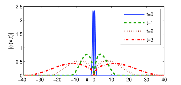
Figure 5. Profiles of the dispersive wave $|\phi(x,t)|$ at different $t$.

$$\begin{array}[]{cc}\psfig{height=136.5733pt,width=179.25244pt}&\psfig{height=136.5733pt,width=179.25244pt}\\ \psfig{height=136.5733pt,width=179.25244pt}&\psfig{height=136.5733pt,width=179.25244pt}\end{array}$$

Figure 6. Solution of the NLS $|\Phi(x,t)|$ and the soliton $\psi_{E(t)}(x)$ at different $t$.

Based on Figs. 4-6, we can draw the following observations:

1. The collective coordinates $E(t)$ and $\gamma(t)$ converge to the steady state as $t$ goes to infinity (cf. Fig. 4), and the dispersive part $\phi(x,t)$ spreads out to far field (cf. Fig. 5). The numerical results match with theoretical results in [26] very well.

2. The function $E(t)$ is not monotone in time $t$ (cf. the left figure in Fig. 4). This indicates that the process of the dynamics of the soliton and the dispersive wave is not monotone.

3. The dispersive wave $\phi$ in this case has a large expanding velocity (cf. Fig. 5). It is because that the chosen initial perturbation, i.e. the $\phi_{0}$ in (4.4), has a large $H^{1}$-norm. For the kind of situation, we remark that using the absorbing boundary conditions could be a more efficient way of study, which will be done in future consequential work.

4. For small time, the radiation term makes a big difference between the solution of NLS and the soliton (cf. Fig. 6). Thus, approximating the multichannel solution by the collective coordinates method in this example will call for a significant radiation correction. For large time, as the waves get close to the boundary of the computational domain, traditional numerical methods working the NLS cannot tell the soliton from the dispersive wave, while our approach of the modulation equations distinguish them exactly from the beginning.

Comparisons with classical numerical solver

To further show the advantages of modulation equations approach over classical numerical methods, we shorten the chosen computational domain to $\Omega=[-20,20]$, such that for time $t\geq 2$, the outgoing dispersive waves already reach the boundaries and are reflected back by the zero boundary conditions. Again we solve the NLS via the modulation equations approach with the SISP method with small time step and mesh size till $t=4$. As comparisons, we also solve the NLS directly with classical numerical method like the time-splitting sine spectral method or the finite difference time domain methods. Fig. 7 shows the numerical solutions of the NLS $|\Phi(x,t)|$ from the classical solver and the dispersive wave $|\phi(x,t)|$ from the modulation equations method at different $t$ after reflections happen. To check the influence bring by the reflected dispersive waves to the collective coordinates in our modulation approach, we compare the numerical values of $E(t)$ and $\gamma(t)$ obtained from the modulation equations method with the accurate values from Fig. 4. The errors at different $t$ are shown in Tab. 5. Based on Tab. 5 and Fig. 7, we can see: Both the numerical solution of the NLS from the classical solver and the numerical solution of the dispersive wave from modulation equations method are destroyed by the reflections in the computational domain compared to the exact solutions from Fig. 6. However in modulation equations approach, the error caused by the reflections to $E(t)$ and $\gamma(t)$ is always small during the computation. That is to say the small computational domain and the imposed boundary conditions will only break the dispersive part of the solution, but will hardly affect the soliton. The observation also give some clues to believe that using an absorbing boundary condition to the dispersive wave in (4.1a) could offer better results. While in classical numerical solvers, reflections will break both the soliton part and the dispersive part in the solution. Again we note that applying absorbing boundaries directly to the NLS will drag out the solitons as well [30]. Thus, to isolate the solitons from some initial matter waves in physical applications as BEC or optical lattice [6, 26], classical solvers need to choose a large computational domain and simulate for large time which is quite expensive in computational cost, while our approach do not.

Table 5. Error in collective coordinates $E(t)$ and $\gamma(t)$ caused by the reflections of the dispersive wave at the boundaries on domain $\Omega=[-20,20]$.

  $t=2$ $t=3$ $t=4$ $|e_{E}|$ 5.88E-05 5.92E-05 6.56E-05 $|e_{\gamma}|$ 1.00E-03 1.00E-03 4.29E-04  

$$\begin{array}[]{cc}\psfig{height=136.5733pt,width=179.25244pt}&\psfig{height=136.5733pt,width=179.25244pt}\\ \psfig{height=136.5733pt,width=179.25244pt}&\psfig{height=136.5733pt,width=179.25244pt}\\ \psfig{height=136.5733pt,width=179.25244pt}&\psfig{height=136.5733pt,width=179.25244pt}\end{array}$$

Figure 7. Numerical solutions of the NLS $|\Phi(x,t)|$ from classical solver and the dispersive wave $|\phi(x,t)|$ from modulation equations method on domain $\Omega=[-20,20]$ at different $t$.

Comparisons with collective coordinates method

In the last but not least comparison, we apply the collective coordinates method to study the multichannel solution via solving the model NLS problem

(5.1a) $$i\partial_{t}\Phi(x,t)=\left[-\partial_{xx}+V(x)+\lambda|\Phi|^{2}\right]\Phi(x,t),\quad x\in\mathbb{R},\ t>0,$$

(5.1b) $$\Phi(x,0)=\mathrm{e}^{i\gamma_{0}}\psi_{E_{0}}(x)+\phi_{0}(x),\quad x\in\mathbb{R},$$

where the potential, initial data, parameters are chosen same as (4.3) and (4.4), and the initial radiation

$$\phi_{0}(x)=\mathrm{e}^{i\alpha_{0}-B_{0}x}A_{0}x,\quad\mbox{with}\quad\alpha_{0}=-0.5,\ B_{0}=0.1,\ A_{0}=0.66.$$

The above model NLS is associated with the Lagrangian density

$$\mathcal{L}:=\frac{i}{2}(\Psi\overline{\Psi}_{t}-\overline{\Psi}\Psi_{t})+|\Psi_{x}|^{2}+V(x)|\Psi|^{2}+\frac{\lambda}{2}|\Psi|^{4},$$

and the averaged Lagrangian $L:=\int_{\mathbb{R}}\mathcal{L}dx$. As usually used in the literatures [1, 3, 5, 6, 11, 20, 24] and in particular [16, 23] where special attention has been paid to the interaction of solitons and radiation, the collective coordinates method takes the ansatz

(5.2) $$\Psi(x,t)=\mathrm{e}^{-i\theta(t)}\psi_{E(t)}(x)+\mathrm{e}^{i\alpha(t)}A(t)x\mathrm{e}^{-B(t)x^{2}},\quad x\in\mathbb{R},\ t>0,$$

with $\psi_{E(t)}$ the nonlinear bound state and five real-valued time dependent parameters $\theta(t)$, $E(t)$, $\alpha(t)$, $B(t)$ and $A(t)$. Plugging (5.2) into the Lagrangian $L$ and noting

$$E\int\psi_{E}^{2}dx=\int[(\partial_{x}\psi_{E})^{2}+V\psi_{E}^{2}+\lambda\psi_{E}^{4}]dx,$$

we get

(5.3) $$L= (-\dot{\theta}+E)\int_{\mathbb{R}}\psi_{E}^{2}dx-\frac{\lambda}{2}\int_{\mathbb{R}}\psi_{E}^{4}dx+A^{2}\int_{\mathbb{R}}(V+\dot{\alpha})x^{2}\mathrm{e}^{-2Bx^{2}}dx$$

$$+A^{2}\int_{\mathbb{R}}(1-2Bx^{2})^{2}\mathrm{e}^{-2Bx^{2}}dx+\frac{\lambda}{2}A^{4}\int_{\mathbb{R}}x^{4}\mathrm{e}^{-4Bx^{2}}dx$$

$$+\lambda A^{2}[1+2\cos^{2}(\theta+\alpha)]\int_{\mathbb{R}}x^{2}\psi_{E}^{2}\mathrm{e}^{-2Bx^{2}}dx.$$

Then by the Euler-Lagrangian equations from the variational principle, we get

(5.4a) $$\dot{\theta}=E+\lambda A^{2}[1+2\cos^{2}(\theta+\alpha)]\frac{\int_{\mathbb{R}}x^{2}\psi_{E}\partial_{E}\psi_{E}\mathrm{e}^{-2Bx^{2}}dx}{\int_{\mathbb{R}}\psi_{E}\partial_{E}\psi_{E}dx},\quad t>0,$$

(5.4b) $$\dot{E}=\lambda A^{2}\sin(2(\theta+\alpha))\frac{\int_{\mathbb{R}}x^{2}\psi_{E}^{2}\mathrm{e}^{-2Bx^{2}}dx}{\int_{\mathbb{R}}\psi_{E}\partial_{E}\psi_{E}dx},$$

$$\dot{\alpha}=-\frac{3\lambda A^{2}}{4B}-3B-\frac{4\sqrt{2}}{\sqrt{\pi}}\lambda B^{\frac{3}{2}}[1+2\cos^{2}(\theta+\alpha)]\int_{\mathbb{R}}x^{2}\psi_{E}^{2}\mathrm{e}^{-2Bx^{2}}dx$$

(5.4c) $$\quad\ \ \,-\frac{4\sqrt{2}}{\sqrt{\pi}}B^{\frac{3}{2}}\int_{\mathbb{R}}Vx^{2}\mathrm{e}^{-2Bx^{2}}dx,$$

(5.4d) $$\frac{\sqrt{\pi}}{4\sqrt{2}}B^{-\frac{3}{2}}\dot{A}-\frac{3\sqrt{\pi}}{16\sqrt{2}}B^{-\frac{5}{2}}A\dot{B}=-\lambda A\sin(2(\theta+\alpha))\int_{\mathbb{R}}x^{2}\psi_{E}^{2}\mathrm{e}^{-2Bx^{2}}dx,$$

$$\lambda c_{0}A^{2}=\frac{3\sqrt{\pi}}{4\sqrt{2}}B^{2}+B^{\frac{7}{2}}\int_{\mathbb{R}}V\mathrm{e}^{-2Bx^{2}}\left(x^{4}-\frac{3}{4B}x^{2}\right)dx$$

(5.4e) $$\qquad\quad\ +\lambda B^{\frac{7}{2}}[1+2\cos^{2}(\theta+\alpha)]\int_{\mathbb{R}}\psi_{E}^{2}\mathrm{e}^{-2Bx^{2}}\left(x^{4}-\frac{3}{4B}x^{2}\right)dx,$$

where $c_{0}=\left(\frac{9}{64\sqrt{2}}-\frac{15}{1024}\right)\sqrt{\pi}$, with initial data

$$A(0)=A_{0},\quad B(0)=B_{0},\quad\alpha(0)=\alpha_{0},\quad E(0)=E_{0},\quad\theta(0)=-\gamma_{0}.$$

Solving the above differential equations, we get the dynamics of the parameters predicted by the collective coordinates method. Fig. 8 shows the results related to the soliton, i.e. $E$ and $\theta$, together with comparisons with the results given by the modulation equation method, and Fig. 9 shows the radiation part.

$$\begin{array}[]{cc}\psfig{height=136.5733pt,width=179.25244pt}&\psfig{height=136.5733pt,width=179.25244pt}\\ \psfig{height=136.5733pt,width=179.25244pt}&\psfig{height=136.5733pt,width=179.25244pt}\end{array}$$

Figure 8. Left column: dynamics of the $E_{me}(t),\theta_{me}(t)$ given by modulation equation method and the $E_{cc}(t),\theta_{cc}(t)$ given by collective coordinates method in the comparison example (5.1). Right column: difference $|E_{me}(t)-E_{cc}(t)|$ and $|\theta_{me}(t)-\theta_{cc}(t)|$ between the two methods.

$$\begin{array}[]{cc}\psfig{height=136.5733pt,width=179.25244pt}&\psfig{height=136.5733pt,width=179.25244pt}\\ \psfig{height=136.5733pt,width=179.25244pt}&\psfig{height=136.5733pt,width=179.25244pt}\\ \psfig{height=136.5733pt,width=179.25244pt}&\psfig{height=136.5733pt,width=179.25244pt}\end{array}$$

Figure 9. The radiation $|\phi_{me}(x,t)|$ given by modulation equation method and the $|\phi_{cc}(x,t)|=A(t)\mathrm{e}^{-B(t)x^{2}}$ given by collective coordinates method at different $t$ in the comparison example (5.1). The last row shows the dynamics of the amplitude $A(t)$ and width $B(t)$ from the collective coordinates method.

From Figs. 8&9, we can see that: the predications given by the collective coordinates methods by using ansatz (5.2) are close to the exact solution in short time, especially in the soliton part. As time grows, the error from the predication tends to increases. This is mainly caused by the poor predication in the radiation at large time. As one can see in the last row of Fig. 9, the predicated radiation turns to move periodically which is not correct. The error from the radiation part will finally break the soliton and stop us from reaching the steady state. In fact unlike solitons, it is hard to capture the pattern of the radiation by finitely many variables in the collective coordinates method. In contrast, the modulation equation approach treats the radiation term exactly.

References

• [1] J. H. Al-Alawi: Collective coordinate approach to the dynamics of various soliton-obstruction systems. arXiv:0911.1804 [hep-th] (2009)
• [2] S. M. Alamoudi, U. Al Khawaja and B. B. Baizakov: Averaged dynamics of soliton molecules in dispersion-managed optical fibers. Phys. Rev. A, 89, pp. 053817 (2014)
• [3] S. M. Alamoudi, D. Boyanovsky and F. I. Takakura: Real-time dynamics of soliton diffusion. Phys. Rev. B, 57, pp. 919 (1998)
• [4] W. H. Aschbacher, J. Fröhlich, G. M. Graf, K. Schnee and M. Troyer: Symmetry breaking regime in the nonlinear Hartree equation. J. Math. Phys. 43, 3879 (2002)
• [5] H. E. Baron, G. Luchini and W. J. Zakrzewski: Collective coordinate approximation to the scattering of solitons in the (1+1) dimensional NLS model. J. Phys. A: Math. Theor., 47 pp. 265201 (2014)
• [6] A. Benseghir, W. A. T. Wan Abdullah, B. B. Baizakov and F. Kh. Abdullaev: Matter wave soliton bouncer. arXiv:1406.677v1 [cond-mat.quant-gas] (2014)
• [7] W. Bao and Y. Cai: Mathematical theory and numerical methods for Bose-Einstein condensation. Kinet. Relat. Models. 6, pp. 1–135 (2013)
• [8] W. Bao and Q. Du: Computing the ground state solution of Bose-Einstein condensates by a normalized gradient flow. SIAM J. Sci. Comput. 25, pp. 1674–1697 (2004)
• [9] W. Bao, D. Jaksch and P. A. Markowich: Numerical solution of the Gross-Pitaevskii equation for Bose-Einstein condensation. J. Comput. Phys. 187, pp. 318–-342 (2003)
• [10] Z. Chen, M. Segev and D. N. Christodoulides: Optical spatial solitons: historical overview and recent advances. Rep. Prog. Phys. 75, 086401 (2012)
• [11] J. H. P. Dawes and H. Susanto: Variational approximation and the use of collective coordinates. Phys. Rev. E, 87, pp. 063202 (2013)
• [12] M. D. Feit, J. A. Fleck and A. Steiger: Solution of the Schrödinger equations by a spectral method. J. Compt. Phy. 47, pp. 412-433 (1982)
• [13] G. H. Golub and V. L. Charles: Matrix Computations (3rd ed.). Baltimore: Johns Hopkins (1996)
• [14] D. Gottlieb and S. Orszag: Numerical Analysis of Spectral Methods: Theory and Applications. Society for Industrial and Applied Mathematics, Philadelphi (1993)
• [15] K. Javidan: Analytical formulation for soliton-potential dynamics. Phys. Rev. E, 10, pp. 466071–466078 (2008)
• [16] D. J. Kaup and B. A. Malomed: Embedded solitons in Lagrangian and semi-Lagrangian systems. Phys. D, 184, pp. 153–161 (2003)
• [17] F. G. Mertens, L. Morales-Molina, A. R. Bishop, A. Sánchez and P. Müller: Optimization of soliton ratchets in inhomogeneous sine-Gordon systems. Phys. Rev. E, 74, pp. 066602 (2006)
• [18] L. Morales-Molina, F. G. Mertens and A. Sánchez: Ratchet behavior in nonlinear Klein-Gordon systems with pointlike inhomogeneities. Phys. Rev. E, 72, pp. 016612 (2005)
• [19] L. Morales-Molina, F. G. Mertens and A. Sánchez: Soliton ratchets out of point-like inhomogeneities. Eur. Phys. J. B, 37, p. 79 (2004)
• [20] L. Morales-Molina, N. R. Quintero, A. Sánchez and F. G. Mertens: Soliton ratchets in homogeneous nonlinear Klein-Gordon systems. Chaos 16, pp. 013117 (2006)
• [21] M. Nishida, Y. Furukawa, T. Fujii and Noriyuki Hatakenaka: Breather-breather interactions in sine-Gordon systems using collective coordinate approach. Phys. Rev. E, 80, pp. 036603 (2009)
• [22] N. R. Quintero, A. Sánchez and F. G. Mertens: Resonances in the dynamics of $\varphi^{4}$ kinks perturbed by ac forces. Phys. Rev. E, 62, pp. 5695 (2000)
• [23] M. Syafwan, H. Susanto, S. M. Cox, and B. A. Malomed: Variational approximations for traveling solitons in a discrete nonlinear Schrödinger equation. J. Phys. A: Math. Theor., 45, pp. 075207 (2012)
• [24] A. Sánchez and A. R. Bishop: Collective coordinates and length-scale competition in spatially inhomogeneous soliton-bearing equations. SIAM Rev., 40, pp. 579–-615 (2006)
• [25] A. Soffer: Soliton dynamics and scattering. Proceedings of the International Congress of Mathematicians, Madrid, Spain. 3, pp. 459–471 (2006)
• [26] A. Soffer and M. I. Weinstein: Multichannel Nonlinear scattering for nonintegrable equations. Commun. Math. Phys. 133, pp. 119–146 (1990)
• [27] A. Soffer and M. I. Weinstein: Resonances, radiation damping and instability in Hamiltonian nonlinear wave equations. Invent. Math. 136, pp. 9–74 (1999)
• [28] A. Soffer and M. I. Weinstein: Selection of the ground state in the nonlinear Schrödinger equation. Rev. Math. Phys. 16, pp. 977–1071 (2004)
• [29] A. Soffer and M. I. Weinstein: Theory of nonlinear dispersive waves and selection of the ground state. Phys. Rev. Lett. 95, 213905 (2005)
• [30] A. Soffer and C. Stucchio: Open Boundaries for the Nonlinear Schrödinger Equation. J. Comp. Physics. 225, pp. 1218–1262 (2007)
• [31] J. Shen, T. Tang and L. Wang: Spectral Methods: algorithms, analysis and applications. Springer-Verlag, Berlin Heidelberg (2011)
• [32] H. Weigel: Kink-Antikink Scattering in $\psi^{4}$ and $\phi^{6}$ Models. arXiv:1309.6607 [nlin.PS] (2013)
• [33] E. Zamora-Sillero and A. V. Shapovalov: Equivalent Lagrangian densities and invariant collective coordinates equations. J. Phys. A: Math. Theor. 44, pp. 065204 (2011)