Quantum Dephasing of Interacting Quantum Dot Induced by the Superconducting Proximity Effect

Abstract

The proximity effect (PE) between superconductor and confined electrons can induce the effective pairing phenomena of electrons in nanowire or quantum dot (QD). Through interpreting the PE as an exchange of virtually quasi-excitation in a largely gapped superconductor, we found that there exists another induced dynamic process. Unlike the effective pairing that mixes the QD electron states coherently, this extra process leads to dephasing of the QD. In a case study, the dephasing time is inversely proportional to the Coulomb interaction strength between two electrons in the QD. Further theoretical investigations imply that this dephasing effect can decrease the quality of the zero temperature mesoscopic electron transportation measurements by lowering and broadening the corresponding differential conductance peaks.

I Introduction

Superconducting proximity effect (PE) was originally explored in the study of the normal-superconductor metals interface First proximity paper . When a sub-gap electron was injected from the normal side to a highly transparent interface, the Andreev reflection can happen, such that a hole is retro-reflected out from the superconducting side Andreev 1 ; Andreev 2 . This process is energy-favorable because Cooper pairs condense in the BCS ground state. As a result the extra electron pairs injected from the normal side can be absorbed without perturbing the superconductor.

Owing to the fast development in nanofabrication technology, novel effects in physics and related phenomena that discovered in hybrid devices have attracted much research interests especially in the searching for Majorana Fermions. Many previous investigations had taken the advantages of PE in producing exotic superconductivity with a p-wave component PE proposal 1 ; PE proposal 2 ; PE proposal 3 ; PE proposal 4 . In those proposals, usually a nanowire with strong spin-orbit coupling is placed in close contact with a bulk s-wave pairing superconductor (SC), such that electron can tunnel between SC and the nanowire. If one focus on physics inside the SC gap, an effective Hamiltonian for the nanowire can be derived with additional terms describing electron pair creation or annihilation Proximity induced pairing 1 ; Proximity induced pairing 2 , which are referred as PE induced pairing terms. Although those proposals stimulate a series of experimental works with significant results nanowire experiment 1 ; nanowire experiment 2 ; nanowire experiment 3 , the nanowire-based setup has its drawbacks such as difficulties in manipulating chemical potential nanowire experiment 1 ; QD chain 1 as well as fragile of the induced pairing potential against disorder QD chain 2 .

To overcome those obstacles, analogy in other systems Other modified nanowire prop. or modified solid-system proposals have been suggested. A notable trend among those is to replace the nanowire by a chain of coupled quantum dots (QD), which is introduced by J. D. Sau et al in ref. QD chain 1 and further developed by many groups QD chain 2 ; QD chain 4 ; QD chain 3 ; QD chain 5 . However, many discussions in this aspect adopt directly the discretized version of the previous effective Hamiltonians of the nanowire that are obtained based on the single electron picture. Meanwhile, in QD related transport studies, there are also researches which point out that a large Coulomb repulsion can suppress onsite PE pairing Coulomb int kill PE 1 ; single-level anderson 1 , and the above is actually the key idea of the Cooper pair beam splitter Proximity induced pairing 2 . Those observations motivated us to investigate whether interaction effect can be important or not in discussing PE on the QD.

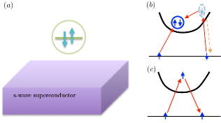
Figure 1: (Color online) (a) Schematic plot of a single level quantum dot (QD) in proximity to a bulk s-wave pairing superconductor (SC). (b) Pictorial representation of the Andreev reflection, where the black parabolic curve denotes the quasi-excitation state of the SC and the horizontal line at the bottom denotes energy of the QD level. (c) Pictorial illustration on virtual process that is relevant for the proximity induced dephasing effect.

In this paper, we present a theoretical approach that can be used to explore PE on the QD system when the onsite Coulomb interaction strength was much smaller than the SC gap. The idea is based on adiabatic eliminating the SC quasi-excitation, since the electron tunneling between QD and SC becomes virtual due to the large SC gap. Then, we apply this approach to a simplified model with only one QD. The corresponding effective Hamiltonian of QD reduces to previous ones if the Coulomb interaction is ignored. However, when the Coulomb interaction was included, new terms representing interactions between QD and SC are identified besides the previously obtained pairing terms. To the leading order, the main contribution comes from a dephasing term that can force the QD to evolve into a mixed state.

This paper is organized as follows, in Sec. II we bring in the QD model and use the adiabatic elimination scheme to derive the effective Hamiltonian of QD. In Sec. III, the decoherence factor as well as the dephasing time of QD are evaluated by employing a semi-classical treatment. Physical implication of the PE induced dephasing is discussed in Sec. IV by studying the transport properties of QD in a three-terminals quantum point contact device. Finally a summary is given in Sec. V.

II Adiabatic elimination and proximity induced dephasing

Let us consider a QD which is located near a bulk SC, as schematically shown in Fig.1(a). For simplicity consideration we model the QD as a single band Anderson impurity single-level anderson 1 ; single-level anderson 2 ; single-level anderson 3 , although generalization to the cases of finite size non-Anderson impurtity for QD ; non-Anderson impurtity for QD 2 as well as multiple levels multi-level QD 1 ; multi-level QD 2 are possible. The SC is described by an s-wave pairing mean-field BCS Hamiltonian with real pairing potential $\Delta$. Consequently, Hamiltonian of the QD-SC hybrid system is written as $H=H_{d}+H_{s}+H_{sd},$ with

$$H_{d}=\varepsilon\sum_{\sigma}n_{\sigma}+Un_{\uparrow}n_{\downarrow},$$ (1)

$$H_{s}=\sum_{\mathbf{k}}[\xi_{\mathbf{k}}(c_{k}^{\dagger}c_{k}+c_{-k}^{\dagger}c_{-k})+\Delta(c_{k}^{\dagger}c_{-k}^{\dagger}+c_{-k}c_{k})],$$ (2)

and

$$H_{sd}=\sum_{\mathbf{k},\sigma}(t_{\mathbf{k}}d_{\sigma}^{\dagger}c_{\mathbf{k}\sigma}+h.c.).$$ (3)

Here, $H_{d}$ and $H_{s}$ are the Hamiltonians of the QD and the SC, respectively. $n_{\sigma}=d_{\sigma}^{\dagger}d_{\sigma}$ is QD electron number operator with electron spin $\sigma\in\{\uparrow,\downarrow\}$. $\varepsilon=\epsilon_{d}-\mu$ is energy of the QD level measured from the chemical potential $\mu$ of the SC, $U$ is the onsite Coulomb interaction strength for double occupation of the QD. $\xi_{\mathbf{k}}=\mathbf{k}^{2}/(2m)-\mu$ is the kinetic energy of a free electron measured from $\mu$. We use $k=\{\mathbf{k},\uparrow\}$ and $-k=\{-\mathbf{k},\downarrow\}$ to jointly label momentum and spin for the SC electrons. $H_{sd}$ describes the single electron tunneling process. For tunneling that happens locally in space, as relevant to quantum point contact (QPC), the corresponding tunneling probability amplitude $t_{\mathbf{k}}=t_{0}\exp\{i\mathbf{k}\cdot\vec{r}\}$. Here $t_{0}$ is assumed to be real and $\vec{r}$ denotes the location of QD.

$H_{s}$ can be diagonalized by the following Bogoliubov transformation

$$\gamma_{k}=\cos\theta_{k}c_{k}+\sin\theta_{k}c_{-k}^{\dagger},\mbox{ }\gamma_{-k}=\cos\theta_{k}c_{-k}-\sin\theta_{k}c_{k}^{\dagger},$$ (4)

where $\tan 2\theta_{k}=\Delta/\xi_{\mathbf{k}}$ and notice that $\{\gamma_{k},\gamma_{-k^{\prime}}^{\dagger}\}=0$. After the Bogoliubov transformation, $H_{s}$ is rewritten as

$$H_{s}=\sum_{\mathbf{k}}E_{\mathbf{k}}(\gamma_{k}^{\dagger}\gamma_{k}+\gamma_{-k}^{\dagger}\gamma_{-k}),$$ (5)

where $E_{\mathbf{k}}=\sqrt{\xi_{\mathbf{k}}^{2}+\Delta^{2}}$ is the elementary excitation spectrum of the SC. $H_{sd}$ is also rewritten as follows in terms of quasi-particle operators $\gamma_{k}$ and $\gamma_{-k}$, i.e.,

$$H_{sd}=\sum_{\mathbf{k}}[\eta_{\mathbf{k}}(d_{\uparrow}^{\dagger}\gamma_{k}-d_{\downarrow}\gamma_{-k}^{\dagger})-\lambda_{\mathbf{k}}(d_{\downarrow}\gamma_{k}+d_{\uparrow}^{\dagger}\gamma_{-k}^{\dagger})+h.c.].$$ (6)

In the sub-gap regime (SGR), i.e., both $U\ll\Delta$ and $\varepsilon\ll\Delta$, all relevant QD states are within the SC gap. Thus the minimal energy gap between electron states in the QD and quasi-excitation states in the SC is $\delta\omega=\min\{\left|\Delta-\varepsilon\right|,\left|\Delta-\varepsilon-U\right|\}$. Suppose that the tunneling strength between SC and QD further satisfies $t_{0}/\delta\omega\ll 1$, then one can eliminated $H_{sd}$ up to the first order by performing the canonical transformation $\exp(S)$ Adiabatic elimination 1 ; Adiabatic elimination 2 , where

$$S=\sum_{\mathbf{k}}[\alpha_{\mathbf{k}}(D_{\uparrow}^{\dagger}\gamma_{k}+D_{\downarrow}\gamma_{-k}^{\dagger})-\beta_{\mathbf{k}}(\tilde{D}_{\downarrow}\gamma_{k}-\tilde{D}_{\uparrow}^{\dagger}\gamma_{-k}^{\dagger})-h.c.].$$ (7)

Here, $\alpha_{\mathbf{k}}$, $\beta_{\mathbf{k}}$, $D_{\sigma}$ and $\tilde{D}_{\sigma}$ are

$$\alpha_{\mathbf{k}}=\frac{\eta_{\mathbf{k}}}{E_{\mathbf{k}}-\varepsilon},\mbox{ }\beta_{\mathbf{k}}=\frac{\lambda_{\mathbf{k}}}{E_{\mathbf{k}}+\varepsilon},$$ (8)

and

$$D_{\sigma}=d_{\sigma}(1+\frac{Un_{\bar{\sigma}}}{E_{\mathbf{k}}-\varepsilon-U}),\mbox{ }\tilde{D}_{\sigma}=d_{\sigma}(1-\frac{Un_{\bar{\sigma}}}{E_{\mathbf{k}}+\varepsilon+U}).$$ (9)

Here, $\eta_{\mathbf{k}}=t_{\mathbf{k}}\cos\theta_{k}$ and $\lambda_{\mathbf{k}}=t_{\mathbf{k}}\sin\theta_{k}$. $\bar{\sigma}$ denotes the spin direction opposite to $\sigma$.

After the canonical transformation, Hamiltonian of the hybrid system is written as

$$e^{-S}He^{S}\approx H_{d}^{\mathrm{eff}}+H_{s}^{\mathrm{eff}}+H_{sd}^{\mathrm{eff}},$$ (10)

where $H_{d}^{\mathrm{eff}}$ is given by

$$H_{d}^{\mathrm{eff}}=H_{d}+(\Delta_{d}d_{\uparrow}^{\dagger}d_{\downarrow}^{\dagger}+h.c.),$$ (11)

$\Delta_{d}$ is PE induced pairing potential in the QD,

$$\Delta_{d}=t_{0}^{2}\sum_{\mathbf{k}}\frac{\Delta}{E_{\mathbf{k}}^{2}-\varepsilon^{2}}=\frac{\pi t_{0}^{2}N_{0}\Delta}{\sqrt{\Delta^{2}-\varepsilon^{2}}}.$$ (12)

Here, $N_{0}$ is normal state density of state (DOS) at $\mu$. Eq.(12) has been obtained before in weak tunneling limit PE induced pairing in waek tunneling 1 ; Proximity induced pairing 1 . Notice that $\Delta_{d}$ saturates to a constant value that independent from $\Delta$ in the SGR.

Notice that generally all parameters involved in $H_{d}$ of Eq.(11) should be renormalized when compared with parameters defined in Eq.(1), but in the following we shall not distinguish this difference and still adopt the previous notations for an isolated QD. Furthermore, we take $H_{s}^{\mathrm{eff}}\approx H_{s}$ since the back action of the QD on the SC should be minor.

$H_{sd}^{\mathrm{eff}}$ denotes interactions between QD and SC, full expression of this term is given in the Appendix A. By averaging $H_{sd}^{\mathrm{eff}}$ over the BCS ground state of the SC, the only contributing term has the following form

$$H_{sd}^{\mathrm{eff}}\approx\sum_{\sigma}n_{\sigma}\otimes R_{\sigma},$$ (13)

where $R_{\sigma}$ are two operators acting only on Hilbert space of the SC, i.e.,

$$R_{\uparrow} = \frac{1}{2}\sum_{\mathbf{k},\mathbf{k}^{\prime}}[\tilde{\alpha}_{\mathbf{k}^{\prime}}(\eta_{\mathbf{k}}^{*}\eta_{\mathbf{k}^{\prime}}\gamma_{-k^{\prime}}^{\dagger}\gamma_{-k}-\lambda_{\mathbf{k}}^{*}\eta_{\mathbf{k}^{\prime}}\gamma_{k}^{\dagger}\gamma_{-k^{\prime}}^{\dagger})$$ (14)

$$+\tilde{\beta}_{\mathbf{k}^{\prime}}(\lambda_{\mathbf{k}}^{*}\lambda_{\mathbf{k}^{\prime}}\gamma_{k^{\prime}}\gamma_{k}^{\dagger}+\eta_{\mathbf{k}}^{*}\lambda_{\mathbf{k}^{\prime}}\gamma_{k^{\prime}}\gamma_{-k})+h.c.],$$

and

$$R_{\downarrow} = \frac{1}{2}\sum_{\mathbf{k},\mathbf{k}^{\prime}}[-\tilde{\beta}_{\mathbf{k}^{\prime}}(\lambda_{\mathbf{k}}^{*}\lambda_{\mathbf{k}^{\prime}}\gamma_{-k}\gamma_{-k^{\prime}}^{\dagger}+\eta_{\mathbf{k}}^{*}\lambda_{\mathbf{k}^{\prime}}\gamma_{-k^{\prime}}^{\dagger}\gamma_{k}^{\dagger})$$ (15)

$$+\tilde{\alpha}_{\mathbf{k}^{\prime}}(\eta_{\mathbf{k}}^{*}\eta_{\mathbf{k}^{\prime}}\gamma_{k}^{\dagger}\gamma_{k^{\prime}}-\lambda_{\mathbf{k}}^{*}\eta_{\mathbf{k}^{\prime}}\gamma_{-k}\gamma_{k^{\prime}})+h.c.],$$

where

$$\tilde{\alpha}_{\mathbf{k}}=\frac{U}{(E_{\mathbf{k}}-\varepsilon)(E_{\mathbf{k}}-\varepsilon-U)},\mbox{ }\tilde{\beta}_{\mathbf{k}}=\frac{U}{(E_{\mathbf{k}}+\varepsilon)(E_{\mathbf{k}}+\varepsilon+U)}.$$ (16)

Notice that both $\tilde{\alpha}_{\mathbf{k}}$ and $\tilde{\beta}_{\mathbf{k}}$ approach to zero as $U$ goes to zero, thus indicating the Coulomb interaction is necessary in producing coupling term given by Eq.(13).

A basis for the QD is chosen as $\{|0\rangle,|\sigma\rangle,|d\rangle\}$, where $|0\rangle$ and $|d\rangle$ denote the emptily as well as the doubly occupied state of the QD, and $|\sigma\rangle$ are single occupation states with spin $\sigma$. It follows from Eq.(11) that the PE induced pairing term causes mixing of basis states in the subspace spanned by $|0\rangle$ and $|d\rangle$, while the single electron subspace $\{|\sigma\rangle\}$ remains unaffected by this term. However, the quantum coherence between spin-up and spin-down states in the latter subspace can still lose due to coupling with the SC through the term $H_{sd}^{\mathrm{eff}}$. This is because, with the additional term $H_{sd}^{\mathrm{eff}}$, the superconductor now can evolve differently depending on spin orientation of the QD electron. This PE induced dephasing (PID) effect would be absent if one ignores the onsite Coulomb interaction.

III the dephasing time

The PID process and subsequent decoherence of the QD deserve more detailed investigation, since quantum coherence is a crucial resource in implementing various quantum computations quantum coherence 1 ; quantum coherence 2 . To this end, we estimate characteristic dephasing time of the QD by studying its decoherence factor.

Since the single electron subspace is decoupled from the subspace $\{|0\rangle,|d\rangle\}$, we shall restrict following discussion only to the case of single electron. Consider following initial state for the hybrid system with one electron in the QD

$$|\Phi(0)\rangle=\sum_{\sigma}w_{\sigma}|\sigma\rangle\otimes|BCS\rangle,$$ (17)

where $|w_{\sigma}|^{2}$ is probability for electron to occupy the state $|\sigma\rangle$. $|BCS\rangle$ denotes the BCS ground state of the SC. After a period of evolution, the final state becomes

$$|\Phi(t)\rangle=\sum_{\sigma}w_{\sigma}e^{-is[\sigma]\varepsilon t}|\sigma\rangle\otimes e^{-ih_{\sigma}t}|BCS\rangle.$$ (18)

Here, $s[\uparrow]=1$ and $s[\downarrow]=-1$. $h_{\sigma}$ is defined as $h_{\sigma}=H_{s}+R_{\sigma}$.

To discuss the QD dephasing, we consider the reduced density matrix of the QD system. This is given by

$$\rho(t) = \mbox{tr}_{\mathrm{sc}}\{|\Phi(t)\rangle\langle\Phi(t)|\}$$ (19)

$$= |c_{\uparrow}|^{2}|\uparrow\rangle\langle\uparrow|+|c_{\downarrow}|^{2}|\downarrow\rangle\langle\downarrow|$$

$$+(c_{\uparrow}c_{\downarrow}^{*}e^{-2i\varepsilon t}|\uparrow\rangle\langle\downarrow|D(t)+h.c.).$$

Here, $\mathrm{tr}_{\mathrm{sc}}$ means tracing over the degree of freedom of the SC. $D(t)$ is the decoherence factor of QDdecoherence factor ,

$$D(t)=\langle e^{ih_{\downarrow}t}e^{-ih_{\uparrow}t}\rangle_{\mathrm{sc}},$$ (20)

where the averaging is taken with respect to $|BCS\rangle$.

Since $h_{\sigma}$ is quadratic in quasi-particle operators, the exact evaluation of $D(t)$ is always possible but too complicated to be done. Therefore, we adopt a semi-classical treatment to estimate $D(t)$. We remark that this method is equivalent to second order cumulant expansion second order cum if sum over $\mathbf{k}\neq\mathbf{k}^{\prime}$ terms involved in $R_{\sigma}$ are ignored. The idea of this semi-classical method is to replace $R_{\sigma}$ by a random number $\mathcal{R}_{\sigma}$, whose mean value and covariance are determined quantum mechanically by using following relations

$$\langle\mathcal{R}_{\sigma}\rangle_{\mathrm{cl}}=\langle R_{\sigma}\rangle_{\mathrm{sc}},\mbox{ }\langle\langle\mathcal{R}_{\sigma}\mathcal{R}_{\sigma^{\prime}}\rangle\rangle_{\mathrm{cl}}=\langle R_{\sigma}R_{\sigma^{\prime}}\rangle_{\mathrm{sc}}-\langle R_{\sigma}\rangle_{\mathrm{sc}}\langle R_{\sigma^{\prime}}\rangle_{\mathrm{sc}},$$ (21)

Also the quantum mechanically trace in $D(t)$ is replaced by averaging over probability density function (PDF) of $\mathcal{R}_{\sigma}$.

In this way, $D(t)$ is rewritten as

$$D(t)\approx\langle e^{-i(\mathcal{R}_{\uparrow}-\mathcal{R}_{\downarrow})t}\rangle_{\mathrm{cl}}.$$ (22)

Using the following cumulant expansion formula Van Kampen book

$$\langle e^{\alpha\delta x+\beta\delta y}\rangle_{\mathrm{cl}}$$

$$\approx e^{\alpha\langle\delta x\rangle_{\mathrm{cl}}+\beta\langle\delta y\rangle_{\mathrm{cl}}+\frac{1}{2}\alpha^{2}\langle\langle\delta x^{2}\rangle\rangle_{\mathrm{cl}}+\frac{1}{2}\beta^{2}\langle\langle\delta y^{2}\rangle\rangle_{\mathrm{cl}}+\alpha\beta\langle\langle\delta x\delta y\rangle\rangle_{\mathrm{cl}}},$$

$D(t)$ is further expressed as

$$D(t)\approx e^{-i\Omega t}e^{-\Gamma^{2}t^{2}},$$ (24)

where

$$\Omega=2\langle\mathcal{R}_{\uparrow}\rangle_{\mathrm{cl}},\mbox{ }\Gamma=\sqrt{\frac{1}{2}\sum_{\sigma}\langle\langle\mathcal{R}_{\sigma}^{2}\rangle\rangle_{\mathrm{cl}}-\langle\langle\mathcal{R}_{\uparrow}\mathcal{R}_{\downarrow}\rangle\rangle_{\mathrm{cl}}}.$$ (25)

Notice that in deriving Eq.(25), we have used $\langle\mathcal{R}_{\sigma}+\mathcal{R}_{\bar{\sigma}}\rangle_{\mathrm{cl}}=0$. Proof of this relation can be found in Appendix B.

According to Eqs.(24,25), the dephasing time of QD is defined as $T_{\mathrm{ph}}=\Gamma^{-1}$. If QD energy is chosen such that $\varepsilon=-U/2$, then $T_{\mathrm{ph}}$ has the following analytical expression (see Appendix B), i.e.,

$$T_{\mathrm{ph}}=|\zeta(\Delta)|\frac{\Delta}{U\Delta_{d}},$$ (26)

where $\zeta^{2}(\Delta)=\pi\sqrt{(\Delta^{2}-U^{2}/4)/(\Lambda_{D}^{2}-\Delta^{2})}$ depends mainly on $\Delta$ since $U\ll\Delta$. $\Lambda_{D}$ is characteristic width of energy shell where the SC electron-electron effective attraction is non-zero. It follows from Eq.(12) that $\Delta_{d}$ is asymptotically independent from $\Delta$ in the SGR. Then $T_{\mathrm{ph}}$ is proportional to $\Delta$ and inversely proportional to the Coulomb interaction strength, which means that the dephasing effect becomes weaker as SC gap became larger or Coulomb interaction became smaller.

IV Observable effects of the proximity induced dephasing

The PID effect manifest itself as a quantum fluctuation on QD levels as a result of virtual quasi-particle exchanging with the SC. This modulation on the energy level can be probed by the measurement on mesoscopic transport through a QPC, which at low temperature provides the information about the local density of states at the QD STM prob local density state . Besides this, although it has been predicted that an observation of a quantized zero-bias peak in differential conductance measurement can be regarded as a necessary condition for the judgment on the existence of Majorana quasi-particles quantise ZBP theoretic , the experimental results on transport studies display peaks that are much lower than this theoretical prediction nanowire experiment 1 ; ZBP less then 2 e2/h . This fact has motivated several explorations on the possible explanations ZBP explain 1 ; ZBP explain 2 ; ZBP explain 3 , which also attract us to consider the PID effect on transport setups. In fact, there has been some transport based researches on the effect of dephasing caused by electron-electron interaction in QD systems QD dephasing ; QD dephasing 2 .

Let us consider a three terminals transport device with two leads in normal and one in the superconducting states, as schematically shown in Fig.2(a). Similar multi-terminals devices have been investigated in ref. QD dephasing ; multi-terminal 1 ; multi-terminal 2 . The Hamiltonian of the system is written as $H_{\mathrm{tot}}=H+\sum_{\nu=L,R}(H_{\nu}+H_{\nu d})$, with

$$H_{\nu}=\sum_{\mathbf{k},\sigma}\xi_{\mathbf{k}}c_{\nu\mathbf{k}\sigma}^{\dagger}c_{\nu\mathbf{k}\sigma},$$ (27)

and

$$H_{\nu d}=\sum_{\mathbf{k},\sigma}(t_{\mathbf{k}}^{(\nu)}d_{\sigma}^{\dagger}c_{\nu\mathbf{k}\sigma}+h.c.).\mbox{ }(\nu=L,R)$$ (28)

Here $H$ is given by Eqs.(1-3), which describes the SC lead, the QD, as well as single electron tunneling that happened between the two. $H_{\nu}$ is Hamiltonian of the normal lead $\nu$ with chemical potential $\mu_{\nu}$, notice that the kinetic energy is again measured from the SC chemical potential $\mu$. $H_{\nu d}$ denotes the electron tunneling between the QD and normal lead $\nu$. For the localized tunneling $t_{\mathbf{k}}^{(\nu)}=t_{\nu}\exp\{i\mathbf{k}\cdot\vec{r}\}$ and $t_{\nu}$ are assumed to be real.

Suppose that the pairing potential of the SC lead is chosen to satisfy the SGR conditions. Then according to the results in Sec. II, $H$ can be replaced by $H_{d}^{\mathrm{eff}}+H_{sd}^{\mathrm{eff}}$, i.e., the role of the SC lead is included effectively by using the adiabatic elimination approach. Therefore, in this case we can focus on the current through the QD between two normal leads. The current from lead $\nu$ is written as

$$I_{\nu} = \langle\frac{d}{dt}N_{\nu}\rangle=-ie\langle[H_{\mathrm{tot}},N_{\nu}]\rangle.$$ (29)

Here, $N_{\nu}=\sum_{\mathbf{k},\sigma}c_{\nu\mathbf{k}\sigma}^{\dagger}c_{\nu\mathbf{k}\sigma}$ is the total number of electrons in the lead $\nu$. In the Heisenberg picture, the above averaging is taken with respect to initial state of the whole system. Notice that the chemical potentials of two normal leads are not always the same due to applied bias voltage, as shown in Fig.2(b).

Figure 2: (Color online) (a) Schematic of a three-terminals device in quantum point contact (QPC) with a single level quantum dot (QD), one of those leads is in the BCS superconducting ground state (shown in purple). In the sub-gap regime (SGR), real single electron tunneling between QD and the superconducting (SC) lead does not happen, as stressed by dashed red arrows. (b) Energy landscape of the multi-terminals QPC system, where the bias voltage is applied between two normal leads. The QD level with energy $\varepsilon$ (measured from SC chemical potential $\mu$) is shown by green solid line inside the SC gap.

The total current through the QD is given by $I_{\mathrm{tot}}=(I_{L}-I_{R})/2$. In steady state, $I_{\mathrm{tot}}$ can be expressed in terms of Green’s function of the QD by using the non-equilibrium techniques Wingreen , i.e.,

$$I_{\mathrm{tot}}=-\frac{e\Gamma_{0}}{h}\sum_{\sigma}\int d\omega\mathrm{Im}[g_{\sigma}^{r}(\omega)][f_{L}(\omega+\mu)-f_{R}(\omega+\mu)],$$ (30)

where the Plank constant $h$ is written out explicitly. The above equation is valid in the width band limit Wingreen , where the DOS of the normal leads are assumed as constant within the energy spectrum of the single level QD. We also assumed that $t_{L}=t_{R}=t_{1}$, thus the line width function $\Gamma_{0}=2\pi t_{1}^{2}N_{0}$ is the same for both normal leads multi-level QD 1 . $f_{\nu}(\omega)$ is the equilibrium state Fermi-distribution at lead $\nu$, i.e., $f_{\nu}(\omega)=\{\exp[\beta(\omega-\mu_{\nu})]+1\}^{-1}$.

$g_{\sigma}^{r}(\omega)$ is Fourier transform of the retarded QD Green’s function,

$$g_{\sigma}^{r}(t,t^{\prime})=-i\theta(t-t^{\prime})\langle\{d_{\sigma}(t),d_{\sigma}^{\dagger}(t^{\prime})\}\rangle,$$ (31)

which is the key quantity in evaluating $I_{\mathrm{tot}}$.

At low temperature, the Fermi-distribution function can be approximated by the step-function, i.e., $f_{\nu}(\omega)\approx\theta(\mu_{\nu}-\omega)$. Suppose $\mu_{R}=\mu$, then $I_{\mathrm{tot}}$ is rewritten as

$$I_{\mathrm{tot}}=-\frac{e\Gamma_{0}}{h}\sum_{\sigma}\int_{0}^{eV}d\omega\mathrm{Im}g_{\sigma}^{r}(\omega),$$ (32)

where $V=(\mu_{L}-\mu_{R})/e$ denotes the bias voltage across two normal leads. Differential conductance is then given by

$$\frac{dI_{\mathrm{tot}}}{dV}=-\frac{e^{2}}{h}\Gamma_{0}\sum_{\sigma}\mathrm{Im}g_{\sigma}^{r}(eV).$$ (33)

According to the derivation detailed in Appendix C, at the mean-field level MF app 1 ; MF app 2 $g_{\sigma}^{r}(\omega)$ is calculated by using the motion equation method, i.e.,

$$g_{\sigma}^{r}(\omega)=\frac{D_{h}(\omega)G_{\sigma}^{(e)}(\omega)}{D_{e}(\omega)D_{h}(\omega)-\Delta_{d}^{2}G_{\bar{\sigma}}^{(e)}(\omega)G_{\sigma}^{(h)}(\omega)}$$ (34)

with

$$D_{e}(\omega)=\omega-\varepsilon-(\mathcal{R}_{\sigma}-i\Gamma_{0})G_{\sigma}^{(e)}(\omega),$$ (35)

$$D_{h}(\omega)=\omega+\varepsilon+(\mathcal{R}_{\bar{\sigma}}+i\Gamma_{0})G_{\bar{\sigma}}^{(h)}(\omega),$$ (36)

$$G_{\sigma}^{(e)}(\omega)=1+\frac{U\langle n_{\bar{\sigma}}\rangle_{0}}{\omega-\varepsilon-U+i0^{+}},$$ (37)

and

$$\mbox{ }G_{\sigma}^{(h)}(\omega)=1-\frac{U\langle n_{\bar{\sigma}}\rangle_{0}}{\omega+\varepsilon+U+i0^{+}}.$$ (38)

Notice that in obtaining the above results, the semi-classical treatment for the PID term introduced before in Sec. III had been used. Sub-index in $\langle n_{\sigma}\rangle_{0}$ indicates to take the atomic limit (AL) STM prob local density state , where $t_{0}$ and $t_{1}$ are set to zero in evaluating the averaging $\left\langle...\right\rangle_{0}$.

Due to the semi-classical treatment, Eq.(33) should be averaged over PDF of $\mathcal{R}_{\sigma}$,

$$\langle\frac{dI_{\mathrm{tot}}}{dV}\rangle_{\mathrm{cl}}=-\frac{e^{2}}{h}\Gamma_{0}\sum_{\sigma}\mathrm{Im}\langle g_{\sigma}^{r}(eV)\rangle_{\mathrm{cl}},$$ (39)

Notice that in writing $\langle\mathrm{Im}g_{\sigma}^{r}(eV)\rangle_{\mathrm{cl}}=\mathrm{Im}\langle g_{\sigma}^{r}(eV)\rangle_{\mathrm{cl}}$, we have implicitly assumed that there exists real PDF for $\mathcal{R}_{\sigma}$ that satisfy Eq.(21), but this point has not been explicitly checked.

To calculate differential conductance we need to evaluate $\langle g_{\sigma}^{r}(\omega)\rangle_{\mathrm{cl}}$. This can be done analytically in a special case where $\varepsilon=-U/2$ and $\langle n_{\sigma}\rangle_{0}=1/2$. As outlined in Appendix D, in this case the Green’s function can be evaluated by using a cumulant expansion method similar to that employed in Sec. III. The result is

$$\langle g_{\sigma}^{r}(\omega)\rangle_{\mathrm{cl}}$$

$$= \frac{\omega}{\omega^{2}-\varepsilon^{2}+q_{\sigma}^{(e)}(\omega)+i\Gamma_{\sigma}\omega-\frac{\Delta_{d}^{2}\omega^{2}}{\omega^{2}-\varepsilon^{2}+q_{\bar{\sigma}}^{(h)}(\omega)+i\Gamma_{\bar{\sigma}}\omega}}.$$

Here, $q_{\sigma}^{(e,h)}(\omega)$ depends on $\langle\mathcal{R}_{\sigma}\rangle_{\mathrm{cl}}$ and slightly shifts poles of $\langle g_{\sigma}^{r}(\omega)\rangle_{\mathrm{cl}}$, their expressions are given by Eqs.(D7,D8). $\Gamma_{\sigma}$ is related to differential conductance in the absence of the PID effect, i.e.,

$$\Gamma_{\sigma}=\Gamma_{0}+\frac{h}{2\Gamma_{0}e^{2}}\frac{dI_{\mathrm{tot}}}{dV}|_{\mathcal{R_{\sigma}}\equiv 0}\langle\langle\mathcal{R}_{\sigma}^{2}\rangle\rangle_{\mathrm{cl}}.$$ (41)

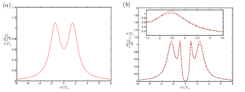
Figure 3: (Color online) Differential conductance calculated based on the semi-classical treatment, black dashed (red solid) line is result with (without) the proximity induced dephasing (PID) effect. We have set $\mu_{R}=\mu$ in those calculations, other parameters used are: $U/\Gamma_{0}=0\mbox{ and }3$ for (a) and (b), respectively; $\Gamma_{s}\equiv 2\pi t_{0}^{2}N_{0}=3\Gamma_{0}$, $\varepsilon=-U/2$, $\Delta/\Gamma_{0}=10$, $\Lambda_{D}/\Gamma_{0}=100$. With this choice of parameters, the PE induced pairing potential $\Delta_{d}\sim\Delta/7$.

Since the differential conductance is related to the imaginary part of the QD Green’s function, consequently $\Gamma_{\sigma}$ determines the width of conductance peaks. Therefore, the second term in Eq.(41) represents the PID effect on the peaks width. Notice that $(dI_{\mathrm{tot}}/dV)|_{\mathcal{R_{\sigma}}\equiv 0}$ is positive. This can be checked by setting $q_{\sigma}^{(e,h)}(\omega)=0$ and $\Gamma_{\sigma}=\Gamma_{0}$ in Eq.(LABEL:g_retard_semi-classical) followed by taking imaginary part. On the other hand, if $\Lambda_{D}\gg\Delta$, it follows from the results shown in the Appendix B (see Eqs.(B10-B13), for example) that $\langle\langle\mathcal{R}_{\sigma}^{2}\rangle\rangle_{\mathrm{cl}}$ are positive. As a result $\Gamma_{\sigma}\geq\Gamma_{0}$, this means that due to the PID effect, differential conductance measured at low temperature will become broader.

In Fig.3, differential conductance is calculated numerically by using Eq.(39). By making comparisons between the calculated results, the inclusion of the Coulomb interaction further splits the conductance peaks. This splitting is expectable, because the DOS of the QD is changed due to the electron-electron repulsion in case of double occupation. However, the calculation also revivals that all peaks become lower and slightly broaden when the PID effect was included.

In this section, one of the potential observable phenomena due to the PID effects is explored. We investigate the transport current through a multi-terminals QPC device. The PID effect enters into the problem since one of those terminals is assumed to satisfy the SGR condition, consequently its role is included effectively according to the adiabatic elimination approach presented in Sec.II. The steady state current is calculated by combining the non-equilibrium Green’s function method with the semi-classical approach outlined in Sec.III. The results show us that the height of differential conductance peaks decreases as a result of the PID effect. This phenomena is controlled by $\langle\langle\mathcal{R}_{\sigma}^{2}\rangle\rangle_{\mathrm{cl}}$, which are in turn related to parameters of the proximity coupling, e.g., $t_{0}$ and $\Delta$.

V Conclusion

To conclude, we present an adiabatic elimination approach to incorporate PE in SC-QD hybrid system. This method rely on the SGR condition, where all QD levels are located inside the SC gap. Apart from those already known PE induced pairing terms in the effective Hamiltonian of the QD, we find new terms which are due to inter-electron interactions in the QD. Those new terms represents the higher order couplings between QD and the SC and can lead to dephasing of the QD in single electron subspace. Using a semi-classical treatment, corresponding dephasing time is studied and shown to be proportional to bulk SC gap in the SGR in a special case. Physical implication of the PID effect is also investigated based on a multi-terminals QPC model, results indicate that differential conductance peaks would become lower and boarder due to the presence of the PID effect at the zero temperature.

Appendix A Full expression of $H_{sd}^{\mathrm{eff}}$

Expanding Eq.(10) up to the second order of $S$ as well as $H_{sd}$

$$e^{-S}He^{S}\approx H_{s}+H_{d}+\frac{1}{2}[H_{sd},S],$$ (42)

Notice that by chosen $S$ as shown in Eq.(7), one has $[S,H_{s}+H_{d}]=H_{sd}$. Therefore, terms that are linear in $H_{sd}$ does not appear in the above expansion.

The interaction term $H_{sd}^{\mathrm{eff}}$ is contained in $[H_{sd},S]$. By a direct calculation, it is written as

$$H_{sd}^{\mathrm{eff}} = \frac{1}{2}\sum_{\mathbf{k},\mathbf{k}^{\prime}}\{-\eta_{\mathbf{k}}a_{\uparrow}^{\dagger}a_{\downarrow}[\tilde{\alpha}_{\mathbf{k}^{\prime}}\eta_{\mathbf{k^{\prime}}}^{*}(\gamma_{k}\gamma_{-k^{\prime}}^{\dagger}+\gamma_{-k}^{\dagger}\gamma_{k^{\prime}})$$

$$+\tilde{\beta}_{\mathbf{k}^{\prime}}\lambda_{\mathbf{k^{\prime}}}^{*}(\gamma_{k^{\prime}}\gamma_{k}+\gamma_{-k}^{\dagger}\gamma_{-k^{\prime}}^{\dagger})]$$

$$+\lambda_{\mathbf{k}}a_{\uparrow}^{\dagger}a_{\downarrow}[\tilde{\alpha}_{\mathbf{k}^{\prime}}\eta_{\mathbf{k^{\prime}}}^{*}(\gamma_{-k^{\prime}}^{\dagger}\gamma_{-k}^{\dagger}+\gamma_{k}\gamma_{k^{\prime}})$$

$$+\tilde{\beta}_{\mathbf{k}^{\prime}}\lambda_{\mathbf{k^{\prime}}}^{*}(\gamma_{k^{\prime}}\gamma_{-k}^{\dagger}-\gamma_{k}\gamma_{-k^{\prime}}^{\dagger})]$$

$$-\eta_{\mathbf{k}}^{*}[a_{\uparrow}a_{\downarrow}(\tilde{\alpha}_{\mathbf{k}^{\prime}}\eta_{\mathbf{k^{\prime}}}\gamma_{k}^{\dagger}\gamma_{-k^{\prime}}^{\dagger}-\tilde{\beta}_{\mathbf{k}^{\prime}}\lambda_{\mathbf{k^{\prime}}}\gamma_{k}^{\dagger}\gamma_{k^{\prime}})$$

$$+a_{\uparrow}^{\dagger}a_{\downarrow}^{\dagger}(\tilde{\alpha}_{\mathbf{k}^{\prime}}\eta_{\mathbf{k^{\prime}}}\gamma_{-k}\gamma_{k^{\prime}}+\tilde{\beta}_{\mathbf{k}^{\prime}}\lambda_{\mathbf{k^{\prime}}}\gamma_{-k}\gamma_{-k^{\prime}}^{\dagger})$$

$$-n_{\uparrow}(\tilde{\alpha}_{\mathbf{k}^{\prime}}\eta_{\mathbf{k^{\prime}}}\gamma_{-k^{\prime}}^{\dagger}\gamma_{-k}+\tilde{\beta}_{\mathbf{k}^{\prime}}\lambda_{\mathbf{k^{\prime}}}\gamma_{k^{\prime}}\gamma_{-k})$$

$$+n_{\downarrow}(\tilde{\beta}_{\mathbf{k}^{\prime}}\lambda_{\mathbf{k^{\prime}}}\gamma_{-k^{\prime}}^{\dagger}\gamma_{k}^{\dagger}-\tilde{\alpha}_{\mathbf{k}^{\prime}}\eta_{\mathbf{k^{\prime}}}\gamma_{k}^{\dagger}\gamma_{k^{\prime}})]$$

$$+\lambda_{\mathbf{k}}^{*}[a_{\uparrow}a_{\downarrow}(\tilde{\alpha}_{\mathbf{k}^{\prime}}\eta_{\mathbf{k^{\prime}}}\gamma_{-k^{\prime}}^{\dagger}\gamma_{-k}-\tilde{\beta}_{\mathbf{k}^{\prime}}\lambda_{\mathbf{k^{\prime}}}\gamma_{-k}\gamma_{k^{\prime}})$$

$$+a_{\uparrow}^{\dagger}a_{\downarrow}^{\dagger}(\tilde{\beta}_{\mathbf{k}^{\prime}}\lambda_{\mathbf{k^{\prime}}}\gamma_{k}^{\dagger}\gamma_{-k^{\prime}}^{\dagger}-\tilde{\alpha}_{\mathbf{k}^{\prime}}\eta_{\mathbf{k^{\prime}}}\gamma_{k}^{\dagger}\gamma_{k^{\prime}})$$

$$+n_{\uparrow}(\tilde{\beta}_{\mathbf{k}^{\prime}}\lambda_{\mathbf{k^{\prime}}}\gamma_{k^{\prime}}\gamma_{k}^{\dagger}-\tilde{\alpha}_{\mathbf{k}^{\prime}}\eta_{\mathbf{k^{\prime}}}\gamma_{k}^{\dagger}\gamma_{-k^{\prime}}^{\dagger})$$

$$-n_{\downarrow}(\tilde{\alpha}_{\mathbf{k}^{\prime}}\eta_{\mathbf{k^{\prime}}}\gamma_{-k}\gamma_{k^{\prime}}+\tilde{\beta}_{\mathbf{k}^{\prime}}\lambda_{\mathbf{k^{\prime}}}\gamma_{-k}\gamma_{-k^{\prime}}^{\dagger})]\}$$

$$+h.c.$$

The PID interaction terms are given by Eqs.(A2-A5) as well as their Hermitian conjugations.

Appendix B Dephasing time in the semi-classical treatment

We first proof a few relations among the mean value as well as the covariance matrix elements of the random number $\mathcal{R}_{\sigma}$ . Then those relations are used to estimate dephasing time in a special case.

It follows from Eqs.(14,21) that

$$\langle\mathcal{R}_{\uparrow}\rangle_{\mathrm{cl}} = \frac{1}{2}\sum_{\mathbf{k},\mathbf{k}^{\prime}}\langle\tilde{\alpha}_{\mathbf{k}^{\prime}}(\eta_{\mathbf{k}}^{*}\eta_{\mathbf{k}^{\prime}}\gamma_{-k^{\prime}}^{\dagger}\gamma_{-k}-\lambda_{\mathbf{k}}^{*}\eta_{\mathbf{k}^{\prime}}\gamma_{k}^{\dagger}\gamma_{-k^{\prime}}^{\dagger})$$ (47)

$$+\tilde{\beta}_{\mathbf{k}^{\prime}}(\lambda_{\mathbf{k}}^{*}\lambda_{\mathbf{k}^{\prime}}\gamma_{k^{\prime}}\gamma_{k}^{\dagger}+\eta_{\mathbf{k}}^{*}\lambda_{\mathbf{k}^{\prime}}\gamma_{k^{\prime}}\gamma_{-k})\rangle_{\mathrm{sc}}+c.c.$$

$$= \frac{1}{2}\sum_{\mathbf{k}}\tilde{\beta}_{\mathbf{k}}|\lambda_{\mathbf{k}}|^{2}+c.c.$$

$$= \sum_{\mathbf{k}}\tilde{\beta}_{\mathbf{k}}|\lambda_{\mathbf{k}}|^{2}.$$

On the other hand, Eq.(15) implies that

$$\langle\mathcal{R}_{\downarrow}\rangle_{\mathrm{cl}} = \frac{1}{2}\sum_{\mathbf{k},\mathbf{k}^{\prime}}\langle-\tilde{\beta}_{\mathbf{k}^{\prime}}(\lambda_{\mathbf{k}}^{*}\lambda_{\mathbf{k}^{\prime}}\gamma_{-k}\gamma_{-k^{\prime}}^{\dagger}+\eta_{\mathbf{k}}^{*}\lambda_{\mathbf{k}^{\prime}}\gamma_{-k^{\prime}}^{\dagger}\gamma_{k}^{\dagger})$$ (48)

$$+\tilde{\alpha}_{\mathbf{k}^{\prime}}(\eta_{\mathbf{k}}^{*}\eta_{\mathbf{k}^{\prime}}\gamma_{k}^{\dagger}\gamma_{k^{\prime}}-\lambda_{\mathbf{k}}^{*}\eta_{\mathbf{k}^{\prime}}\gamma_{-k}\gamma_{k^{\prime}})\rangle_{\mathrm{sc}}+c.c.$$

$$= -\sum_{\mathbf{k}}\tilde{\beta}_{\mathbf{k}}|\lambda_{\mathbf{k}}|^{2}.$$

Compare Eq.(B2) with Eq.(B1), then the following relation can be written down, i.e.,

$$\langle\mathcal{R}_{\sigma}+\mathcal{R}_{\bar{\sigma}}\rangle_{\mathrm{cl}}=0.$$ (49)

If we consider a special case such that $\varepsilon=-U/2$, then some relations for covariance matrix elements can be further derived. First, one can calculate that

$$\langle\mathcal{R}_{\uparrow}^{2}\rangle_{\mathrm{cl}} = (\sum_{\mathbf{k}}\tilde{\beta}_{\mathbf{k}}|\lambda_{\mathbf{k}}|^{2})^{2}+\frac{1}{2}\sum_{\mathbf{k}}\tilde{\alpha}_{\mathbf{k}}|\eta_{\mathbf{k}}|^{2}\sum_{\mathbf{k}^{\prime}}\tilde{\beta}_{\mathbf{k}}|\lambda_{\mathbf{k}}|^{2}$$ (50)

$$+\frac{1}{4}\sum_{\mathbf{k},\mathbf{k}^{\prime}}|\eta_{\mathbf{k}}|^{2}|\lambda_{\mathbf{k}^{\prime}}|^{2}(\tilde{\alpha}_{\mathbf{k}}+\tilde{\beta}_{\mathbf{k}^{\prime}}),$$

$$\langle\mathcal{R}_{\downarrow}^{2}\rangle_{\mathrm{cl}} = (\sum_{\mathbf{k}}\tilde{\beta}_{\mathbf{k}}|\lambda_{\mathbf{k}}|^{2})^{2}-\frac{1}{2}\sum_{\mathbf{k}}\tilde{\alpha}_{\mathbf{k}}|\eta_{\mathbf{k}}|^{2}\sum_{\mathbf{k}^{\prime}}\tilde{\beta}_{\mathbf{k}}|\lambda_{\mathbf{k}}|^{2}$$ (51)

$$+\frac{1}{4}\sum_{\mathbf{k},\mathbf{k}^{\prime}}|\eta_{\mathbf{k}}|^{2}|\lambda_{\mathbf{k}^{\prime}}|^{2}(\tilde{\alpha}_{\mathbf{k}}+\tilde{\beta}_{\mathbf{k}^{\prime}}),$$

and

$$\langle\mathcal{R}_{\sigma}\mathcal{R}_{\bar{\sigma}}\rangle_{\mathrm{cl}} = -(\sum_{\mathbf{k}}\tilde{\beta}_{\mathbf{k}}|\lambda_{\mathbf{k}}|^{2})^{2}+\frac{1}{4}[(\sum_{\mathbf{k}}|\eta_{\mathbf{k}}\lambda_{\mathbf{k}}|\tilde{\alpha}_{\mathbf{k}})^{2}$$ (52)

$$-(\sum_{\mathbf{k}}|\eta_{\mathbf{k}}\lambda_{\mathbf{k}}|\tilde{\beta}_{\mathbf{k}})^{2}].$$

Furthermore, when $\varepsilon=-U/2$

$$\sum_{\mathbf{k}}\tilde{\beta}_{\mathbf{k}}|\eta_{\mathbf{k}}|^{2}=\sum_{\mathbf{k}}\tilde{\alpha}_{\mathbf{k}}|\lambda_{\mathbf{k}}|^{2}.$$ (53)

This is shown by first noticing that $\tilde{\alpha}_{\mathbf{k}}=\tilde{\beta}_{\mathbf{k}}$ from Eq.(16). Then by converting the summation over $\mathbf{k}$ to the integration over the kinetic energy of free electrons $\xi$, one has

$$\sum_{\mathbf{k}}\tilde{\beta}_{\mathbf{k}}|\eta_{\mathbf{k}}|^{2} = t_{0}^{2}\sum_{\mathbf{k}}\frac{2\varepsilon\cos^{2}\theta_{k}}{E_{\mathbf{k}}^{2}-\varepsilon^{2}}$$ (54)

$$= \varepsilon t_{0}^{2}\int_{-\infty}^{\infty}d\xi\frac{N_{0}}{\xi^{2}+\Delta^{2}-\varepsilon^{2}}(1+\frac{\xi}{\sqrt{\xi^{2}+\Delta^{2}}})$$

$$= 2\varepsilon t_{0}^{2}\int_{0}^{\infty}d\xi\frac{N_{0}}{\xi^{2}+\Delta^{2}-\varepsilon^{2}},$$

and

$$\sum_{\mathbf{k}}\tilde{\alpha}_{\mathbf{k}}|\eta_{\mathbf{k}}|^{2} = t_{0}^{2}\sum_{\mathbf{k}}\frac{2\varepsilon\sin^{2}\theta_{k}}{E_{\mathbf{k}}^{2}-\varepsilon^{2}}$$ (55)

$$= \varepsilon t_{0}^{2}\int_{-\infty}^{\infty}d\xi\frac{N_{0}}{\xi^{2}+\Delta^{2}-\varepsilon^{2}}(1-\frac{\xi}{\sqrt{\xi^{2}+\Delta^{2}}})$$

$$= 2\varepsilon t_{0}^{2}\int_{0}^{\infty}d\xi\frac{N_{0}}{\xi^{2}+\Delta^{2}-\varepsilon^{2}}.$$

Notice that the lower integration bound is pushed to $-\infty$, because the contribution from the integrand approaches to zero for $\xi$ that are deeply inside the Fermi-surface. Compare Eq.(B8) and Eq.(B9), thus Eq.(B7) follows directly. With Eq.(B7), Eqs.(B4-B6) implies that

$$\langle\langle\mathcal{R}_{\downarrow}^{2}\rangle\rangle_{\mathrm{cl}}=\langle\langle\mathcal{R}_{\uparrow}^{2}\rangle\rangle_{\mathrm{cl}}-\langle\mathcal{R}_{\uparrow}\rangle_{\mathrm{cl}}^{2},\mbox{ }\langle\langle\mathcal{R}_{\sigma}\mathcal{R}_{\bar{\sigma}}\rangle\rangle_{\mathrm{cl}}=0.$$ (56)

Now consider the estimation of the dephasing time. With the help of Eqs.(B3,B10), $\Gamma$ in Eq.(25) is written as follows

$$\Gamma=\sqrt{\langle\langle\mathcal{R}_{\uparrow}^{2}\rangle\rangle_{\mathrm{cl}}-\frac{1}{8}\Omega^{2}}.$$ (57)

Using the integration substitution procedure given in Eqs.(B8-B9), it is shown that

$$\langle\mathcal{R}_{\uparrow}\rangle_{\mathrm{cl}}=\frac{2\pi\varepsilon N_{0}t_{0}^{2}}{\sqrt{\Delta^{2}-\varepsilon^{2}}},$$ (58)

and

$$\langle\langle\mathcal{R}_{\uparrow}^{2}\rangle\rangle_{\mathrm{cl}}=\frac{1}{2}\langle\mathcal{R}_{\uparrow}\rangle_{\mathrm{cl}}^{2}+4\pi t_{0}^{4}\varepsilon^{2}N_{0}^{2}\frac{\sqrt{\Lambda_{D}^{2}-\Delta^{2}}}{(\Delta^{2}-\varepsilon^{2})^{\frac{3}{2}}}.$$ (59)

Here, the energy cut-off $\Lambda_{D}$ has been introduced in Sec. III. Then dephasing time shown in Eq.(26) is obtained by substituting Eqs.(B12,B13) into Eq.(B11) and noticing $\Delta_{d}$ introduced in Eq.(12).

Appendix C Derivation of the QD Green’s function

Consider the non-equilibrium counterpart of the QD Green’s function

$$g_{\sigma}(t,t^{\prime})=-i\langle Td_{\sigma}(t)d_{\sigma}^{\dagger}(t^{\prime})\rangle$$ (60)

where $T$ is time ordering operator on the closed time-path contour.

Take time derivative with respect to $t$,

$$i\partial_{t}g_{\sigma}(t,t^{\prime}) = \delta(t-t^{\prime})+(\varepsilon+\mathcal{R}_{\sigma})g_{\sigma}(t,t^{\prime})+Ug_{\sigma}^{(2)}(t,t^{\prime})$$ (61)

$$\pm\Delta_{d}F_{\bar{\sigma}\sigma}(t,t^{\prime})+\sum_{\nu,\mathbf{k}}t_{\mathbf{k}}^{(\nu)}G_{\mathbf{k}\sigma}^{(\nu)}(t,t^{\prime}).$$

Here, $\Delta_{d}$ and $-\Delta_{d}$ in front of $F_{\bar{\sigma}\sigma}(t,t^{\prime})$ correspond to taking $\sigma=\uparrow$ and $\downarrow$, respectively. New Green’s functions have been introduced in above equation. Their definitions are listed in Tab. I.

Table 1: Definitions for various Green’s functions using in Appendix C. The sub-index means atomic limit (AL) STM prob local density state , where $t_{0}$ and $t_{1}$ are set to zero. Here, $\nu\in\{L,R\}$.

$F_{\bar{\sigma}\sigma}(t,t^{\prime})=-i\left\langle Td_{\bar{\sigma}}^{\dagger}(t)d_{\sigma}^{\dagger}(t^{\prime})\right\rangle$

$F_{\bar{\sigma}\sigma}^{(2)}(t,t^{\prime})=-i\left\langle T[n_{\sigma}d_{\bar{\sigma}}^{\dagger}](t)d_{\sigma}^{\dagger}(t^{\prime})\right\rangle$

$F_{\mathbf{k}\sigma}^{(\nu)}(t,t^{\prime})=-i\left\langle Tc_{\nu\mathbf{k}\bar{\sigma}}^{\dagger}(t)d_{\sigma}^{\dagger}(t^{\prime})\right\rangle$

$g_{\sigma}(t,t^{\prime})=-i\langle Td_{\sigma}(t)d_{\sigma}^{\dagger}(t^{\prime})\rangle$

$g_{\sigma}^{(2)}(t,t^{\prime})=-i\left\langle T[n_{\bar{\sigma}}d_{\sigma}](t)d_{\sigma}^{\dagger}(t^{\prime})\right\rangle$

$G_{\mathbf{k}\sigma}^{(\nu)}(t,t^{\prime})=-i\left\langle Tc_{\nu\mathbf{k}\sigma}(t)d_{\sigma}^{\dagger}(t^{\prime})\right\rangle$

$g_{\sigma}^{(e)}(t,t^{\prime})=-i\left\langle Td_{\sigma}(t)d_{\sigma}^{\dagger}(t^{\prime})\right\rangle_{0}$

$\mbox{ }g_{\sigma}^{(h)}(t,t^{\prime})=-i\left\langle Td_{\sigma}^{\dagger}(t)d_{\sigma}(t^{\prime})\right\rangle_{0}$

$G_{\mathbf{k}\sigma}^{(\nu,e)}(t,t^{\prime})=-i\left\langle Tc_{\nu\mathbf{k}\sigma}(t)c_{\nu\mathbf{k}\sigma}^{\dagger}(t^{\prime})\right\rangle_{0}$

$\mbox{ }G_{\mathbf{k}\sigma}^{(\nu,h)}(t,t^{\prime})=-i\left\langle Tc_{\nu\mathbf{k}\sigma}^{\dagger}(t)c_{\nu\mathbf{k}\sigma}(t^{\prime})\right\rangle_{0}$

$g_{\sigma}^{(2,e)}(t,t^{\prime})=-i\left\langle T[n_{\bar{\sigma}}d_{\sigma}](t)d_{\sigma}^{\dagger}(t^{\prime})\right\rangle_{0}$

$g_{\sigma}^{(2,h)}(t,t^{\prime})=-i\left\langle T[n_{\bar{\sigma}}d_{\sigma}^{\dagger}](t)d_{\sigma}(t^{\prime})\right\rangle_{0}$

$\Sigma_{\sigma}^{(e/h)}(t,t^{\prime})=\sum_{\nu,\mathbf{k}}|t_{\mathbf{k}}^{(\nu)}|^{2}G_{\mathbf{k}\sigma}^{(\nu,e/h)}(t,t^{\prime})$

Motion equation of $F_{\bar{\sigma}\sigma}(t,t^{\prime})$ is given by

$$i\partial_{t}F_{\bar{\sigma}\sigma}(t,t^{\prime}) = -(\varepsilon+\mathcal{R}_{\bar{\sigma}})F_{\bar{\sigma}\sigma}(t,t^{\prime})-UF_{\bar{\sigma}\sigma}^{(2)}(t,t^{\prime})$$ (62)

$$\pm\Delta_{d}^{*}g_{\sigma}(t,t^{\prime})-\sum_{\nu,\mathbf{k}}t_{\mathbf{k}}^{(\nu)*}F_{\mathbf{k}\sigma}^{(\nu)}(t,t^{\prime}).$$

Due to the Coulomb interaction, two-particle Green’s functions $g_{\sigma}^{(2)}(t,t^{\prime})$ and $F_{\bar{\sigma}\sigma}^{(2)}(t,t^{\prime})$ appear in above equations. Motion equations of those two Green’s functions are calculated as

$$i\partial_{t}g_{\sigma}^{(2)}(t,t^{\prime}) = \delta(t-t^{\prime})\left\langle n_{\bar{\sigma}}(t)\right\rangle+(\varepsilon+U+\mathcal{R}_{\sigma})g_{\sigma}^{(2)}(t,t^{\prime})$$ (63)

$$\mp i\Delta_{d}\left\langle T[d_{\sigma}d_{\bar{\sigma}}^{\dagger}d_{\sigma}^{\dagger}](t)d_{\sigma}^{\dagger}(t^{\prime})\right\rangle$$

$$+\sum_{\nu,\mathbf{k}}\{t_{\mathbf{k}}^{(\nu)*}i\left\langle T(d_{\bar{\sigma}}d_{\sigma}c_{\nu\mathbf{k}\bar{\sigma}}^{\dagger})(t)d_{\sigma}^{\dagger}(t^{\prime})\right\rangle$$

$$+t_{\mathbf{k}}^{(\nu)}[-i\left\langle T(n_{\bar{\sigma}}c_{\nu\mathbf{k}\sigma})(t)d_{\sigma}^{\dagger}(t^{\prime})\right\rangle$$

$$+i\left\langle T(d_{\bar{\sigma}}^{\dagger}d_{\sigma}c_{\nu\mathbf{k}\bar{\sigma}})(t)d_{\sigma}^{\dagger}(t^{\prime})\right\rangle]\},$$

as well as

$$i\partial_{t}F_{\bar{\sigma}\sigma}^{(2)}(t,t^{\prime})$$ (64)

$$= \delta(t-t^{\prime})\left\langle[d_{\bar{\sigma}}^{\dagger}d_{\sigma}^{\dagger}](t)\right\rangle-(\varepsilon+U+\mathcal{R}_{\bar{\sigma}})F_{\bar{\sigma}\sigma}^{(2)}(t,t^{\prime})$$

$$\mp i\Delta_{d}^{*}\left\langle T[d_{\bar{\sigma}}d_{\sigma}d_{\bar{\sigma}}^{\dagger}](t)d_{\sigma}^{\dagger}(t^{\prime})\right\rangle$$

$$+\sum_{\nu,\mathbf{k}}\{it_{\mathbf{k}}^{(\nu)}\left\langle T[c_{\nu\mathbf{k}\sigma}d_{\bar{\sigma}}^{\dagger}d_{\sigma}^{\dagger}](t)d_{\sigma}^{\dagger}(t^{\prime})\right\rangle$$

$$+t_{\mathbf{k}}^{(\nu)*}[i\left\langle T(c_{\nu\mathbf{k}\bar{\sigma}}^{\dagger}n_{\sigma})(t)d_{\sigma}^{\dagger}(t^{\prime})\right\rangle$$

$$-i\left\langle T(c_{\nu\mathbf{k}\sigma}^{\dagger}d_{\bar{\sigma}}^{\dagger}d_{\sigma})(t)d_{\sigma}^{\dagger}(t^{\prime})\right\rangle]\}.$$

To close motion equations at the two-particle level, we employ the mean-field truncation scheme MF app 1 ; MF app 2 . In this scheme, two equal time operators in new Green’s functions that appeared in rhs of Eqs.(C4,C5) are paired up to form an averaging value. Then those new Green’s functions are rewritten as sums of all possible pairings multiplied by one-particle Green’s functions, which are already introduced. Finally the averaging value of all equal time pairs are replaced by averaging under the AL. For example,

$$i\left\langle T(d_{\bar{\sigma}}d_{\sigma}c_{\nu\mathbf{k}\bar{\sigma}}^{\dagger})(t)d_{\sigma}^{\dagger}(t^{\prime})\right\rangle$$ (65)

$$\approx -\left\langle d_{\bar{\sigma}}(t)d_{\sigma}(t)\right\rangle_{0}F_{\mathbf{k}\sigma}^{(\nu)}(t,t^{\prime})-\left\langle c_{\nu\mathbf{k}\bar{\sigma}}^{\dagger}(t)d_{\bar{\sigma}}(t)\right\rangle_{0}g_{\sigma}(t,t^{\prime})$$

$$-i\left\langle c_{\nu\mathbf{k}\bar{\sigma}}^{\dagger}(t)d_{\sigma}(t)\right\rangle_{0}\left\langle Td_{\bar{\sigma}}(t)d_{\sigma}^{\dagger}(t^{\prime})\right\rangle.$$

Since the averaging is taken under the AL, thus terms like $\langle d_{\bar{\sigma}}(t)d_{\sigma}(t)\rangle_{0}$ as well as the QD-lead cross terms like $\langle c_{\nu\mathbf{k}\sigma}(t)d_{\sigma^{\prime}}^{\dagger}(t^{\prime})\rangle_{0}$ or $\langle c_{\nu\mathbf{k}\sigma}(t)d_{\sigma^{\prime}}(t^{\prime})\rangle_{0}$ will all vanish. Therefore, Eqs.(C4,C5) are rewritten as

$$(i\partial_{t}-\varepsilon-U)g_{\sigma}^{(2)}(t,t^{\prime})$$ (66)

$$= \left\langle n_{\bar{\sigma}}(t)\right\rangle_{0}[\delta(t-t^{\prime})+\mathcal{R}_{\sigma}g_{\sigma}(t,t^{\prime})]\pm\Delta_{d}\left\langle n_{\sigma}(t)\right\rangle_{0}F_{\bar{\sigma}\sigma}(t,t^{\prime})$$

$$+\sum_{\nu,\mathbf{k}}t_{\mathbf{k}}^{(\nu)}\left\langle n_{\bar{\sigma}}(t)\right\rangle_{0}G_{\mathbf{k}\sigma}^{(\nu)}(t,t^{\prime}),$$

and

$$(i\partial_{t}+\varepsilon+U)F_{\bar{\sigma}\sigma}^{(2)}(t,t^{\prime})$$ (67)

$$= -\left\langle n_{\sigma}(t)\right\rangle_{0}[\mathcal{R}_{\bar{\sigma}}F_{\bar{\sigma}\sigma}(t,t^{\prime})+\sum_{\nu,\mathbf{k}}t_{\mathbf{k}}^{(\nu)*}F_{\mathbf{k}\sigma}^{(\nu)}(t,t^{\prime})]$$

$$\pm\Delta_{d}^{*}\left\langle n_{\bar{\sigma}}(t)\right\rangle_{0}g_{\sigma}(t,t^{\prime}).$$

Eqs.(C2,C3,C7,C8) together with the motion equations of $G_{\mathbf{k}\sigma}^{(\nu)}(t,t^{\prime})$ and $F_{\mathbf{k}\sigma}^{(\nu)}(t,t^{\prime})$ now constitute a closed set of equations. By inverting differential operators, this set of equations are rewritten in the following integration form

$$g_{\sigma} = g_{\sigma}^{(e)}+\mathcal{R}_{\sigma}[g_{\sigma}^{(e)}*g_{\sigma}]\pm\Delta_{d}[g_{\sigma}^{(e)}*F_{\bar{\sigma}\sigma}]+U[g_{\sigma}^{(e)}*g_{\sigma}^{(2)}]$$ (68)

$$+[g_{\sigma}^{(e)}*\Sigma_{\sigma}^{(e)}*g_{\sigma}],$$

$$g_{\sigma}^{(2)} = g_{\sigma}^{(2,e)}+\mathcal{R}_{\sigma}[g_{\sigma}^{(2,e)}*g_{\sigma}]\pm\Delta_{d}[g_{\bar{\sigma}}^{(2,e)}*F_{\bar{\sigma}\sigma}]$$ (69)

$$+[g_{\sigma}^{(2,e)}*\Sigma_{\sigma}^{(e)}*g_{\sigma}],$$

$$F_{\bar{\sigma}\sigma} = \pm\Delta_{d}^{*}[g_{\sigma}^{(h)}*g_{\sigma}]-U[g_{\sigma}^{(h)}*F_{\bar{\sigma}\sigma}^{(2)}]-\mathcal{R}_{\bar{\sigma}}[g_{\sigma}^{(h)}*F_{\bar{\sigma}\sigma}]$$ (70)

$$+[g_{\sigma}^{(h)}*\Sigma_{\sigma}^{(h)}*F_{\bar{\sigma}\sigma}],$$

and

$$F_{\bar{\sigma}\sigma}^{(2)} = \pm\Delta_{d}^{*}[g_{\sigma}^{(2,h)}*g_{\sigma}]-\mathcal{R}_{\bar{\sigma}}[g_{\bar{\sigma}}^{(2,h)}*F_{\bar{\sigma}\sigma}]$$ (71)

$$+[g_{\bar{\sigma}}^{(2,h)}*\Sigma_{\sigma}^{(h)}*F_{\bar{\sigma}\sigma}],$$

where $f*g=\int_{c}dt^{\prime\prime}f(t,t^{\prime\prime})g(t^{\prime\prime},t^{\prime})$ means a time convolution on the time contour $c$. New Green’s functions as well as self energies (see Tab. I) are defined under the AL, thus can be evaluated exactly without introducing further approximations.

Applying Langreth identity Langreth , Eqs.(C9-C12) are analytically continued to give equations for retarded Green’s function of the QD. Then $g_{\sigma}^{r}(\omega)$ is solved by performing Fourier transform on the corresponding set of equations.

Appendix D Cumulant expansion of $\langle g_{\sigma}^{r}(\omega)\rangle_{\mathrm{cl}}$

When $\varepsilon=-U/2$ and $\langle n_{\sigma}\rangle_{0}=1/2$, $g_{\sigma}^{r}(\omega)$ is written as follows by using Eq.(34), i.e.,

$$g_{\sigma}^{r}(\omega)=\frac{\omega}{\omega^{2}-\varepsilon^{2}+(i\Gamma_{0}-\mathcal{R}_{\sigma})\omega-\frac{\Delta_{d}^{2}\omega^{2}}{\omega^{2}-\varepsilon^{2}+(i\Gamma_{0}+\mathcal{R}_{\bar{\sigma}})\omega}}.$$ (72)

To evaluate $\langle g_{\sigma}^{r}(\omega)\rangle_{\mathrm{cl}}$, we propose following cumulant expansion ansatz

$$\langle g_{\sigma}^{r}(\omega)\rangle_{\mathrm{cl}}=\frac{\omega}{\mathcal{A}(\omega)+f_{\sigma}^{(1)}+f_{\sigma}^{(2)}+...-\frac{\Delta_{d}^{2}\omega^{2}}{\mathcal{A}(\omega)+h_{\sigma}^{(1)}+h_{\sigma}^{(2)}+...}},$$ (73)

where $\mathcal{A}(\omega)=\omega^{2}-\varepsilon^{2}+i\Gamma_{0}\omega$. $f_{\sigma}^{(j)}$ and $h_{\sigma}^{(j)}$ are cumulants that are j-th order in $\mathcal{R}_{\uparrow}$ or $\mathcal{R}_{\downarrow}$.

Assuming that both $\mathcal{R}_{\sigma}$ as well as the cumulants are small quantities, then by comparing the expansions of Eq.(D2) as well as the ansatz up to the second order, following equations are found

$$\chi h_{\sigma}^{(1)}+f_{\sigma}^{(1)}=\chi\omega\langle\mathcal{R}_{\bar{\sigma}}\rangle_{\mathrm{cl}}-\omega\langle\mathcal{R}_{\sigma}\rangle_{\mathrm{cl}},$$ (74)

and

$$\chi h_{\sigma}^{(2)}-\chi\mathcal{A}^{-1}(h_{\sigma}^{(1)})^{2}+f_{\sigma}^{(2)}-\mathcal{B}^{-1}(\chi h_{\sigma}^{(1)}+f_{\sigma}^{(1)})^{2}$$ (75)

$$= -\chi\mathcal{A}^{-1}\omega^{2}\langle\mathcal{R}_{\bar{\sigma}}^{2}\rangle_{\mathrm{cl}}-\mathcal{B}^{-1}\langle(\chi\omega\mathcal{R}_{\bar{\sigma}}-\omega\mathcal{R}_{\sigma})^{2}\rangle_{\mathrm{cl}},$$

where $\chi=\omega^{2}\Delta_{d}^{2}\mathcal{A}^{-2}$ and $\mathcal{B}=\mathcal{A}(1-\chi)$.

From Eqs.(D3,D4), the cumulants are solved as

$$\mbox{ }f_{\sigma}^{(1)}=h_{\sigma}^{(1)}=-\omega\langle\mathcal{R}_{\sigma}\rangle_{\mathrm{cl}},$$ (76)

as well as

$$\mbox{ }f_{\sigma}^{(2)}=h_{\bar{\sigma}}^{(2)} = -\frac{\omega}{\mathcal{A}-\Delta_{d}^{2}\omega^{2}\mathcal{A}^{-1}}\omega\langle\langle\mathcal{R}_{\sigma}^{2}\rangle\rangle_{\mathrm{cl}}$$ (77)

$$= -g_{\sigma}^{r}(\omega)|_{\mathcal{R}_{\sigma}\equiv 0}\omega\langle\langle\mathcal{R}_{\sigma}^{2}\rangle\rangle_{\mathrm{cl}}.$$

Here, Eq.(B3) has been used in derivation.

Therefore,

$$f_{\sigma}^{(1)}+f_{\sigma}^{(2)}+i\Gamma_{0}\omega$$ (78)

$$= \{-\omega\langle\mathcal{R}_{\sigma}\rangle_{\mathrm{cl}}-\omega\langle\langle\mathcal{R}_{\sigma}^{2}\rangle\rangle_{\mathrm{cl}}\mathrm{Re}[g_{\sigma}^{r}(\omega)|_{\mathcal{R}_{\sigma}\equiv 0}]\}$$

$$+i\{\Gamma_{0}-\langle\langle\mathcal{R}_{\sigma}^{2}\rangle\rangle_{\mathrm{cl}}\mathrm{Im}[g_{\sigma}^{r}(\omega)|_{\mathcal{R}_{\sigma}\equiv 0}]\omega\}$$

$$= q_{\sigma}^{(e)}(\omega)+i\Gamma_{\sigma}\omega,$$

and

$$h_{\sigma}^{(1)}+h_{\sigma}^{(2)}+i\Gamma_{0}\omega$$ (79)

$$= \{\omega\langle\mathcal{R}_{\bar{\sigma}}\rangle_{\mathrm{cl}}-\omega\langle\langle\mathcal{R}_{\bar{\sigma}}^{2}\rangle\rangle_{\mathrm{cl}}\mathrm{Re}[g_{\bar{\sigma}}^{r}(\omega)|_{\mathcal{R}_{\bar{\sigma}}\equiv 0}]\}$$

$$+i\{\Gamma_{0}-\langle\langle\mathcal{R}_{\bar{\sigma}}^{2}\rangle\rangle_{\mathrm{cl}}\mathrm{Im}[g_{\bar{\sigma}}^{r}(\omega)|_{\mathcal{R}_{\bar{\sigma}}\equiv 0}]\omega\}$$

$$= q_{\sigma}^{(h)}(\omega)+i\Gamma_{\bar{\sigma}}\omega.$$

$\Gamma_{\sigma}$ as shown in Eq.(41) can then be derived using Eq.(33) to write

$$\mathrm{Im}[g_{\sigma}^{r}(eV)|_{\mathcal{R}_{\sigma}\equiv 0}]=-\frac{h}{2\Gamma_{0}e^{2}}\frac{dI_{\mathrm{tot}}}{dV}|_{\mathcal{R}_{\sigma}\equiv 0}.$$ (80)

References

(1)W. L. McMillan, Phys. Rev. 175,
537 (1968).
(2)A. S. Alexandrov, Theory of Superconductivity
From Weak to Strong Coupling (IOP Publishing , Bristol, 2003).
(3)Michael Tinkham, Introduction to Superconductivity
(McGraw-Hill, United States, 1996).
(4)Liang Fu and C. L. Kane, Phys. Rev. Lett.
100, 096407 (2008).
(5)Jay D. Sau, Roman M. Lutchyn, Sumanta Tewari,
and S. Das Sarma, Phys. Rev. Lett. 104, 040502 (2010).
(6)Yuval Oreg, Gil Refael, and Felix von Oppen,
Phys. Rev. Lett. 105, 177002 (2010).
(7)T. P. Choy, J. M. Edge, A. R. Akhmerov, and
C. W. J. Beenakker, Phys. Rev. B 84, 195442 (2011).
(8)J. Alicea, Rep. Prog. Phys.
75, 076501 (2012).
(9)James Eldridge, Marco G. Pala,
Michele Governale, and Jürgen König, Phys. Rev. B 82, 184507
(2010).
(10)V. Mourik, K. Zuo, S. M. Frolov, S.
R. Plissard, E. P. A. M. Bakkers, and L. P. Kouwenhoven, Science,
336, 1003 (2012).
(11)M. T. Deng, C. L. Yu, G. Y. Huang,
M. Larsson, P. Caroff, H. Q. Xu, Nano Lett. 12, 6414 (2012).
(12)Eduardo J.H. Lee, Xiaocheng Jiang,
Ramon Aguado, Georgios Katsaros, Charles M. Lieber, and Silvano De
Franceschi, Phys. Rev. Lett. 109, 186802 (2012).
(13)Jay D. Sau and S. Das Sarma, Nat. Commun. 3,
964 (2012).
(14)Ion C Fulga, Arbel Haim, Anton R Akhmerov, and
Yuval Oreg, New J. Phys. 15, 045020 (2013).
(15)C. E. Bardyn and A. Imamoglu,
Phys. Rev. Lett. 109, 253606 (2012).
(16)B. Sothmann, J. Li, and M. Buttiker, New J. Phys.
15, 085018 (2013).
(17)S. Nadj-Perge, I. K. Drozdov, B. A. Bernevig,
and Ali Yazdani, Phys. Rev. B 88, 020407(R) (2013).
(18)Martin Leijnse and Karsten Flensberg, Phys. Rev.
B 86, 134528 (2012).
(19)Yoichi Tanaka, Norio Kawakami, and
Akira Oguri, Phys. Rev. B 81, 075404 (2010).
(20)Y. Alhassid, Rev. Mod. Phys.
72, 895 (2000).
(21)Qing-feng Sun, Jian Wang, and Tsung-han
Lin, Phys. Rev. B 59, 3831 (1999).
(22)A. Martín-Rodero and A. Levy Yeyati, Adv.
Phys. 60, 899 (2011).
(23)P. Samuelsson, G. Johansson,
Å. Ingerman, V. S. Shumeiko, and G. Wendin, Phys. Rev. B 65,
180514(R) (2002).
(24)A. Levy Yeyati, J. C. Cuevas, A.
Lopez-Davalos, and A. Martin-Rodero, Phys. Rev. B 55, 6137(R)
(1997).
(25)T. I. Ivanov, Phys. Rev. B 59,
169 (1999).
(26)J. Q. You and H. Z. Zheng, Phys.
Rev. B 60, 13314 (1999).
(27)Yu-xi Liu, L. F. Wei, and Franco
Nori, Phys. Rev. A 72, 033818 (2005); C. P. Sun, L. F. Wei,
Yu-xi Liu, and Franco Nori, Phys. Rev. A 73, 022318 (2006).
(28)D. Z. Xu, Qing Ai, and C. P. Sun,
Phys. Rev. A 83, 022107 (2011).
(29)T. D. Stanescu and
S. Tewari, J. Phys.: Condens. Matter 25, 233201 (2013); T.
D. Stanescu, R. M. Lutchyn, and S. Das Sarma, Phys. Rev. B 84,
144522 (2011).
(31)R. Horodecki, P. Horodecki, M. Horodecki,
and K. Horodecki, Rev. Mod. Phys. 81, 865 (2009).
(32)C. P. Sun, H. Zhan, and X. F. Liu, Phys.
Rev. A 58, 1810 (1998).
(33)Shaul Mukamel, Principles of Nonlinear
Optical Spectroscopy (Oxford University Press, New York, 1995).
(34)N.G. Van Kampen, Stochastic Processes
in Physics and Chemistry (Elsevier, Amsterdam, 2007).
(35)Jonas Fransson, Non-Equilibrium
Nano-Physics: A Many-Body Approach, Lect. Notes Phys. 809, edited
by W. Beiglböck, J. Ehlers, K. Hepp, H. Weidenmüller (Springer, Dordrecht,
2010).
(36)K. T. Law, Patrick A. Lee, and T.
K. Ng, Phys. Rev. Lett. 103, 237001 (2009).
(37)S. Das Sarma, Jay D. Sau, and Tudor
D. Stanescu, Phys. Rev. B 86, 220506(R) (2012).
(38)Elsa Prada, Pablo San-Jose, and Ramon Aguado,
Phys. Rev. B 86, 180503(R) (2012).
(39)Chien-Hung Lin, Jay D. Sau, and S. Das Sarma,
Phys. Rev. B 86, 224511 (2012).
(40)M. Wimmer, A. R. Akhmerov, J. P. Dahlhaus
and C. W. J. Beenakker, New J. Phys. 13, 053016 (2011).
(41)T. Jonckheere, A. Zazunov, K. V. Bayandin,
V. Shumeiko, and T. Martin, Phys. Rev. B 80, 184510 (2009).
(42)D. Futterer, M. Governale and J. Konig,
EPL 91, 47004 (2010).
(43)Y. Avishai and T. K. Ng, Phys. Rev. B 81,
104501 (2010).
(44)Engel, Hans-Andreas Loss, Daniel, Phys. Rev.
Lett. 86, 204648 (2001).
(45)Yigal Meir, Ned S. Wingreen, Phys. Rev. Lett. 68,
2512 (1992); Antti-Pekka Jauho, Ned S. Wingreen, and Yigal Meir, Phys.
Rev. B 50, 5528 (1994).
(46)D. N. Zubarev, Usp. Fiz. Nauk 71, 71 (1960).
(47)Hartmut Haug and Antti-Pekka Jauho, Quantum
Kinetics in Transport and Optics of Semiconductors, (Springer-Verlag,
Berlin Heidelberg, 2008).
(48)D. C. Langreth, Linear and Nonlinear Electron
Transport in Solids, in NATO Advanced Study Institutes Series Volume
17, Edited by J. T. Devreese and V. E. van Doren (Springer-Verlag,
United States, 1976).