Special Point on the Mass–Radius Diagram of Hybrid Stars
Institute for Theoretical and Experimental Physics,
ul. Bolshaya Cheremushkinskaya 25, Moscow, 117259
Russia1
Novosibirsk State University, ul. Pirogova 2, Novosibirsk, 630090 Russia2
“Kurchatov Institute” National Research Center, pl. Kurchatova 1, Moscow, 123182 Russia3
University of Ferrara and INFN, Ferrara, Italy4
An analytical study that explains the existence of a very small region on the mass–radius diagram of hybrid stars where all of the lines representing the sequences of models with different constant values of the bag constant intersect is presented. This circumstance is shown to be a consequence of the linear dependence of pressure on energy density in the quark cores of hybrid stars.
∗ e-mail yudin@itep.ru
INTRODUCTION
In recent years, hydrostatically equilibriummodels of superdense hybrid stars that consist of a quark core and an outer crust of nuclear matter have been widely discussed in scientific literature (see, e.g., the book by Haensel et al. (2007) and references therein). The properties of hybrid stars are of great importance for explaining the supernova explosionmechanism in the simplest case where there are no magnetic field and rotation. This is because the phase transition to quark matter that arises at the boundary between the core of a hybrid star and its crust can be responsible for the development of hydrodynamic instability ending with a supernova explosion (see Yudin et al. (2013) and references therein).
The published models of hybrid stars show a surprising peculiarity. On the mass–radius diagram, all of the lines representing the sequences of models with different constant values of the bag constant intersect in a very small region that we arbitrarily call a “point” here. As far as we know, there is no discussion of this fact in the literature. In this paper, we present an analytical study that hopefully remedies this deficiency.
FORMULATION OF THE PROBLEM
To construct the stellar models, we use an equation of state (EOS) with the phase transition to quark matter at high densities (for more details, see Yudin et al. 2013). An approximation of the EOS from Douchin and Haensel (2001) is applied for the low density component of the matter. The quark component is described by the simplest version of the bag model in which the relation between pressure P and total energy per unit volume is linear:
| (1) |
where is the quark bag constant. This approximation is widely used in modelling the properties of quark matter and is a special case of the group of linear EOSs: , where the dimensionless constant means the square of the speed of sound measured in units of the speed of light, . The bag constant is a free model parameter and, in the simplest case, is uniquely related to the density at which the phase transition begins. The transition itself is an ordinary first-order phase transition with is a free model parameter and, in the simplest case, is uniquely related to the density at which the phase transition begins. The transition itself is an ordinary first-order phase transition with , in the phase coexistence region, while the region itself expands. However, the question about allowance for the interaction between the phases in a mixed state arises for such a description. The self-consistent calculation of these effects is rather complex. In this case, for example, Maruyama et al. (2007) showed that such allowance makes the resulting phase transition much more similar in properties to the simple Maxwellian distribution. Therefore, we conclude that the Maxwellian approach is a good approximation for our goal.
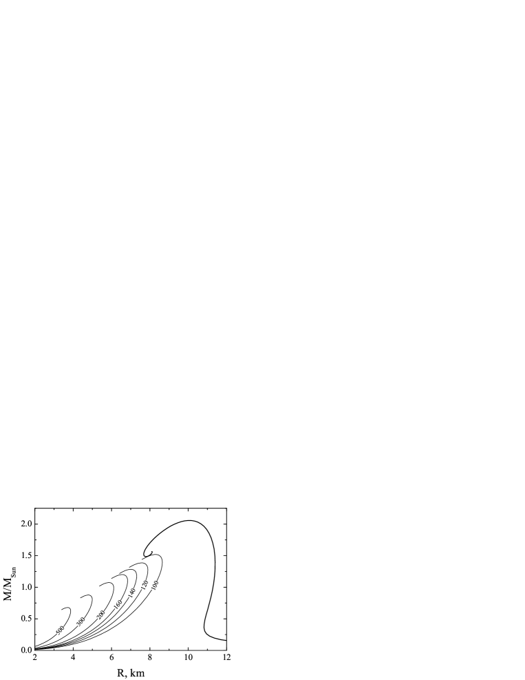
The diagrams relating the stellar mass and radius are applied to study the parameters of stellar models, in particular, their stability. An example of such a diagram is shown in Fig. 1. The thick line indicates the mass–radius relation for stars made of ordinary matter, without any phase transition. The thin lines correspond to purely quark stars containing no ordinary matter with their surface pressure and density . The numbers at the lines indicate the parameter in units of . A characteristic feature of the diagrams for quark stars is their passage through the coordinate origin . It should also be noted that all these mass–radius curves for quark stars are similar to one another (see the Section “Dimensionless Form of the Equations” below).
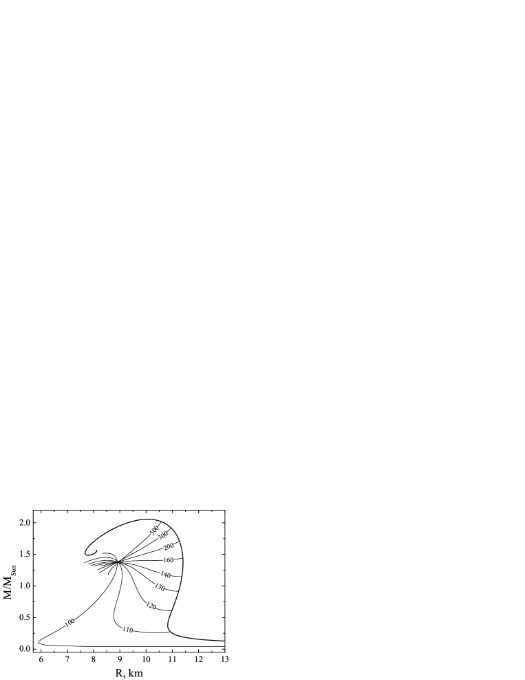
The mass–radius diagram for hybrid (i.e., containing both phases) stars calculated for our EOS is shown in Fig. 2. The thick line again indicates the dependence for the EOS without any phase transition to quark matter. The thin lines indicate these dependencies for various values of the parameter (the values of are indicated by the numbers in units of ). The density at which the phase transition begins is uniquely related to . This dependence is approximately described by the formula (see Yudin et al. 2013) , where — is the nuclear density and is measured in units of . For example, corresponds to , while for we have . The curve with at describes an almost pure quark star with a thin crust made of ordinary matter and, therefore, exhibits a dependence typical of such stars. On the other hand, as can be seen from the figure, all stars with quark cores at are unstable. Naturally, these specific values are unique to our model EOS.
Let us now turn to the formulation of the problem. As can be seen from Fig. 2, all curves with different B intersect in a very narrow region on the diagram (but not at a point!). This property, which is surprising per se, not only leads to some interesting consequences that we will discuss in conclusion but also undoubtedly requires an explanation. Actually, our paper is devoted to this explanation. Note also that such a behavior of the curves is not a unique property of precisely our EOS. the same effect can be seen, for example, in Fig. 15 from Schertler et al. (2000), in Fig. 4 from Fraga et al. (2002) and in Fig. 4 from Sagert et al. (2009).
Before turning to the main part of our work, we will emphasize once again the model status of our EOS. At present, the existence of neutron stars with a mass has been firmly established from observations (Demorest et al. 2010). As can be seen from Fig. 2, our EOS gives for the maximum mass of hybrid stars. Constructing the models of hybrid stars that satisfy observations is a separate, complex but accomplishable task (see, e.g., Weissenborn et al. 2011). For our purposes, it will suffice that the EOS used convey correctly the main characteristic properties of hybrid stars. In particular, we will show below that the linearity of the EOS for quark matter that is postulated in the bag model (Eq. (1)) but is also valid with a good accuracy in more sophisticated models (see, e.g., Zdunik and Haensel 2013; Bombaci and Logoteta 2013), which is needed for the existence of a “special point”, turns out to be a decisive property. In our view, the old result by Rhoades and Ruffini (1974), who found through variational calculations that precisely the linear EOS of the core maximizes the maximum neutron star mass for a known EOS of the crust, is remarkable in this context.
DERIVATION OF THE MAIN CONDITION
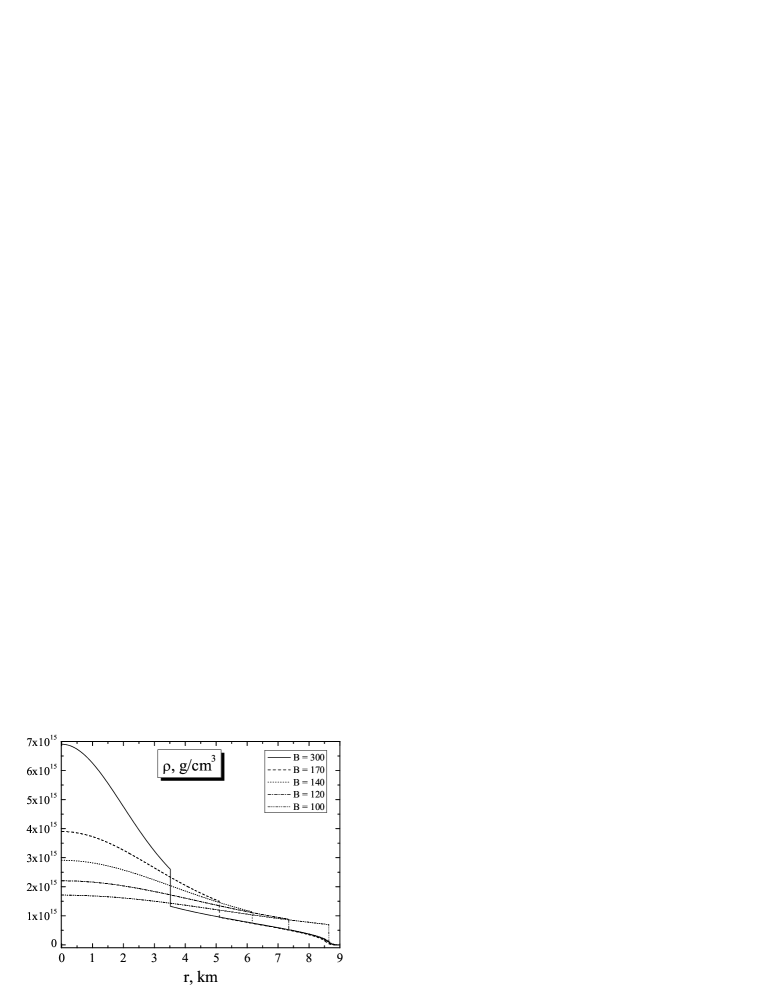
To come close to understanding the causes of the above effect, we need to compare the structures of stars near the point of intersection in Fig. 2. These stars corresponding to different values of the parameter B should have similar masses and radii. In Fig. 3 the baryon density of matter (, where is the baryonic charge density and is the atomic mass unit) is plotted against the radial coordinate . For each given value of , we chose a star near the point of intersection. As can be seen, these stars have a virtually identical crust made of ordinary matter to which a quark core is “stitched” at different depths, depending on the parameter . For example, the transition occurs at km for , at km for , etc. Thus, when changing the parameter , the quark matter–-ordinary matter boundary is shifted, leaving the crust virtually unchanged. Let us formalize this condition.
Let us first write the stellar equilibrium equations under general relativity conditions (the Tolman–Oppenheimer–Volkoff equations):
| (2) | ||||
| (3) |
where is the total (gravitating) mass within a sphere of radius . We will now denote the quantities referring to ordinary and quark matter by the subscripts 1 and 2, respectively. The phase equilibrium conditions at the boundary are reduced to the equality of the matter pressures and chemical potentials (everywhere below, we set the temperature equal to zero):
| (4) | |||
| (5) |
Recall that is the baryonic charge density. The EOS in the second phase can be written as
| (6) | |||
| (7) |
where is some parameter (in the case of quark matter, it is uniquely related to ). A change in leads to a change in the phase equilibrium parameters and , which are determined by varying Eqs. (4) and (5):
| (8) | ||||
| (9) |
Eliminating and from Eqs. (8) and (9) , we will find the relation between the change in pressure at the phase equilibrium point and the change in :
| (10) |
where we denote .
Let us now return to our star and suppose that it lies in the region where the curves in Fig. 2 intersect. A change in in phase 2 causes the phase boundary at to be shifted by ; in this case, according to the condition , only the central region with phase 2 changes, while the crust at remains unchanged. The change in pressure at the phase boundary can then be found as
| (11) |
where the pressure gradients are found from the Tolman–Oppenheimer–Volkoff equation (2). The last equality in (11) follows from (2) and the phase equilibrium condition (5). Similarly, the change in the mass coordinate of the phase boundary in the star is
| (12) |
where we again used Eqs. (4) and (5). The changes in the pressure and mass coordinate of the boundary of the core with phase 2 can also be found as
| (13) | |||
| (14) |
Here, the first term is attributable to the change in core radius, the second term is attributable to the change in central pressure and to the coordinated change in pressure at all points of the core caused by it, and the last term is attributable to the change in in the EOS of the central phase. We can now bring together the equations for (10), (11), (13) and (12), (14) and obtain a system of three equations for , and :
| (15) | ||||
| (16) | ||||
| (17) |
Since all of the quantities considered, except the parameter , refer to the second (central) phase, we omitted the subscript 2 here for brevity. For these equations to have a nonzero solution, the determinant of the system must become zero. This condition gives us the main equation
| (18) |
All of the quantities in this equation refer to the central phase (phase 2), because the parameter relating the phases dropped out of it. This remarkable fact implies that the property to conserve the total stellar mass and radius as the core size changes is determined only by the central phase and does not depend directly on the crust parameters! If condition (18) is met at some point of the star and if this point is the phase transition point (i.e., Eqs. (4) and (5) hold at it), then the total stellar mass and radius will not change at small variations in the parameter of the central phase.
DIMENSIONLESS FORM OF THE EQUATIONS
Let us now turn again to the case of stars with quark cores. As we have seen, the EOS for quark matter in the simplest case is a special case of the linear EOSs: with and . This fact allows the Tolman–Oppenheimer–Volkoff equilibrium equations (2) and (3) to be made dimensionless (for more details, see Haensel et al. 2007). More specifically, let us introduce dimensionless variables , and , with and ; in this case, . The equilibrium equations (2) and (3) will then be written as
| (19) | ||||
| (20) |
Having specified some central value of , , we can integrate these equations to the point , representing the surface of a quark star (). At fixed we obtain a family of solutions with the parameter .
Let us now rewrite the main equation (18) in dimensionless variables. Suppose that . Given that , we will then obtain
| (21) |
The derivatives with respect to the central pressure are
| (22) | ||||
| (23) |
Finally, the derivatives with respect to are expressed as
| (24) | ||||
| (25) |
Gathering all these expressions and replacing by its value from (20), we will obtain our main equation (18) in dimensionless form:
| (26) |
where can be determined from Eq. (19).
HOMOLOGOUS VARIABLES
To analyze Eq. (26) we will have to make a small digression. It is well known from the theory of polytropes that the system of stellar equilibrium equations (2) and (3) in the Newtonian limit with a polytropic EOS can be transformed to and by introducing the so-called homologous variables . These equations are reduced to one differential equation (see Chandrasekhar 1950). In this case, all solutions of the system with different central pressures (densities) fall on the same curve in the plane. It turns out that for an EOS of the form , the stellar equilibrium equations can also be similarly transformed within the framework of general relativity by introducing Milne’s homologous variables (see Chandrasekhar 1972; Chavanis 2002). However, the additional term in our expression violates homology. Nevertheless, we managed to find the variables in which the equilibrium equations (19) and (20) with the EOS are approximately homologous, i.e., their solutions fall virtually on the same curve in some domain of variables for moderately large (recall that in our case). Thus, let us introduce the variables and :
| (27) | ||||
| (28) |
The central point of the star corresponds to . The equations for and are:
| (29) | ||||
| (30) |
Naturally, only the second equation has the necessary homologous form. However, the first equation can also be brought to a homologous form in the limiting cases. First, let . This corresponds to , i.e. , the case where, according to what has been said above, a homologous solution definitely exists. To within terms instead of Eq. (29) we then have
| (31) |
where we expressed and in terms of , and using definitions (27) and (28). The third term in this expression containing the factor , is definitely small at the beginning of the homologous curve at and , where .
Consider the other limiting case of . To within , we then have
| (32) |
As we see, this expression coincides with the first two terms in (31). It is also interesting to note that the next expansion term, of order , is .

The thick solid spiral line in Fig. 4 indicates the result of our calculation according to Eqs. (30) and (31) (the limit ) and the dashed spiral (the limit ) corresponds to the solution according to (30) and (32). The structure of real quark stars (corresponding to the solution of Eqs. (19) and (20)) in homologous variables is indicated by the thin solid lines almost coincident with the spiral ones. The arrows indicate the points corresponding to the surface () of these stars; the number at the arrow indicates the corresponding dimensionless central density . As can be seen, all stars have a similar homologous structure in much of the plane; deviations are observed only in the region of the spiral turn. In this sense, our variables are actually “almost homologous”. The meaning of the thin dotted lines will be discussed below.
SOLUTION OF THE MAIN EQUATION
Let us now return to our main equation (26), which expresses the condition for the total stellar mass and radius being constant at small variations in the parameter of the central phase in dimensionless variables. The main problem is to find the derivatives and . Let us relate the quantities and to the homologous variables and :
| (33) | ||||
| (34) |
A change in the central density at leads to a change in the parameters and . However, no matter what this change is, it is just reduced to some shift along the homologous curve defined by the solution of the equation . Thus, we can write and , where the functions and are determined from Eqs. (29) and (30). Substituting this into the main equation (26), we obtain a cumbersome expression that, however, is simplified after some transformations to
| (35) |
Here and below, the asterisk marks the values of the quantities at the “special point”. This relation specifies the sought-for condition that the homologous variables and as well as the parameter should satisfy to serve as the solution of (26) (here, we expressed in the formulas in terms of , , and using (34)). In this case, and should lie on the homologous curve. The parameter on the diagram is a "hidden" variable, i.e., different values of correspond to the same values of and .
Consider the limiting cases of Eq. (35). First, let , i.e., the phase transition occurs in the crust, the star is virtually a purely quark one. The following condition should then be met:
| (36) |
which for leads to . This limit is indicated by the horizontal dotted line in Fig. 4. Its intersection with the homologous curve gives the corresponding . The other limiting case of gives an equation of the curve indicated by the oblique dotted line in Fig. 4:
| (37) |
Its intersection with the homologous curve occurs at and . Interestingly, these curves also pass through the limiting points of the corresponding homologous curves (the centers of the spirals corresponding to the solutions of the equations and (see (30), (32) and (31))). For example, the horizontal curve defined by Eq. (36) also passes through the limiting point of the homologous curve for with and , while the curve defined by Eq. (37) passes through the limiting point of the curve for with coordinates and (the numerical values are indicated for ).
Thus, all the states of interest to us lie in a small segment of the homologous curve: from to (see Fig. 4). Each point of this segment of the curve corresponds to some density ((according to Eq. (35)) between for the first above pair and for the second one. Accordingly, for each such point there exists such a unique value of that having begun the integration of the equilibrium equations (19) and (20) with this central density, we end up at the point with the required density . If the phase diagram of matter is structured in such a way that the phase transition occurs at this point, then such a star will have the sought-for property: its total mass and radius will not depend on small variations in the parameter (or ) of the central phase.
LARGE SCALE
The condition for the total stellar mass and radius being constant (18), its dimensionless form (26) and corollary (35) are local, i.e., they are valid only at small variations in the parameter (or ) of the central phase. In this case, the curves corresponding to various, slightly differing values of , on the mass– radius diagram intersect at a single point that we will call a “stationary point”. Naturally, different coordinates of the stationary points generally correspond to different values of . The line of stationary points on the mass–radius diagram is shown in Fig. 5. The numbers denote the corresponding values of in units of MeV/fm3. As can be seen, this curve has a rather peculiar shape. Owing to the two kinks at and the bulk of it occupies a bounded region of the diagram. This is one of the reasons why the mass–radius curves corresponding to different, even greatly differing values of , intersect in a small region (see Fig. 2). The second reason is related to the topology of the diagram: for example, the curves corresponding to small , whose stationary points lie above and to the left of the central triangle of stationary points run from bottom to top (as it should be for almost purely quark stars). The curves for intermediate run from right to left, while those for large drop from top to bottom and, passing through their stationary points, nevertheless also pass through the central zone of the diagram. Let us try to understand the behavior of the line of stationary points.

Consider a star with the parameters of the boundary of its quark core satisfying condition (35). Let us denote this condition by the relation and call the parameters that satisfy it the parameters of the stationary point. At a small change in and a corresponding change in the central density the total stellar mass and radius will remain unchanged. The core boundary now corresponds to new values of the dimensionless parameters, , and . If these values also satisfy the condition , then we can further change , conserving the total stellar mass and radius, etc. However, it is obvious that this is generally not the case and the new parameters need not be the parameters of the stationary point. Let us derive the condition under which the new state is also a stationary point. We have two relations: and , whence
| (38) | |||
| (39) |
where, as has already been said, the function is determined from Eq. (35).
Consider now how the parameters actually change during a shift that leaves the total stellar mass and radius unchanged. For this purpose, let us again return to Eqs. (10), (11) and (12), which relate the changes in pressure , mass and radius to the variation in . Writing them in dimensionless form and eliminating , we will obtain the relation
| (40) | |||
| (41) |
where we introduced the factor
| (42) |
The quantities , and are expressed in terms of , and using Eqs. (27), (33) and (34). To write the result in a compact form, let us split the quantities and as and , where (see also Eqs. (29) and (30))
| (43) | ||||
| (44) | ||||
| (45) | ||||
| (46) |
Here, in Eq. (29) we expressed in terms of , and using (34). We can now ultimately write the resulting relations in a compact form:
| (47) | ||||
| (48) |
where we introduced the common factor . These equations define how the dimensionless variables , and change during a shift that leaves the total stellar mass and radius unchanged. They should be compared with Eqs. (38) and (39), which define the shift between two stationary points. The requirement immediately leads us to Eq. (35). This means that if we are at a stationary point, then the shift will always be along the homologous curve irrespective of . The second equation leads us to a condition for :
| (49) |
If the jump in density satisfies condition (49), then the stationary point also remains stationary after the shift, i.e., the condition for the total stellar mass and radius being constant becomes global. Otherwise, when passing from one stationary point to another, the total mass and radius will slightly change. For our case, , and the parameters and lie within a narrow range from to . and respectively, correspond to them.
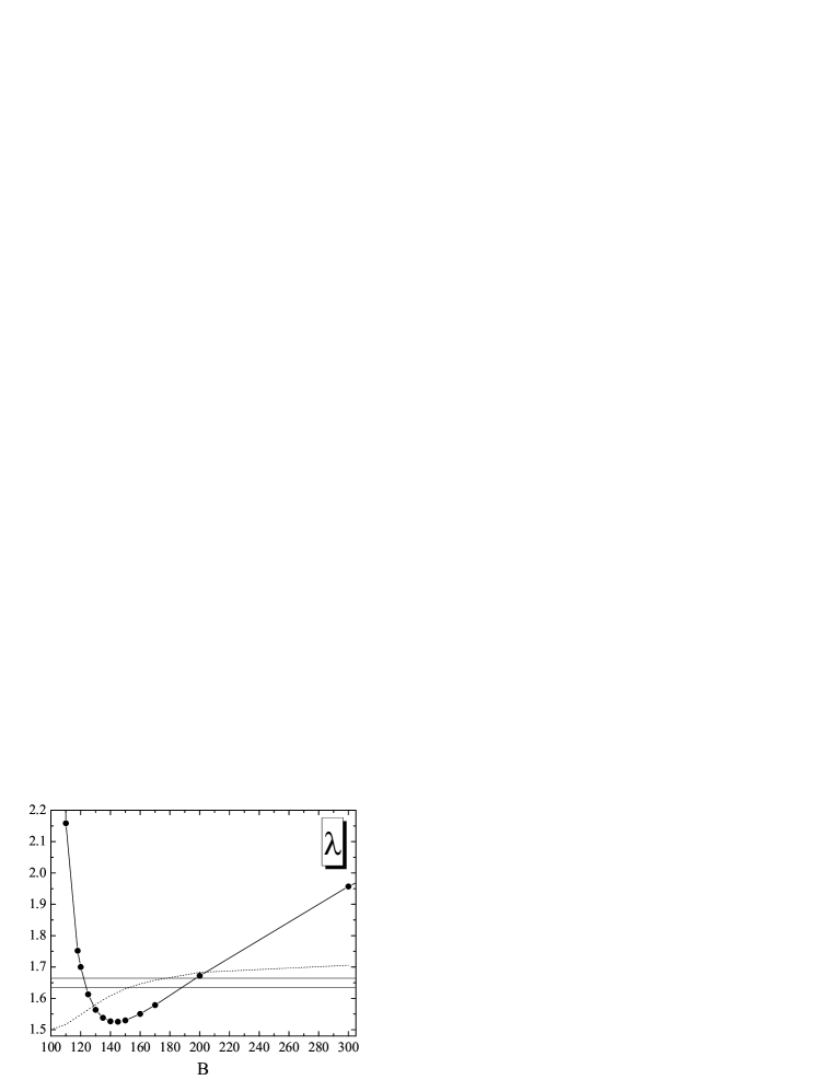
How does the dependence of on look in our case? Figure 6 gives the answer. It also shows the special values of listed above (solid horizontal lines) and the critical value of in the sense of the star’s stability (dotted line) that we will briefly discuss below. As can be seen, the narrow range of special values of breaks up the plot into several regions: in the zone , is larger than the special value and the line of stationary points runs downward on the mass– radius diagram (see Fig. 5). The region is special; here the property of stationarity is global, while the mass and radius are almost constant. This zone is the turning point in Fig. 6: further out, up to , is smaller than the special value and the line of stationary points in Fig. 5 changes its direction: now the radius drops, while the mass changes little with increasing . The region is again special and the turning one in Fig. 5. As increases further, increases and the line of stationary points runs monotonically to the upper right on the mass–radius diagram.
In conclusion, it remains for us to investigate two questions. First, what determines the coordinates of the “special point”, i.e., the characteristic mass and radius of the intersection region? As a reference point, we will take an almost purely quark star with (); the mass and thickness of the crust made of ordinary matter may be neglected (see Fig. (3)). Since , at its boundary, we can write Eqs. (27) and (28) in the following form by substituting the numerical values:
| (50) | ||||
| (51) |
Hence, passing to dimensional units, we will obtain the following characteristic values:
| (52) | ||||
| (53) |
The total stellar radius will be slightly larger, because there is also a tenuous “atmosphere” made of ordinary matter that makes virtually no contribution to the total mass (see Fig. 3). The plot of stationary points (Fig. 5) gives for the averaged coordinates of the point of intersection . It is interesting to compare this quantity with the results obtained in other works: for example, the point of intersection between themass–radius curves in Fig. 15 from Schertler et al. (2000) gives , Fig. 4 from Fraga et al. (2002) leads to , and Fig. 4 from Sagert et al. (2009) corresponds to . If, however, the approximation proposed in the book by Haensel et al. (2007) is used for the EOS of the crust within the framework of our approach, then we will obtain for the coordinates of the special point.
The second question concerns the phase transition parameter . This parameter defines the stability of a star when a new phase appears at its center: as Lighthill (1950) showed, its critical value in the Newtonian limit is ; at larger , stars with the phase transition at their centers are hydrodynamically unstable. This criterion was generalized to the case of general relativity by Seidov (1971) and took the form , where . It is easy to derive the relation
| (54) |
from Eqs. (4) and(5). Hence, for the critical value we have
| (55) |
where the last equality is valid, naturally, only for our linear EOS. It is this result that is indicated by the thin dotted line in Fig. 6. Remarkably, only the quantities referring to the central phase enter into the expression for . In addition, a condition for the parameters of interest to us can be derived from the equilibrium equations (4) and (5) and the requirement :
| (56) |
It bounds the range of at .
DISCUSSION AND CONCLUSIONS
Let us briefly summarize our main results: the existence of a special point on the mass–radius diagram of hybrid stars is a consequence of the combined action of several factors. First, the quark EOS for which the main local condition (18) was shown to be met because the equilibrium equations are homologous is linear. Second, the “phase diagram” of quark matter has peculiarities (see Fig. 6); as a consequence, much of the curve of stationary points lies in a small region of the mass–radius diagram (Fig. 5). Finally, the topology of the curves itself favors their intersection in a narrow region. Interesting questions arise here: First, will the property of intersection be retained on a global scale for a distinctly different phase diagram, i.e., at properties of the crust differing significantly from those considered? Second, are there solutions with other, nonlinear EOSs for our main (local) stationarity condition (18)? And, finally, the question touched on at the very beginning: how will our results change for the Gibbs description of the phase transition, where a region of mixed states appears instead of the sharp boundary between the phases in a star? These questions need to be investigated further.
Next, we established that the stars at the special point are “masked”, hiding their true structure under the veil of observable quantities ( и ). Consider this aspect of the problem. Let us adopt the linearity of the quark EOS and assume that we know the true EOS of nuclear matter without any phase transitions that gives a thick enveloping curve on the (see Figs. 1 and 2). Then, were it not the special point, only one measurement of the stellar mass and radius not only could say us whether such a star is a purely neutron or hybrid one (or, as a limiting case, a purely quark one) but could also point to the parameters of quark matter. However, the existence of a special point changes the situation: measuring the mass and radius of a star in its vicinity will only say us that this star contains a quark core, but neither its structure nor the parameters of quark matter will be determined. Either invoking additional information (for example, the cooling rate if the star was hot) or measuring the parameters of other hybrid stars to gain statistics and reconstruct the true curve will be required.
ACKNOWLEDGMENTS
This work was supported by grant no. 11.G34.31.0047 from the Government of the Russian Federation and SNSF SCOPES project no. IZ73Z0-128180/1. This work was also supported in part by the Russian Foundation for Basic Research (project nos. 11-02-00882-a, 12-02-00955-a, and 13-02-12106). We are grateful to the anonymous referees for their helpful critical remarks.
APPENDIX
Let us briefly describe the numerical method that we used to find the stationary points on the mass–radius diagram. Let we have a procedure that, starting from some central pressure (or, alternatively ), integrates the equilibrium equations (2) and (3) up to the surface defined by the condition . The stellar mass and radius being obtained in this case can be written as and , where the dependence on parameter is shown explicitly. For a small change in input parameters, we can, naturally, write
| (57) | ||||
| (58) |
At a stationary point, the equations and have nontrivial solutions and, hence, the determinant of the system
| (59) |
becomes zero. The derivatives in the determinant are easy to calculate numerically using several calls of the corresponding procedure and finite–difference equations. Thus, we obtain the function whose zeros specify the sought-for stationary points.
REFERENCES
1. I. Bombaci, D. Logoteta, Mon. Not. Roy. Astron. Soc. 433, L79–L83, (2013).
2. S. Chandrasekhar, An Introduction to the Study of Stellar Structure (Univ. of Chicago, Chicago, 1939; Inostr. Liter., Moscow, 1950).
3. S. Chandrasekhar, A limiting case of relativistic equilibrium, (Pergamon, Oxford, 1972)
4. P.-H. Chavanis, Astron. Astrophys. 381, p.709-730 (2002).
5. P.B. Demorest, T. Pennucci, S.M. Ransom, M.S.E. Roberts, J.W.T. Hessels, Nature 467, 1719, pp. 1081–1083, (2010).
6. F. Douchin, P. Haensel, Astron. Astrophys. 380, 151–167 (2001).
7. E.S. Fraga, R.D. Pisarsi, J. Schaffner-Bielich, Nucl. Phys. A, 702, 217-223 (2002).
8. P. Haensel, A.Y. Potekhin, D.G. Yakovlev, Neutron Stars 1. Equation of State and Structure, Springer, 619pp (2007).
9. M.J. Lighthill, Mon. Not. Roy. Astron. Soc. 110, 339–342, (1950).
10. T. Maruyama, S. Chiba, H-J. Schulze, and T. Tatsumi, Phys. Rev. D 76, 12, (2007).
11. C.E. Rhoades, R. Ruffini, Phys. Rev. Lett. 32, 324, (1974).
12. I. Sagert, M. Hempel, G. Pagliara, J. Schaffner-Bielich, T. Fischer, A. Mezzacappa, F-K. Thielemann and M. Liebendoerfer, J. Phys. G, 36, 6, (2009).
13. K. Schertler, C. Greiner, J. Schaffner-Bielich, M.H. Thoma, Nucl. Phys. A, 677, 1-4, 463-490 (2000).
14. Z.F. Seidov, Sov. Astron. 15, 347–348, (1971).
15. S. Weissenborn, I. Sagert, G. Pagliara, M. Hempel, J. Schaffner-Bielich, Astrophys. J. 740, 1, 5 pp, (2011).
16. A.V. Yudin, T.L. Razinkova, and D.K. Nadyozhin, Astron. Lett. 39, 161 (2013).
17. J.L. Zdunik, P. Haensel, Astron. Astrophys. 551, 8 pp, (2013).