A model-driven approach to broaden the detection of software performance antipatterns at runtime

Abstract

Performance antipatterns document bad design patterns that have negative influence on system performance. In our previous work we formalized such antipatterns as logical predicates that build on four different views: (i) the static view that captures the software elements (e.g. classes, components) and the static relationships among them; (ii) the dynamic view that represents the interaction (e.g. messages) that occurs between the software elements to provide system functionalities; (iii) the deployment view that describes the hardware elements (e.g. processing nodes) and the mapping of software resources onto hardware platforms; (iv) the performance view that collects a set of specific performance indices. In this paper we present a lightweight infrastructure that enables the detection of software performance antipatterns at runtime through the monitoring of specific performance indices. The proposed approach precalculates the logical predicates of antipatterns and identifies the ones whose static, dynamic and deployment sub-predicates occur in the current system configuration and brings at runtime the verification of performance sub-predicates. The proposed infrastructure leverages model-driven techniques to generate probes for monitoring the performance sub-predicates thus to support the detection of antipatterns at runtime.

1 Introduction

The model-based approaches, pioneered under the name of Software Performance Engineering (SPE) by Smith [28], create performance models and use quantitative results from these models to adjust the architecture and design [8] with the purpose of meeting performance requirements [31].

Several approaches have been successfully applied by modeling and analyzing the performance of software systems on the basis of predictive quantitative results [9]. However, the problem of interpreting the performance analysis results (such as mean response time, throughput variance) is still quite critical, since it is difficult to translate mean values, variances, and probability distributions into architectural feedbacks useful to overcome performance problems (such as split a software component in two components and re-deploy one of them). Such activities are still exclusively based on the analysts’ experience, and therefore they suffer lack of automation.

Software performance antipatterns [29] have been used to automate the interpretation of performance analysis results and the generation of architectural feedback [27, 32]. The rationale of using the performance antipatterns knowledge is two-fold: on one hand, an antipattern identifies a bad practice in the software architectural model that negatively affects the performance indices, and on the other hand, its definition also includes a solution description that lets the software architect devise refactoring actions. Hence, it is possible to identify from a bad throughput and/or utilization value the software components and/or interactions responsible for that bad value.

Since the software performance antipatterns had been originally defined in natural language, in [11] we have tackled the problem of providing a less ambiguous representation. Performance antipatterns are very complex (as compared to other software patterns) because they are founded on different characteristics of a software system, spanning from static to behavioral to deployment, and they additionally include values of performance indices. This high complexity requires multi-view representations, as demonstrated in [11].

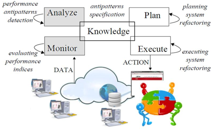
Figure 1: Antipattern-based MAPE process.

In this paper we move a further step ahead, in that we undertake the problem of detecting performance antipatterns at runtime. Inspired by the IBM autonomic control loop [14], Figure 1 schematically represents the operational steps of the antipattern-based reconfiguration process we propose. The overall process of Monitoring, Analyzing, Planning, and Executing (MAPE) is executed to assess and, if needed, improve the performance properties of a software architecture under development. Software architectures are characterized by a huge amount of interactions among software elements; such interactions are input to the antipattern-based process whose goal is to provide and make use of knowledge. Shaded boxes of Figure 1 represent the focus of this paper. In particular, our approach supports two main activities: (i) Monitor, i.e. the monitoring of performance indices; (ii) Analyze, i.e. the detection of performance antipatterns. After detecting antipatterns, there are two activities that must be executed to complete the feedback process: (i) Plan, i.e. the antipattern-based reconfiguration actions are planned; (iv) Execute, i.e. the system is reconfigured by removing the detected antipatterns.

The goal of this paper is to broaden the detection of software performance antipatterns at runtime by introducing a model-driven monitoring infrastructure able to measure a specific set of performance indices. To this end, we introduce a model-based approach that allows to precalculate the logical predicates of performance antipatterns and identifies the ones whose static, dynamic and deployment sub-predicates occur in the system configuration under analysis. The proposed infrastructure leverages model-driven techniques to generate probes for the verification of performance sub-predicates by monitoring a sub-set of performance indices only.

The paper is organized as follows. Section 2 provides some background information on software performance antipatterns. The process for the detection of antipattern at runtime is described in Section 3. Section 4 presents the monitoring infrastructure we use to verify performance sub-predicates. Section 5 shows the approach at work on a case study. Section 6 discusses the related works, and finally in Section 7 conclusions and future research directions are sketched.

2 Performance Antipatterns

Figure 2 reports the formalization we provided in [11] for Blob, the Circuitous Treasure Hunt (CTH), and the Traffic Jam (TJ) antipatterns. As mentioned in Section 1, antipatterns are founded on different characteristics of a software system that we organized in four different views: (i) the static view S that captures the software elements (e.g. classes, components) and the static relationships among them; (ii) the dynamic view Dy that represents the interaction (e.g. messages) that occurs between the software elements to provide the system functionalities; (iii) the deployment view De that describes the hardware elements (e.g. processing nodes) and the mapping of software resources onto hardware platforms; (iv) the performance view P that collects a set of specific performance indices.

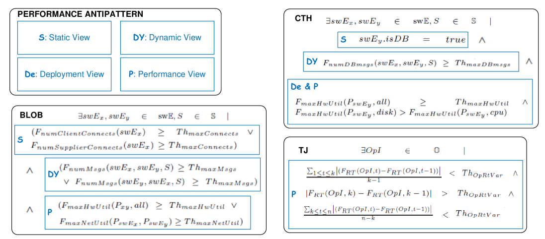
Figure 2: Performance antipatterns modeling.

To determine when performance antipatterns occur, our specification includes thresholds on design (i.e. static, dynamic and deployment) features (e.g. many usage dependencies, excessive message traffic) and performance indices (e.g. high, low utilization).

For example, a Blob occurs when a component requires a lot of information from other ones, it generates excessive message traffic that lead to over utilize the device on which it is deployed or the network involved in the communication. Its logic-based representation is reported in Figure 2 where four thresholds have been defined: (i) $Th_{maxConnects}$ indicates the maximum number of connections a component may be involved in; (ii) $Th_{maxMsgs}$ indicates the maximum number of messages a component may send in an interaction; (iii) $Th_{maxHwUtil}$ indicates the upper bound for processing device utilization; (iv) $Th_{maxNetUtil}$ indicates the upper bound for network device utilization. The first two thresholds refer to static and dynamic features, respectively, whereas the latter ones refer to performance indices. As another example, a TJ occurs when one problem causes a backlog of jobs that results in a wide variability in response time. Its logic-based representation is reported in Figure 2 where one thresholds has been defined: (i) $Th_{OpRtVar}$ indicates the maximum bound for the variability in response times of operations across time intervals, and it refers to a performance index.

Each antipattern is formalized by a set of sub-predicates referring to the defined four views, as depicted in Figure 2. Note that there are some antipatterns whose predicates span on all the four views (such as CTH), some others referring to a sub-set of views (such as Blob) and finally there are some antipatterns whose predicates refer to the performance view only (such as TJ). Besides the TJ, there are three other antipatterns (over a set of twelve antipatterns we formalized in [11]) that refer to the performance view only in their modeling, i.e. ’Concurrent Processing System’ (CPS), ’The Ramp’, and ’More is Less’. For more details on these antipatterns please refer to [11].

3 Performance Antipattern Detection: Process at Runtime

In this section we describe the process we envisage for the detection of performance antipatterns at runtime. To speed up the detection activity, our process is constituted by two main operational steps: (1) a full automatic pre-calculus of antipatterns that off-line determines the set of antipatterns instances for which the current running configuration satisfies the static, dynamic, and deployment views; (2) monitoring of performance indices for the set of antipatterns instances identified during the pre-calculus step. In this way the effort spent by the monitoring is reduced since we perform at runtime the verification of a, possibly limited, sub-set of antipattern instances only.

We recall that there are four antipatterns whose logical formula includes the performance view predicates only (see Section 2), hence the pre-calculus step is not executed for them. The detection of these antipatterns is due to a set of performance indices that must be always monitored at runtime.

Figure 3 illustrates how the system configuration ($SC$) is modified over time while detecting and solving performance antipatterns. In a generic instant of time $t_{i}$ a system configuration $SC_{i}$ is constituted by three elements: {$S_{i}$, $PA_{i}$, $M_{i}$[$PA_{i}$]}, where $S_{i}$ represents the running system, $PA_{i}$ is the set of antipattern instances whose (static, dynamic, deployment) views have been already verified in $S_{i}$, and $M_{i}$ represents the active monitors generated on the basis of $PA_{i}$ that must check the verification of their performance view predicates.

Figure 3: System Configuration, Antipatterns Instances and Active Monitors over time.

The detected antipatterns constitute the knowledge on which refactoring actions are devised. In particular, two different types of refactorings can be considered at a generic instant of time $t_{i}$: software and hardware refactorings. Software refactoring generates a new system configuration ($SC^{\prime}_{i+1}$) where the running configuration is modified ($S^{\prime}_{i+1}$) and the pre-calculus step returns a new set of instances ($PA_{i+1}$) together with a new set of active monitors $M_{i+1}$[$PA_{i+1}$]. Some examples of software refactoring are: (i) the splitting of software components, (ii) the redeployment of software components into different hardware platforms, (iii) the replacement of software components with ones that require lower amounts of resource demands, etc. By hardware refactoring we consider all the refactoring actions that do not modify the (static, dynamic, deployment) characteristics of software systems thus to skip the pre-calculus step since the set of antipatterns and active monitors do not change. Some examples of hardware refactoring are: (i) the increasing of the processing power of processors, disks, and/or network resources, (ii) the increasing of the multiplicity of processors, disks, and/or network resources, etc. Note that software/hardware refactorings may incur different costs thus inducing a quality trade-off issue. For the sake of simplicity, we do not consider this issue here.

4 Property-Driven Monitoring Infrastructure

In this section we describe the monitoring infrastructure that evaluates the antipatterns performance view. We recall that this latter view is represented by a set of performance properties the running system must manifest during its execution to detect the corresponding antipattern. Such predicates are generally defined for each antipattern (see Section 2) but must be actualized for the specific system under analysis. For example, the TJ antipattern occurs under specific conditions related to the response time ($F_{RT}$) of one operation instance ($OpI$) at a given time $t$. The actual detection of the TJ antipattern at runtime includes the specification of the generic $OpI$ that, customized for a specific system, become the actual operation instance that needs to be monitored.

The monitoring infrastructure we propose takes advantage of model-driven techniques since the set of performance antipatterns to detect (and the corresponding properties to monitor) can change at runtime (see Section 3). In particular, the process must be iterated each time the properties to be monitored change, hence a substantial human effort and specialized expertise is required if the high level description of system properties must be translated into lower-level monitor directives. Our model-based infrastructure builds upon a property-driven monitoring framework we proposed in [4], and it automatically translates the predicates of antipatterns performance view into a concrete monitoring setup.

The sequel of the section discusses the performance view properties modeling approach in Section 4.1, and presents the configurable monitoring infrastructure we propose for the monitoring activity in Section 4.2.

4.1 Performance view properties modeling approach

Figure 4 illustrates our performance view properties modeling approach. Both Generic and Actual properties are modeled by using the Property Meta-Model (PMM) [19, 6], and the corresponding models are conform to it (C2 relation in Figure 4). Generic Property Models are defined once and are generic w.r.t. the events to observe, whereas Actual Property Models, being heavily-coupled with the specific system to monitor, are specified time by time when the thresholds and the events to be observed are determined and the running system configuration ($SC_{i}$) is known.

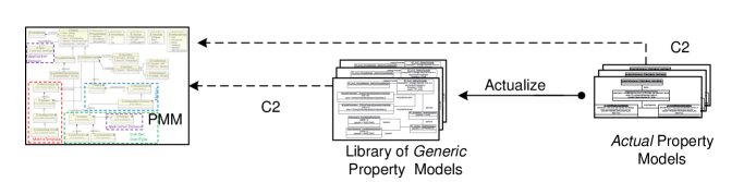
Figure 4: Performance View Properties Modeling Approach.

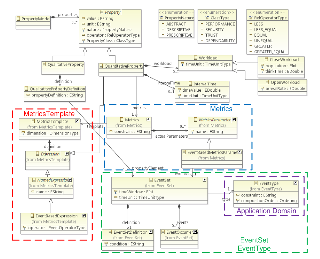
Figure 5: PMM structure.

Note that the Generic Property Models represent a pre-defined Library we built from the logic-based representation of antipatterns discussed in Section 2, and the Actual Properties Models are obtained by actualizing the Generic Property Models (Actualize relation in Figure 4) to the specific system.

The actualization step is not fully automatic: while the events to observe are provided by the pre-calculus, the thresholds on performance indices must be initially set by experts and, possibly, dynamically adapted by considering specific heuristics on observed performance values.

Property Meta-Model

Figure 5 reports the PMM key concepts and their relationship. PMM includes PRESCRIPTIVE and DESCRIPTIVE properties of systems. A property can be qualitative (QualitativeProperty) or quantitative (QuantitativeProperty). In general, quantitative properties are related to performance or dependability, whereas QualitativeProperty refers to properties about the event occurrences that are observed and cannot be measured. They in general refer to the behavioral description of the system (e.g. deadlock freeness or liveness). Quantitative properties are measurable and have associated Metrics. A QuantitativeProperty can be associated to a Workload and/or an IntervalTime.

MetricsTemplate models a generic metric (e.g. the response time as the duration of an event/operation), the concrete Metrics that refers to a MetricsTemplate and specifies the (actual) metricParameter for the (formal) templateParameter in the application domain the metric has been defined. The specification of the concrete event in the metric is done via the EventType the metric refers to. Such EventType refers to observable operations or events belonging to the Application Domain for which the Property needs to be verified/guaranteed. An EventSet represents a set of event instances the refer to the same EventType.

PMM is implemented as an eCore model using Eclipse Modeling Framework (EMF) [12] and it is provided with an associated editor realized as an Eclipse Plugin. This editor allows to create new model instances of the Property, Metrics, MetricsTemplate, EventType and EventSet meta-models.

Library of Generic Property Models

Figure  6 shows an example of a generic property model in the library, namely TJPropertyModel, modeling the TJ antipattern performance predicate (at the left-hand of the figure) and the average response time MetricsTemplate used in it (at the right-side of the figure).

The TJPropertyModel contains three QuantitativeProperty models, one for each term of the performance predicate. The three QuantitativeProperty models refer to the same property on different time slots, hence for the sake of space, we only describe the AVG-TR-1-k-Property. This is a PERFORMANCE PRESCRIPTIVE property with two parameters, $RT-AVG-OpI-1-k and $Th_OpRtVar. The former refers to the metrics to be used for the specific operation, whereas the latter parameter indicates the threshold for the average response time of the operation. Furthermore, AVG-TR-1-k-Property has a generic closedWorkload with two parameters to be actualized: $p representing the population of the closedWorkload and $Th the think time of each individual of the population. To obtain an Actual Property Model for the TJ antipattern, all the parameters of the TJPropertyModel need to be actualized to a concrete scenario.

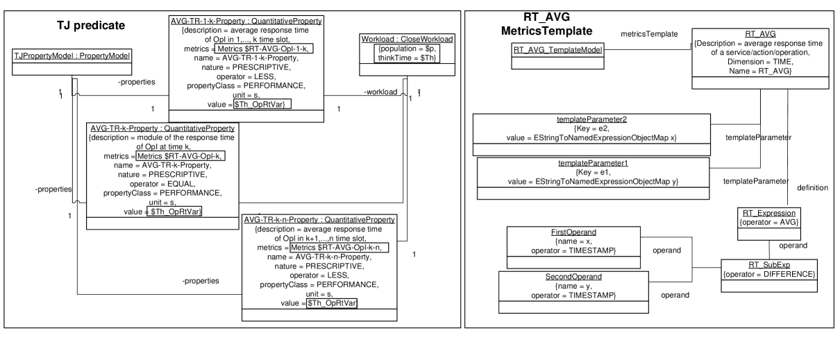
Figure 6: Traffic Jam Performance Predicate and Response Time Metrics Template.

$RT\_AVG$ MetricsTemplate represents a TIME measure defined as average of the differences for the timestamps of two generic event instances ($x$ and $y$ in the model). The template exposes two templateParameters: $e_{1}$ bound to $y$, and $e_{2}$ bound to $x$. A Metrics, whose definition is an instance of the MetricsTemplate, concretises the template for a specific scenario. This is reflected in the metrics’ actual parameters which substitute the template parameters by linking the general description to the specific application domain the metrics refers to. We will see in Section 5 the RT_updateVitalParameters_Metrics that actualizes the corresponding $RT\_AVG$ MetricsTemplate by linking to the templateParameters $e_{1}$ and $e_{2}$, two EventSets ($startUpVitalPar\_Set$ and $fwAckVitalParameters\_Set$ respectively), and specifying that the two event sets must satisfy a metrics constraint (i.e. the two event sets must be related to each other).

4.2 Configurable Monitoring Infrastructure for Antipattern Detection

Figure 7 depicts our configurable monitoring infrastructure. It is composed by: i) a generic monitoring framework (i.e. GLIMPSE [5]), and ii) a PMM-2-Drools Translator that generates DROOLS rules from PMM Actual Property Models, and such rules are used to configure GLIMPSE to the actual properties to monitor at run time.

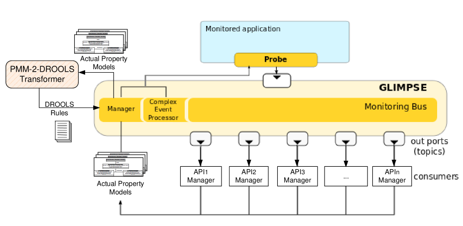
Figure 7: Property-Driven Monitoring Infrastructure for Antipattern Detection.

As shown Figure 7, the GLIMPSE manager component takes as input the property model and activates an external component that performs the code generation according to Drools Fusion complex event processor [2]. The output of this transformation is represented by a specific rule that is processed by the complex event processor component of GLIMPSE. In this way, we configure the generic framework GLIMPSE to a concrete monitoring infrastructure.

Generic fLexIble Monitoring based on a Publish-Subscribe infrastructurE (GLIMPSE)

As shown in Figure 7 GLIMPSE, developed with the goal of decoupling the event specification from the analysis mechanism, is composed of five main components:

Probes that intercept primitive events when they occur in the software and send them to the GLIMPSE Monitoring Bus. Probes are usually realized by injecting code into an existing software or by using proxies. The generated Drools rules are used from the Manager to instruct the probes for monitoring the system characteristics of predicates belonging to the antipatterns performance view. Note that the probes instrumentation strictly depends on the Actual Property ($AP_{i}$) precalculated for the system configuration $SC_{i}$ (see Section 3).

Monitoring Bus that is the communication backbone that all information (events, questions, answers) is sent on: Probes, Consumers, Complex Event Processor and by all the services querying information to GLIMPSE. A publish-subscribe paradigm devoting the communication handling to the Manager component is here adopted.

Complex Event Processor (CEP) is the rule engine which analyzes the primitive events, generated from the probes, to infer complex events matching the consumer requests. There are several rule engines that can be used for this task. The current GLIMPSE implementation adopts the Drools Fusion rule language [2].

Consumer that is a simple customer requiring some information to be monitored. It sends a request (Actual Property Model) to the Manager using the Monitoring Bus and waits for the evaluation results on a dedicated channel provided by the Manager. Consumers are software components that manage the antipattern instances to detect and solve. In particular, we have one AP Manager for each antipattern instance in $PA_{i}$ of the system configuration $SC_{i}$ (as defined in Section 3).

Manager that is the orchestrator of the GLIMPSE architecture. It manages the communications among the GLIMPSE components. Specifically, the Manager fetches requests coming from Consumers, analyzes them and instructs the Probes. Then, it instructs the CEP Evaluator, creates and notifies to the Consumer a dedicated channel on which it will provide results produced by the CEP Evaluator.

PMM Model to DROOLS Rules Translator

The translation of the PMM model into Drools rules automatizes the GLIMPSE configuration transforming the PMM models into a concrete monitoring setup. The Model2Code Transformer component has been implemented using the Acceleo code generator IDE [3] that supports the automated code generation from UML and EMF and uses the templates to generate code (or text) from a model.

The implemented Model2Code Transformer has a .mtl extension, it takes as inputs the PMM ecore models (specifically Core.ecore, EventSet.ecore, EventType.ecore, Metrics.ecore, MetricsTemplate.ecore, Property.ecore) and the model (compliant to PMM) of the property, metrics or event to be monitored, and produces as output one or more Drools rules, that are provided in input to the GLIMPSE complex event processor.

The Transformer consists of a main generation rule or template that calls a certain number of other templates, each one is applied on a PMM model element (or object) to produce some text. In each template there are static areas, and they will be included in the generated file as they are defined, whereas dynamic areas correspond to the expression evaluation on the current object.

Listing 1: Main Template of Model2Code Transformer

⬇

[comment encoding = UTF-8 /]

[module generate(’cpmm/model/Core.ecore’,’cpmm/model/EventType.ecore’,’cpmm/model/EventSet.ecore’,’cpmm/model/Metrics.ecore’,’cpmm/model/MetricsTemplate.ecore’,’cpmm/model/Property.ecore’)]

[import cpmm::acceleo::utilities::utility]

[template public generateElement(p : Property)]

[comment @main/]

[file (p.name, false, ’Cp1252’)]

[if p.oclIsTypeOf(QuantitativeProperty)]

[processMainQuantitativeProperty(p)/]

[elseif (p.oclIsTypeOf(QualitativeProperty))]

[processQualitativeProperty(p)/]

[/if]

[/file]

[/template]

As showed in Listing 1, the heading section defines which meta-model the template will apply for and the generated file, and a main template (called generateElement) is defined to represent the main generation rule. It takes as input the property model and if this model is about a quantitative property then a specific template named processMainQuantitativeProperty is called, otherwise the processQualitativeProperty is called. The processMainQuantitativeProperty calls a specific template processing the associated metrics. In this template the Metrics model is navigated for identifying the associated MetricsTemplate model, then the MetricsTemplate parameters, the associated EventBasedExpressions and their operators. These EventBasedExpressions represent expressions based on events and their name represents the observable, simple or complex, event/behavior the operator applies to.

5 Case Study: E-Health System

The E-Health System (EHS) supports the doctors’ everyday activities, such as the retrieval of information of their patients. On the basis of such data they may send an alarm in case of warning conditions. The patients are allowed to retrieve information about the doctor expertise and they update some vital parameters (e.g. heart rate) thus to provide the knowledge aimed at monitoring their health. The service we analyze in the following is the UpdateVitalParameters, since it is required by a large number of users that originate a huge number of processes at approximately the same time.

To conduct this proof of concept, we adopt a model-based performance analysis. However, the presented approach remains feasible for any running system. We model EHS with UML [24] profiled with MARTE [25]. Figure 8 reports an excerpt of the EHS component and deployment diagrams illustrating the software components and their interconnections, and the deployment of the software components on the hardware platforms. The client application has been deployed on a Personal Digital Assistant (PDA), i.e. a mobile device in the hands of patients.

Figure 9 reports the sequence diagram for the UpdateVitalParameters service. It describes the communication between software components for the UpdateVitalParameters service: a opt fragment indicates that at 6 p.m. patients need to update their vital parameters hence their client application sends a request to the application server that is meant to manage the communication towards the database. Vital parameters of patients are sent to the database, stored on it and, afterwards such update is notified to the client and visualized to the patient.

Figure 8: EHS- UML Component and Deployment Diagram.

The sequence diagram of Figure 9 contains annotations that will be used in the model-based performance analysis. For example, the setVitalParameters is annotated with the MARTE stereotype GaScenario through which it is possible to specify the usage of hardware resources: in particular it requires: (i) 20 instructions from a cpu device, and (ii) 10 accesses from a disk device. The workload addressed to hardware resources is calculated as the sum of demands, hence in this case the patient’s device executes $25$ cpu instructions (20 for setVitalParameters plus $5$ for fwdAckVitalParameters) and $10$ disk accessed (10 for setVitalParameters plus 0 for fwdAckVitalParameters). Consider as another example of annotations that the communication between the patient’s device and the AppHost requires to exchange over the network a message of size equal to $6$ Mbit.

A performance requirement has been defined on the RT(UpdateVitalParameters) service, i.e. such service has to be offered in less than 0.5 seconds, while considering a workload of ten thousands patients with a thinking time equal to 86400 seconds, i.e. patients update their vital parameters each day.

The model-based performance analysis phase has been conducted as follows. We used the Prima-UML methodology [10] to automatically derive a Queueing Network (QN) [18] starting from the UML models related to the UpdateVitalParameters service. The QN has been analyzed with JMT [7].

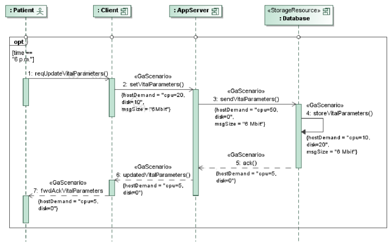
Figure 9: EHS- UML Sequence Diagram for the UpdateVitalParameters service.

The obtained QN model has a set of queueing centers (e.g. cpu-PDA) representing the hardware resources of the system, and a set of delay centers (e.g. WAN) representing the network delays. The input parameters adopted for this experiment are reported in Table 2: the first column lists the QN service centers; the second column shows the average service demands for the class of job under analysis.

We have referred to [13] for typical performance parameters, like processors, disks and networks latencies. For example, in Table 2 we can see that the cpu-PDA queueing service center requires 0.00375 ms and it is obtained from $0.000015*25$ in which 0.000015 ms represents the service time of a microprocessor multiplied for the number of cpu instructions (25, as stated in the sequence diagram of Figure 9). Network communication links are subjected to the message size, in fact in Table 2 we can see that the WAN delay center requires 500 ms and it is obtained from $6/0.012$ in which 6 Mbit represents the size of the message exchanged over the network (see Figure 9) and it is divided for the service time of a wired area network (12 Mbit/sec).

Service Center	Input parameters
cpu-PDA	0.00375 ms
disk-PDA	57 ms
WAN	500 ms
cpu-AppHost	0.00825 ms
LAN	60 ms
cpu-DbHost	0.00225 ms
disk-DbHost	114 ms

Table 1: EHS- QN model input parameters.

antipattern	parameter	value
	$Th_maxConnects	4
Blob	$Th_maxMsgs	5
	$Th_maxHwUtil	0.8
	$Th_maxNetUtil	0.7
	$Th_initSlot	0
TJ	$Th_sizeSlot	50
	$Th_endSlot	1500
	$Th_OpRtVar	0.3

Table 2: EHS- parameters binding.

Our model-based performance analysis predicts that the system offers the UpdateVitalParameters service with an average time of 0.61 seconds that is greater than the required 0.5 seconds. Hence, the unfulfillment of the requirement triggers the detection of performance antipatterns.

Antipattern-based detection rules contain parameters that need to be actualized on the analyzed model and basically represent thresholds that formalize system features. We provide heuristics to estimate their numerical values. For example, Table 2 report the thresholds we consider for Blob and TJ antipatterns. Such values allow to actualize the parameterized detection rules into instantiated ones, thus proceeding with the actual detection. The TJ antipattern requires four thresholds: $Th_initSlot and $Th_endSlot define the initial and the final instant of the observation time slot, whereas $Th_sizeSlot represents the width of the sub-intervals considered in the evaluation of performance indices; $Th_OpRtVar is used to specify the upper bound for the service response time slope between two sub-intervals. The binding of these thresholds is intrinsically more difficult than others, and the numerical values are set by exploiting historical data (obtained by previous performance analysis) to accurately tune the slope used as boundary for the increase of the response time.

Then, we apply our process to detect performance antipatterns. The pre-calculus verifies the static, dynamic, and deployment characteristics of performance antipatterns, and pointed out that: (i) the AppServer component may originate an instance of the Blob antipattern in the EHS model since it (see Table 2 and Figure 8) has more than 4 connections towards other components, sends more than 5 messages in the PatientInfo service, and is deployed on a different node with respect to the Database component, hence the LAN utilization need to be monitored. In this way for the Blob antipattern the monitoring of performance indices is limited to the LAN utilization. In our case study, $SC_{0}$ = {$EHS$, {Blob, TJ, CPS, The Ramp, More is Less}, {Utilization(LAN), RT(UpdateVitalParameters), …}}.

Our property-driven monitoring infrastructure transforms the generic property models corresponding to the pre-calculated antipatterns into the EHS actual property models. Figure 10 shows the actual property model for TJ performance view obtained by actualizing the generic property model used in TJ performance sub-view (see Figure  6). In particular, the actual TJ property sets the workload parameters (population to 10000 and thinking time to 86400), the threshold value to 0.3 and the average response time metrics related to the EHS UpdateVitalParameters operation instance that is reported in the model of the right-side of the figure. The derived actual property model is sent to GLIMPSE that, invoking the translator, obtains the Drools rules, thus to instruct the probes. Then, the monitoring infrastructure starts to monitor the occurrences of the pre-calculated antipatterns.

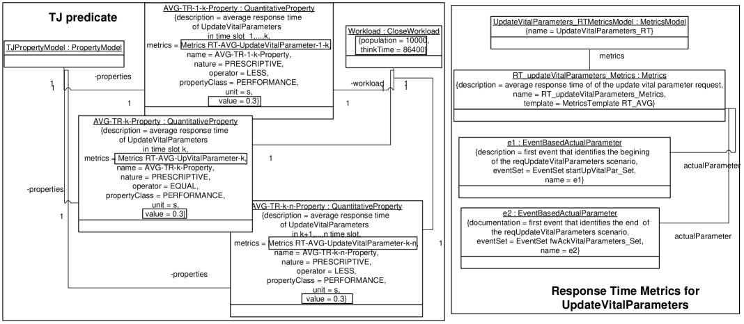
Figure 10: EHS- actual property model for the TJ antipattern.

In the following we report the data of RT(UpdateVitalParameters) that provided the evidence for the TJ antipattern occurrence. Figure 11 illustrates the trend of the average response time for the UpdateVitalParameters service (y-axis) over time (x-axis) while fixing the workload to ten thousand patients. We obtained this trend by following the antipattern thresholds (see Table 2): (i) the time starts at the interval $0$; (ii) the size of the intervals is fixed to $50$ seconds; (iii) the time ends after $1500$ seconds; (iv) for each interval we calculated the average response time of the observed completions and we verify if the slope among two intervals is larger than 0.3 seconds. For example, in Figure 11 there are several subsequent intervals that violate the threshold, e.g. in the interval from 300 to 350 seconds the average response time is 0.81 whereas the interval from 350 to 400 seconds the average response time is 1.27 hence the slope is 1.27 - 0.81 = 0.46 (larger than 0.3). Hence, we can assert that the TJ antipattern occurs in the UpdateVitalParameters service since several subsequent intervals differ with values larger than the antipattern threshold.

The TJ antipattern is solved by substituting the hardware platform (DbHost) hosting the database component with a new one whose processing power is increased by a factor of 1/100. Such refactoring action, i.e., the replacement of the DbHost hardware platform with a faster one, is a hardware refactoring (see Section 3) and leads to a system configuration $SC_{1500}$ = {$EHS$, {Blob, TJ, CPS, The Ramp, More is Less}, {Utilization(LAN), RT(UpdateVitalParameters), …} }. where no changes have been performed to the set of antipatterns and active monitors. The software model, refactored with the TJ antipattern, has been newly analyzed and we found that such refactoring action was beneficial in fact the response time of UpdateVitalParameters service significantly improves. The requirement has been fulfilled, in fact even while considering a workload of ten thousands patients the system offers the service in an average time of 0.5 seconds, as stated in the requirement.

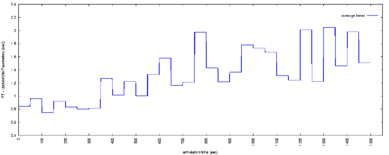
Figure 11: EHS- the TJ antipattern occurrence.

6 Related Work

Several approaches have been recently introduced to specify and detect code smells and antipatterns [23, 16]. They range from manual approaches, based on inspection techniques [30], to metric-based heuristics [26], using rules and thresholds on various metrics [22] or Bayesian Belief Networks [17].

Parsons et al. [27] present a framework for detecting performance antipatterns, where a rule-based performance diagnosis tool, named Performance Antipattern Detection (PAD), is presented. The approach deals with Component-Based Enterprise Systems, targeting Enterprise Java Bean (EJB) applications only. It is based on monitoring data from running systems, it extracts the runtime system design and detects EJB antipatterns by applying rules to it. However, the scope of [27] is restricted to such domain (i.e. EJB running applications), and the detection of the performance problems is not allowed earlier in the development process. In complement, our approach intends to work at the design level and it can be applied early in the software life-cycle.

In our previous work we first tackled the problem of providing a more formal representation for performance antipatterns [29] by introducing first-order logic rules that express a set of system properties under which an antipattern occurs [11]. We also started to investigate the problem of providing QoS-based feedback by means of design and runtime knowledge in [21]. On the contrary, in this paper we focus on how the runtime knowledge can be used for the detection of software performance antipatterns.

Besides antipatterns-based approaches, there is some literature that deals with the automated generation of architectural feedback, in particular: (i) rule-based approaches (e.g. [15]) encapsulate general knowledge on how to improve system performance into executable rules; (ii) design space exploration approaches (e.g. [33]) explore the design space by examining alternatives that can cope with performance flaws; (iii) metaheuristic approaches (e.g. [20]) make use of evolutionary algorithms looking for design alternatives aimed at improving the system performance.

7 Conclusions

In this paper we presented a model-driven approach that allows the detection of software performance antipatterns at runtime. In particular, the process we proposed for the detection of performance antipattern at runtime is composed by two steps: pre-calculus and monitoring. For the second step, we proposed an adaptation of a monitoring infrastructure, built on top of a property meta-model (PMM), that has been presented in [4]. From models conform to PMM it is possible to generate Drools Rules that are interpreted by the generic monitoring framework GLIMPSE. In this way, it is possible to instruct the monitoring infrastructure to concrete set up. The benefit of our approach is the introduction of a pre-calculus step that partially evaluates the antipattern logic formulation, checks off-line the static, dynamic, and deployment characteristics of antipatterns, and only leaves the verification at run time of the performance view predicates to the monitoring infrastructure.

Our future work agenda is represented by the following tasks: (i) complete the library of the Generic Property Models; (ii) extensively validate the PMM2DROOLs transformation in order to test its correctness in several scenarios; (iii) evaluate the overhead of the GLIMPSE rule engine w.r.t. compiled probes; (iv) experiment the approach on case studies coming from industrial experiences.

References

- [1]
- [2] Drools Fusion: Complex Event Processor. http://www.jboss.org/drools/drools-fusion.html.
- [3] Acceleo: http://www.eclipse.org/acceleo/.
- [4] A. Bertolino, A. Calabrò, F. Lonetti, A. Di Marco & A. Sabetta (2011): Towards a Model-Driven Infrastructure for Runtime Monitoring. In: SERENE, LNCS 6968, Springer, pp. 130–144. Available at http://dx.doi.org/10.1007/978-3-642-24124-6_13.
- [5] A. Bertolino, A. Calabrò, F. Lonetti & A. Sabetta (2011): GLIMPSE: a generic and flexible monitoring infrastructure. In: Proceedings of EWDC, pp. 73–78. Available at http://doi.acm.org/10.1145/1978582.1978598.
- [6] A. Bertolino, A. Di Marco & F. Lonetti (2012): Complex Events Specification for Properties Validation. In: 8th International Conference QUATIC 2012, IEEE Computer Society, pp. 85–94. Available at http://dx.doi.org/10.1109/QUATIC.2012.25.
- [7] G. Casale & G. Serazzi (2011): Quantitative system evaluation with Java modeling tools. In: WOSP/SIPEW Conference, pp. 449–454. Available at http://doi.acm.org/10.1145/1958746.1958813.
- [8] Paul Clements, Felix Bachmann, Len Bass, David Garlan, James Ivers, Reed Little, Robert Nord & Judith Stafford (2003): Documenting Software Architectures: Views and Beyond. Addison-Wesley, Boston, MA.
- [9] V. Cortellessa, A. Di Marco & P. Inverardi (2011): Model-Based Software Performance Analysis. Springer. Available at http://dx.doi.org/10.1007/978-3-642-13621-4.
- [10] V. Cortellessa & R. Mirandola (2002): PRIMA-UML: a performance validation incremental methodology on early UML diagrams. Sci. Comput. Program. 44(1), pp. 101–129. Available at http://dx.doi.org/10.1016/S0167-6423(02)00033-3.
- [11] Vittorio Cortellessa, Antinisca Di Marco & Catia Trubiani (2014): An approach for modeling and detecting software performance antipatterns based on first-order logics. Software and System Modeling 13(1), pp. 391–432. Available at http://dx.doi.org/10.1007/s10270-012-0246-z.
- [12] Eclipse Platform, Eclipse Modeling Project: http://www.eclipse.org/modeling/.
- [13] J. L. Hennessy & D. A. Patterson (2007): Computer Architecture, A Quantitative Approach, fourth edition. Elsevier.
- [14] B. Jacob, R. Lanyon-Hogg, D. K. Nadgir & A. F. Yassin (2004): A Practical Guide to the IBM Autonomic Computing Toolkit. ibm.com/redbooks.
- [15] A. Kavimandan & A. S. Gokhale (2009): Applying Model Transformations to Optimizing Real-Time QoS Configurations in DRE Systems. In: QoSA, pp. 18–35. Available at http://dx.doi.org/10.1007/978-3-642-02351-4_2.
- [16] F. Khomh, M. Di Penta, Y. Guéhéneuc & G. Antoniol (2012): An exploratory study of the impact of antipatterns on class change- and fault-proneness. Empirical Software Engineering 17(3), pp. 243–275. Available at http://dx.doi.org/10.1007/s10664-011-9171-y.
- [17] F. Khomh, S. Vaucher, Y. Guéhéneuc & H. A. Sahraoui (2011): BDTEX: A GQM-based Bayesian approach for the detection of antipatterns. Journal of Systems and Software 84(4), pp. 559–572. Available at http://dx.doi.org/10.1016/j.jss.2010.11.921.
- [18] L. Kleinrock (1975): Queueing Systems Vol. 1:Theory. Wiley.
- [19] A. Di Marco, C. Pompilio, A. Bertolino, A. Calabrò, F. Lonetti & A. Sabetta (2011): Yet another meta-model to specify non-functional properties. In: ACM Proceedings of QASBA 2011, pp. 9–16. Available at http://dx.doi.org/10.1145/2031746.2031751.
- [20] A. Martens, H. Koziolek, S. Becker & R. Reussner (2010): Automatically improve software architecture models for performance, reliability, and cost using evolutionary algorithms. In: WOSP/SIPEW Conference, pp. 105–116. Available at http://dx.doi.org/10.1145/1712605.1712624.
- [21] R. Mirandola & C. Trubiani (2012): A Deep Investigation for QoS-based Feedback at Design Time and Runtime. In: IEEE International Conference on Engineering of Complex Computer Systems, pp. 147–156. Available at http://doi.ieeecomputersociety.org/10.1109/ICECCS.2012.3.
- [22] N. Moha, Y. Guéhéneuc, L. Duchien & A. Le Meur (2010): DECOR: A Method for the Specification and Detection of Code and Design Smells. IEEE Trans. Software Eng. 36(1), pp. 20–36. Available at http://dx.doi.org/10.1109/TSE.2009.50.
- [23] N. Moha, F. Palma, M. Nayrolles, B. Joyen Conseil, Y. Guéhéneuc, B. Baudry & J. Jézéquel (2012): Specification and Detection of SOA Antipatterns. In: In ICSOC 2012, pp. 1–16. Available at http://dx.doi.org/10.1007/978-3-642-34321-6_1.
- [24] Object Management Group (OMG) (2004): UML 2.0 Superstructure Specification.
- [25] Object Management Group (OMG) (2009): UML Profile for MARTE.
- [26] R. Oliveto, F. Khomh, G. Antoniol & Y. Guéhéneuc (2010): Numerical Signatures of Antipatterns: An Approach Based on B-Splines. In: Conference on Software Maintenance and Reengineering, pp. 248–251. Available at http://dx.doi.org/10.1109/CSMR.2010.47.
- [27] T. Parsons & J. Murphy (2008): Detecting Performance Antipatterns in Component Based Enterprise Systems. Journal of Object Technology 7(3), pp. 55–91. Available at http://dx.doi.org/10.5381/jot.2008.7.3.a1.
- [28] C. U. Smith & C. V. Millsap (2008): Software Performance Engineering for Oracle Applications: Measurements and Models. In: Int. Computer Measurement Group Conference, pp. 331–342.
- [29] C. U. Smith & L. G. Williams (2003): More New Software Performance Antipatterns: Even More Ways to Shoot Yourself in the Foot. In: Computer Measurement Group Conference, pp. 717–725.
- [30] G. Travassos, F. Shull, M. Fredericks & V. R. Basili (1999): Detecting defects in object-oriented designs: using reading techniques to increase software quality. In: ACM SIGPLAN Conference, pp. 47–56. Available at http://doi.acm.org/10.1145/320384.320389.
- [31] C. M. Woodside, G. Franks & D. C. Petriu (2007): The Future of Software Performance Engineering. In: FOSE, pp. 171–187. Available at http://doi.acm.org/10.1145/1253532.1254717.
- [32] Jing Xu (2012): Rule-based automatic software performance diagnosis and improvement. Perform. Eval. 69(11), pp. 525–550. Available at http://dx.doi.org/10.1016/j.peva.2009.11.003.
- [33] T. Zheng & C. M. Woodside (2003): Heuristic Optimization of Scheduling and Allocation for Distributed Systems with Soft Deadlines. In: Computer Performance Evaluation / TOOLS, pp. 169–181. Available at http://dx.doi.org/10.1007/978-3-540-45232-4_11.