Two dispersion curves for a one-dimensional interacting Bose gas
under zero boundary conditions

Abstract

The influence of boundaries and non-point character of interatomic interaction on the dispersion law has been studied for a uniform Bose gas in a one-dimensional vessel. The non-point character of interaction was taken into account using the Gross equation, which is more general than the Gross-Pitaevskii one. In the framework of this approach, the well-known Bogolyubov dispersion mode $\hbar\omega(k)\approx\sqrt{\left(\frac{\hbar^{2}k^{2}}{2m}\right)^{2}+qn\nu(k)\frac{\hbar^{2}k^{2}}{m}}$ ($q=1$) was obtained, as well as a new one, which is described by the same formula, but with $q\approx 1/2$. The new mode emerges owing to the account of boundaries and the non-point character of interaction: this mode is absent when either the Gross equation for a cyclic system or the Gross-Pitaevskii equation for a cyclic system or a system with boundaries is solved. Capabilities for the new mode to be observed are discussed.

I Introduction

The dispersion law for the one-dimensional (1D) interacting Bose gas has been calculated in a number of works. In particular, exact microscopic solutions were obtained for the uniform gas girardeau1960 ; lieb1963 ; gaudin and the lower levels were found for the gas in a set of elongated traps stringari2002 ; santos2003 ; superTG . The experimental esslinger2003 ; nagerl2009 ratio between the lowest compressional mode and the dipole oscillation frequencies, $\omega_{B}^{2}/\omega_{D}^{2}$, approximately agrees with the theoretical one stringari2002 ; santos2003 ; superTG . In the mentioned models girardeau1960 ; lieb1963 ; gaudin ; superTG , the actual non-point interatomic potential $U(|\mathbf{r}_{1}-\mathbf{r}_{2}|)$ was replaced by the point-like one, $U_{0}\delta(\mathbf{r}_{1}-\mathbf{r}_{2})$. In works stringari2002 ; santos2003 , the hydrodynamic equations were solved. They can be regarded as a consequence of the Gross-Pitaevskii (GP) equation pit1961 ; gross1963

$$i\hbar\frac{\partial\Psi(\mathbf{r},t)}{\partial t}=\left(-\frac{\hbar^{2}}{2m}\triangle+V_{ext}(\mathbf{r})\right.$$

$$+\left.\frac{4\pi\hbar^{2}a}{m}|\Psi(\mathbf{r},t)|^{2}\right)\Psi(\mathbf{r},t).$$ (1)

In the absence of external field ($V_{ext}=0$), the GP equation can be derived from a more general Gross equation gross1957

$$i\hbar\frac{\partial\Psi(\mathbf{r},t)}{\partial t}=-\frac{\hbar^{2}}{2m}\triangle\Psi(\mathbf{r},t)$$

$$+\Psi(\mathbf{r},t)\int d\mathbf{r}^{\prime}U(|\mathbf{r}-\mathbf{r}^{\prime}|)|\Psi(\mathbf{r}^{\prime},t)|^{2},$$ (2)

if the substitution $U(|\mathbf{r}_{1}-\mathbf{r}_{2}|)\rightarrow\frac{4\pi\hbar^{2}a}{m}\delta(\mathbf{r}_{1}-\mathbf{r}_{2})$ is made. The replacement of the actual non-point potential by the point-like one is believed to be quite justified if the $s$-wave scattering length $a$ is much shorter than the average interatomic distance. Theoretical predictions made owing to this replacement approximately agree with experimental data obtained for non-uniform gases in a trap.

The dispersion law for the uniform 1D gas with the point interaction is identical at the zero gaudin and periodic lieb1963 boundary conditions (BCs). However, as was found in the recent publication zero-liquid , the dispersion law in the uniform gas is different at zero and periodic BCs for a non-point potential of the general form $U(|\mathbf{r}_{1}-\mathbf{r}_{2}|)$: this is the well-known Bogolyubov law bog1947 ; bz1955

$$E_{b}(k)=\sqrt{\left(\frac{\hbar^{2}k^{2}}{2m}\right)^{2}+n_{0}\nu(k)\frac{\hbar^{2}k^{2}}{m}}$$ (3)

under periodic BCs, and the dispersion law

$$E_{2}(k)=\sqrt{\left(\frac{\hbar^{2}k^{2}}{2m}\right)^{2}+qn_{0}\nu(k)\frac{\hbar^{2}k^{2}}{m}},\ q=2^{-f},$$ (4)

under zero BCs. The difference consists in the factor $q=2^{-f}$, where $f$ is the number of non-cyclic coordinates. This result is the first evidence that boundaries strongly affect the dispersion law in a uniform system of interacting bosons at $T\rightarrow 0$. The transition to the thermodynamic limit in this system is incorrect, because it leads to different results for closed and open systems. This is not a trivial effect; the discussion why it is possible can be found in work zero-liquid . To verify this strange, at first sight, result, we tried zero-gas2 to analyze the problem in the framework of GP approach. It turned out that, if the Gross equation (2) instead of the GP one is solved, two dispersion laws are obtained for the uniform 1D gas with the boundaries and without an external field: Bogolyubov (3) and new (4) with $q\approx 1/2$. However, BCs were taken into consideration in Ref. zero-gas2, only partially (it was taken into account that the wave function (WF) of the system changes its behavior at the boundary, but the WF value at the boundary was not set), and only a particular rather than general solution was found for the WF. Below, we will solve the problem more precisely: a general solution for the WF will be derived, and the solutions for the WF and the dispersion law at zero BCs will be determined.

As has already been marked zero-liquid ; zero-gas2 , solution (4) has not been found earlier because either (i) periodic BCs were used or (ii) zero BCs were adopted, but the actual, non-point potential was replaced by the point-like one. In the latter case, the effect becomes lost zero-liquid ; zero-gas2 .

We confine the analysis to the simplest case of uniform 1D gas. It is not easy to solve even this problem. Some considerations concerning the non-uniform gas in a trap are discussed in section VII. Solutions are found in sections II to IV, and their structure is analyzed in section V. In section VII, the relation of the theory to the experiment is discussed.

II Basic equations

In the ideal 1D Bose gas in a trap, the condensate exists at the finite number of particles $N$ and low $T$ (see druten1997 ). In the 1D gas with point interaction and in the presence of a trap, 1) there is no condensate in the Tonks-Girardeau regime at $N\leq 10$ (see girardeau2001 ), and 2) the condensate exists in the weak interaction regime at low $T$ (see shlyap2004 ). For the uniform 1D interacting gas in a vessel (without the trap field), the picture is as follows. Semiclassic estimations zero-gas2 show that the condensate is not forbidden at $T\rightarrow 0$. According to the analysis pethick2008 (Chap. 15), the condensate is not forbidden in the classical approximation at $T\rightarrow 0$, whereas in the microscopic approach, it is forbidden even at $T=0$. But the analysis pethick2008 is valid for a cyclic system with point interaction. However, below we study a non-cyclic system with non-point interaction.

Consider a uniform Bose gas in a 1D vessel with zero BCs. Interaction is considered to be non-point of the general form. We assume that the condensate does exist, and the Gross equation is applicable. If the condensate cannot exist in the pure 1D case, it is possible to consider a quasi-1D geometry, namely, a 3D system in which the motion along two dimensions is frozen. The condensate WF reads

$$\Psi(x,t)=R(x,t)e^{iS(x,t)/\hbar},$$ (5)

where $R$ and $S$ are real functions. Let the system be in the interval $x\in[-L/2,L/2]$. The zero BCs mean that

$$R(x=\pm L/2,t)=0.$$ (6)

In the ground state, the condensate is uniform everywhere except a very narrow region near the walls and is described by the WF

$$\Psi_{0}(x,t)=R_{0}(x)e^{iS_{0}(t)/\hbar},\ S_{0}=-E_{0}t.$$ (7)

For small oscillations in the system,

$$n\equiv R^{2}(x,t)=n_{0}(x)+\tilde{n}_{0}(x,t),\ S=-E_{0}t+s_{0}(x,t).$$ (8)

Substituting those formulas into Gross equation (2) and neglecting the nonuniformity of $R_{0}(x)=\sqrt{n_{0}(x)}$ near the walls, we obtain, in the linear approximation, the following equations gross1963 ; zero-gas2 :

$$\frac{\partial\tilde{n}_{0}}{\partial t}=-\frac{n_{0}}{m}\nabla^{2}s_{0},$$ (9)

$$-\frac{\partial s_{0}}{\partial t}=-\frac{\hbar^{2}}{4mn_{0}}\nabla^{2}\tilde{n}_{0}+\int dx^{\prime}\tilde{n}_{0}(x^{\prime},t)U(|x-x^{\prime}|),$$ (10)

where $n_{0}=N/L$. In the presence of walls, stationary oscillations can be only standing waves; therefore,

$$\tilde{n}_{0}(x,t)=\tilde{n}(x)T_{n}(t),\ s_{0}(x,t)=s(x)T_{s}(t).$$ (11)

Solutions for $T_{n}$ and $T_{s}$ are as follows zero-gas2 :

$$T_{n}(t)=\cos{\omega t},\ T_{s}(t)=\sin{\omega t}.$$ (12)

Then, the equations for $\tilde{n}(x)$ and $s(x)$ take the form

$$\omega\tilde{n}(x)=\frac{n_{0}}{m}\nabla^{2}s(x),$$ (13)

$$-\omega s(x)=-\frac{\hbar^{2}}{4mn_{0}}\nabla^{2}\tilde{n}(x)+\int\limits_{-L/2}^{L/2}dx^{\prime}\tilde{n}(x^{\prime})U(|x-x^{\prime}|)$$ (14)

with the boundary conditions

$$R_{0}(x=\pm L/2)=0,\ \tilde{n}(x=\pm L/2)=0.$$ (15)

Since we neglected the nonuniform character of $R_{0}(x)$ near the walls, the equation for the ground state becomes independent, and it will not be considered below.

Our task consists in finding “elementary” (with the minimum number of harmonics) solutions of Eqs. (13)–(15) and the corresponding dispersion laws $\omega(k)$. The simplest solution of Gross equation (2) with cyclic BCs and GP equation (1) with zero (or cyclic) BCs is, in the linear approximation (9), (10), a single harmonic

$$\tilde{n}(x)=a\cos{kx},\ s_{0}(x)=b\cos{kx}$$ (16)

with the Bogolyubov dispersion law gross1963 . However, at zero BCs, a single harmonic is not anymore the solution of Gross equation, and a superposition of a large number of harmonics should be considered zero-gas2 .

Elementary solutions are tried in the following four forms:

1a)

$$\tilde{n}(x,k^{wp})=a_{0}(2l_{0})+2\sum\limits_{l}a_{2l}(2l_{0})\cos{[2\pi(l+\gamma)x/L]},$$ (17)

$$s(x,k^{wp})=b_{0}(2l_{0})+2\sum\limits_{l}b_{2l}(2l_{0})\cos{[2\pi(l+\gamma)x/L]},$$ (18)

1b)

$$\tilde{n}(x,k^{wp})=a_{0}(2l_{0})+2\sum\limits_{l}a_{2l}(2l_{0})\sin{[2\pi(l+\gamma)x/L]},$$ (19)

where $l=1,2,3\ldots$, $\gamma\in\left]-1,1\right[$, and $k^{wp}=2\pi(l_{0}+\gamma)/L$ is the wave vector of the wave packet center,

2a)

$$\tilde{n}(x,k^{wp})=a_{0}(l_{0})+2\sum\limits_{l}a_{2l}(l_{0})\cos{[\pi(2l+\gamma)x/L]}$$ (20)

$$+2\sum\limits_{j}a_{2j+1}(l_{0})\cos{[\pi(2j+1+\gamma)x/L]},$$

2b)

$$\tilde{n}(x,k^{wp})=a_{0}(l_{0})+2\sum\limits_{l}a_{2l}(l_{0})\sin{[\pi(2l+\gamma)x/L]}$$ (21)

$$+2\sum\limits_{j}a_{2j+1}(l_{0})\sin{[\pi(2j+1+\gamma)x/L]},$$

where $\gamma\in\left]-1,1\right]$, $l=1,2,3,\ldots$, and $j=0,1,2,3,\ldots$. Solutions (2a) and (2b) correspond to wave packets centered at $k^{wp}=\pi(l_{0}+\gamma)/L$. In Ref. zero-gas2, , solutions with $\gamma=0$ were studied. The series for $s(x)$ in cases (1b), (2a), and (2b) are not presented. They can be obtained from the series for $\tilde{n}(x)$ making the substitution $a_{p}\rightarrow b_{p}$, as in Eqs. (17) and (18).

Solutions (1a)–(2b) generalize solutions obtained in Ref. zero-gas2, owing to the introduced parameter $\gamma$, which describes the fractional part of $k^{wp}$. This parameter provides the fulfillment of required BCs.

Below, we will see that functions (17)–(21), under certain conditions, are the solutions of Eqs. (13)–(15). At a fixed value of quantum number $k^{wp}$, functions (17)–(19) can be considered as expansions in the basis set of cosine or sine functions. Function (20) is a sum of two functions; one of then can be expanded in the complete set of cosines $\cos{(\pi(2l+\gamma)x/L)}$, and the other in the complete set of cosines $\cos{[\pi(2j+1+\gamma)x/L]}$. Both sets are complete with respect to the expansion of an even function $f(x)$ determined within the interval $x\in[-L/2,L/2]$. If $\gamma=0$, the expansion in $\cos{(\pi(2l+\gamma)x/L)}$ is a Fourier series. In turn, function (21) is expanded in sines; at $a_{0}(l_{0})=0,$ this is an odd function.

As will be shown below, the Bogolyubov dispersion law corresponds to solutions (17)–(19), and the new dispersion law to solutions (20) and (21). In other words, the wave packet structure determines the dispersion law and, consequently, is a sort of quantum number. Solutions (20) and (21) were guessed: we cannot explain them completely from the physical viewpoint.

Let us write down all approximations used in calculations. i) We considered small oscillations and, therefore, linearize the Gross equation. ii) We neglected the nonuniformity of the ground-state WF near the walls (see justification in Ref. zero-gas2, ). iii) In the expansions, we took into account a finite number of first summands (usually of about 100; when the number of accounted summands was taken twice as large, the results obtained changed insignificantly).

III Bogolyubov dispersion law

Consider wave packet (1a). The function $\tilde{n}(x,k^{wp})$ satisfies zero BCs (15) at $\gamma=\pm 1/2$ and $a_{0}=0$. Substituting Eqs. (17) and (18) into Eq. (13) and collecting the coefficients at independent $\cos{[2\pi(l+\gamma)x/L]}$ functions, we obtain

$$b_{2l\neq 0}=-\frac{\omega m}{n_{0}\tilde{k}_{2l}^{2}}a_{2l},$$ (22)

where $\tilde{k}_{2l}=2\pi(l+\gamma)/L$. It is important that the potential should be expanded into a proper series. The potential $U(|x_{1}-x_{2}|)$ can be expanded in a Fourier series in several ways by considering 1) $x_{1}$ and $x_{2}$ separately, or 2) $|x_{1}-x_{2}|$, or 3) $x_{1}-x_{2}$ as the argument. This procedure was considered in detail and with examples in Ref. ryady, . We use the simplest Fourier series with the expansion argument $x_{1}-x_{2}$,

$$U(|x_{1}-x_{2}|) =\sum\limits_{j=0,\pm 1,\pm 2,\ldots}\frac{\nu(k_{j})}{2L}e^{ik_{j}(x_{1}-x_{2})}$$ (23)

$$=\frac{\nu(0)}{2L}+\sum\limits_{j=1,2,\ldots}\frac{\nu(k_{j})}{L}\cos{[k_{j}(x_{1}-x_{2})]},$$

where $k_{j}=\pi j/L$. This series exactly reproduces the initial function at every $x_{1}$ and $x_{2}$ within the considered interval $x_{1},x_{2}\in[-L/2,L/2]$. It is not worth using the standard expansion usually applied for the thermodynamic limit, because, in the case of a system with boundaries, it distorts the potential (see Ref. zero-liquid, and, in detail, Ref ryady ).

Substituting series (23) and functions (17) and (18) into Eq. (14), and calculating the integral, we obtain the equations

$$0 =\omega b_{0}+\sum\limits_{l=1,2,\ldots}\cos{[\pi(2l+\gamma)x/L]}$$

$$\times\left[2\omega b_{2l}+\frac{\hbar^{2}\tilde{k}_{2l}^{2}}{2mn_{0}}a_{2l}+\nu(\tilde{k}_{2l})a_{2l}\right]+\nu(0)\sum\limits_{l=1,2,\ldots}a_{2l}c_{0}^{l}/2$$

$$+\sum\limits_{l,j=1,2,\ldots}a_{2l}\nu(k_{2j})c_{j}^{l}\cos{[\pi(2jx/L)]},$$ (24)

$$c_{j}^{l}=\frac{\sin{\pi(l+\gamma-j)}}{\pi(l+\gamma-j)}+\frac{\sin{\pi(l+\gamma+j)}}{\pi(l+\gamma+j)},\ c_{0}^{l}=c_{j=0}^{l}.$$ (25)

In turn, substituting the expansion

$$\cos{[2\pi(l+\gamma)x/L]}=c_{0}^{l}/2+\sum\limits_{j=1,2,\ldots}c_{j}^{l}\cos{[\pi(2jx/L)]}$$ (26)

into Eq. (24) and collecting the coefficients at independent $\cos{(2\pi jx/L)}$ functions and the constant, we obtain the system of equations

$$b_{0}=-\sum\limits_{l=1,2,\ldots}\frac{a_{2l}c_{0}^{l}}{2\omega n_{0}}\frac{2m}{\hbar^{2}\tilde{k}_{2l}^{2}}(E_{f}^{2}(\tilde{k}_{2l},0)-\hbar^{2}\omega^{2}),$$ (27)

$$\sum\limits_{l=1,2,\ldots}a_{2l}\cdot c_{j}^{l}\cdot(E_{f}^{2}(\tilde{k}_{2l},k_{2j})-\hbar^{2}\omega^{2})\frac{2m}{\hbar^{2}\tilde{k}_{2l}^{2}}=0,\ j=1,2,\ldots,$$ (28)

$$E_{f}^{2}(\tilde{k}_{2l},k_{2j})=\left(\frac{\hbar^{2}\tilde{k}_{2l}^{2}}{2m}\right)^{2}+\frac{\hbar^{2}\tilde{k}_{2l}^{2}}{2m}n_{0}(\nu(\tilde{k}_{2l})+\nu(k_{2j})).$$ (29)

If $c_{j}^{l}$ is written down in the form

$$c_{j}^{l}=\pi^{-1}\cos{\pi l}\cdot\cos{\pi j}\cdot\sin{\pi\gamma}\cdot\left(\frac{1}{l+\gamma-j}+\frac{1}{l+\gamma+j}\right),$$ (30)

system (28) can be rewritten as follows:

$$\sum\limits_{l=1,2,\ldots}\breve{a}_{2l}\cdot(E_{f}^{2}(\tilde{k}_{2l},k_{2j})-\hbar^{2}\omega^{2})\frac{2m}{\hbar^{2}\tilde{k}_{2l}^{2}}$$

$$\times\left(\frac{1}{l+\gamma-j}+\frac{1}{l+\gamma+j}\right)=0\quad(j=1,2,\ldots),$$ (31)

$$\breve{a}_{2l}=a_{2l}\cdot\cos{\pi l}.$$ (32)

Expression (31) represents an infinite homogeneous system of equations for the coefficients $\breve{a}_{2l}$ and the frequency $\omega$. It has a solution if its determinant equals zero. Let us find the solution numerically. For this purpose, we put

$$\hbar^{2}\omega^{2}=\left(\frac{\hbar^{2}k_{0}^{2}}{2m}\right)^{2}+q^{eff}n_{0}\nu(k_{0})\frac{\hbar^{2}k_{0}^{2}}{m},$$ (33)

where $k_{0}=2\pi j_{0}/L$ and $j_{0}$ is fixed. The parameter $q^{eff}$ is smoothly changed from $-100$ to 1000 in order to determine those values, at which the matrix determinant vanishes. As a result, we obtain a sequence of solutions $q^{eff}$ and $\omega$. We enumerate all $q^{eff}$-values starting from the smallest one. Then, knowing $q^{eff}$, it is easy to determine the real $q$ in the formula

$$\hbar^{2}\omega^{2}(k)=\left(\frac{\hbar^{2}k^{2}}{2m}\right)^{2}+q(k)n_{0}\nu(k)\frac{\hbar^{2}k^{2}}{m},$$ (34)

making use the relation

$$\left(\frac{\hbar^{2}k_{0}^{2}}{2m}\right)^{2}+q^{eff}n_{0}\nu(k_{0})\frac{\hbar^{2}k_{0}^{2}}{m}$$

$$=\left(\frac{\hbar^{2}\tilde{k}^{2}}{2m}\right)^{2}+q(\tilde{k})n_{0}\nu(\tilde{k})\frac{\hbar^{2}\tilde{k}^{2}}{m},$$ (35)

in which the $l$-th $q^{eff}$-value in the sequence is associated with $\tilde{k}_{2l}=2\pi(l+\gamma)/L$. In this way, we find $q(\tilde{k}_{2l})$. We used $j_{0}=1$ and $25$ at the numbers of atoms $N=100$ and 1000 ($L=N/n_{0}$, $n_{0}=\mathrm{const}$). Accordingly, $j,l=1,\ldots,2N$ in Eq. (31), i.e. a $2N\times 2N$-matrix was considered; the increase of matrix size did not affect the results. We found that, for $\gamma=\pm 1/2$ and every $k$ from the smallest value, $(1+\gamma)2\pi/L$, to $(N+\gamma)2\pi/L$, the relation

$$q(k)=1\pm 0.002$$ (36)

holds true. Thus, we found the Bogolyubov dispersion law (34) and (36).

In the numerical analysis, we used a simple potential

$$U(x)=\left[\begin{array}[c]{cc}U_{0}>0,&\ |x|\leq a\\ 0,&\ |x|>a\end{array}\right.$$ (37)

with $U_{0}=0.1~{}\mathrm{K}$ and $a=0.1\bar{R}$, where $\bar{R}=L/N$ is the average interatomic distance.

Equation (24) can also be solved differently, by expanding the constant and $\cos{(2\pi jx/L)}$ in a series of $\cos{[\pi(2l+\gamma)x/L]}$ functions,

$$\cos{\pi(2jx/L)}=\sum\limits_{l=0,1,2,\ldots}c_{j}^{l}\cos{[2\pi(l+\gamma)x/L]},$$ (38)

where the term with $l=0$ is present if $\gamma=1/2$ and absent if $\gamma=-1/2$. At $\gamma=\pm 1/2$, the functions $\cos{(\pi(2l+\gamma)x/L)}$ are orthogonal and form a complete set for the expansion of even function $f(x)$ determined within the interval $[-L/2,L/2]$. This approach results in different equations, but they have the same solution (34) and (36) (we examined the case $\gamma=1/2$).

For wave packet (1b), zero BC (13) is satisfied at $\gamma=0$ and $a_{0}=0$. This packet was considered in Ref. zero-gas2, , and its solution is the Bogolyubov mode as well.

IV The second dispersion law

Let us proceed to the consideration of wave packets (2a) and (2b). Their structure will be discussed below in this section and in section V. It is convenient to rewrite the formulas in such a way that the both packets could be considered simultaneously:

$$\tilde{n}(x,k^{wp})=\sum\limits_{l=0,\pm 1,\ldots}a_{2l}e^{i\pi(2l+\gamma(2l))x/L}$$

$$+\sum\limits_{j=0,\pm 1,\ldots}a_{2j+1}e^{i\pi(2j+1+\gamma(2j+1))x/L},$$ (39)

$$s(x,k^{wp})=\sum\limits_{l=0,\pm 1,\ldots}b_{2l}e^{i\pi(2l+\gamma(2l))x/L}$$

$$+\sum\limits_{j=0,\pm 1,\ldots}b_{2j+1}e^{i\pi(2j+1+\gamma(2j+1))x/L}.$$ (40)

Here,

$$\gamma(p)=\left[\begin{array}[c]{cc}\gamma,&\ p>0\\ 0,&\ p=0\\ -\gamma,&\ p<0,\end{array}\right.,$$ (41)

and, for all $p\neq 0$, the equality

$$a_{-p}=za_{p}$$ (42)

is obeyed, where $z=1$ (for all $p$’s) or $-1$ (also for all $p$’s). From Eqs. (39)–(42), if $z=1$, we obtain packet (2a) (see Eq. (20)), and, if $z=-1$, packet  (2b) (see Eq. (21)) multiplied by the imaginary unit (the latter can be easily eliminated assuming all $a_{p}$’s to be imaginary).

So, we proceed from Eqs. (39)–(42) with $z=1$ or $-1$. Substituting expressions (39) and (40) into (13) and collecting the coefficients at the exponential functions $e^{i\pi(2l+\gamma(2l))x/L}$ and $e^{i\pi(2j+1+\gamma(2j+1))x/L}$, we obtain the equations

$$a_{0}=0,\quad b_{p\neq 0}=-\frac{\omega m}{n_{0}\tilde{k}_{p}^{2}}a_{p},$$ (43)

where, $\tilde{k}_{p}=\pi(p+\gamma(p))/L$, $p=\pm 1,\pm 2,\ldots$. In order to obtain all possible values for the wave vector $k^{wp}=\pi(l_{0}+\gamma)/L$ of packet center, it is necessary to put $\gamma\in[-1,1]$. Additionally, we assume that $\gamma\neq 0$. Then, the denominators in the formulas presented below differ from zero.

Substituting Eqs. (39) and (40) into Eq. (14) and calculating the integral, we arrive at the equation

$$-\omega b_{0}-\omega\sum\limits_{l\neq 0}b_{2l}e^{i\pi(2l+\gamma(2l))x/L}$$

$$-\omega\sum\limits_{j=0,\pm 1,\ldots}b_{2j+1}e^{i\pi(2j+1+\gamma(2j+1))x/L}$$

$$=\frac{\hbar^{2}}{4mn_{0}}\sum\limits_{l\neq 0}a_{2l}\tilde{k}_{2l}^{2}e^{i\pi(2l+\gamma(2l))x/L}$$

$$+\frac{\hbar^{2}}{4mn_{0}}\sum\limits_{j=0,\pm 1,\ldots}a_{2j+1}\tilde{k}_{2j+1}^{2}e^{i\pi(2j+1+\gamma(2j+1))x/L}$$

$$+\frac{1}{2}\sum\limits_{ll_{1}}^{l\neq 0}a_{2l}\nu(k_{2l_{1}})g_{2l}(2l_{1}-2l)e^{i\pi 2l_{1}x/L}$$

$$+\frac{1}{2}\sum\limits_{jl_{1}}a_{2j+1}\nu(k_{2l_{1}})g_{2j+1}(2l_{1}-2j-1)e^{i\pi 2l_{1}x/L}$$

$$+\frac{1}{2}\sum\limits_{lj_{1}}^{l\neq 0}a_{2l}\nu(k_{2j_{1}+1})g_{2l}(2j_{1}+1-2l)e^{i\pi(2j_{1}+1)x/L}$$

$$+\frac{1}{2}\sum\limits_{jj_{1}}a_{2j+1}\nu(k_{2j_{1}+1})g_{2j+1}(2j_{1}-2j)e^{i\pi(2j_{1}+1)x/L},$$ (44)

where

$$g_{p}(q)=\frac{2}{\pi}\frac{\sin{[\pi(q-\gamma(p))/2]}}{q-\gamma(p)}.$$ (45)

Some exponential functions in Eq. (44) contain $\gamma$ in their exponents, whereas the others do not. Let us transform the exponential functions to the identical form with the help of expansion

$$e^{i\pi\gamma(p)x/L}=r_{1}\sum\limits_{l_{1}=0,\pm 1,\ldots}g_{p}(2l_{1})e^{i2\pi l_{1}x/L}$$

$$+r_{2}\sum\limits_{j_{1}=0,\pm 1,\ldots}g_{p}(2j_{1}+1)e^{i\pi(2j_{1}+1)x/L},$$ (46)

$$r_{1}+r_{2}=1.$$ (47)

The exponential function is presented as a sum of two terms. The first term is expanded in a series of “even” exponential functions $e^{i2\pi l_{1}x/L}$ (this is a Fourier series), and the second one in a series of “odd” exponential functions $e^{i\pi(2j_{1}+1)x/L}$, which also form a complete set of orthogonal functions. We take into account a finite number of terms in the sums in Eq. (46), then the right hand side of Eq. (46) does not reproduce the left hand one exactly. But the value of $r_{1}$ for various $\gamma$’s can be selected so (see Fig. 1) as to minimize the difference between the right and left hand sides of Eq. (46). Below, we solve the equation for a $200\times 200$-matrix numerically. For this matrix to be obtained, it is desirable to put the maximum $|l_{1}|$- and $|j_{1}|$-values in the sums in Eq. (46) equal to 200.

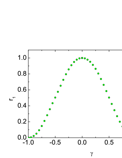
Figure 1: Values of $r_{1}$ found for various $\gamma$’s in such a way that the right hand side of Eq. (46) reproduces the left hand one the most precisely. The maximum $|l_{1}|$ and $|j_{1}|$ were selected to equal $2N=200$.

Then, Eq. (44) contains only “even” or “odd” exponential functions and the constant. Collecting the coefficients at each of those functions, including the constant, equating them to zero, and making some transformations, we obtain the equations

$$b_{0}=-\sum\limits_{p=1,2,\ldots}\frac{a_{p}[g_{p}(-p)+zg_{-p}(p)]}{2\omega n_{0}}\frac{2m}{\hbar^{2}\tilde{k}_{p}^{2}}$$

$$\times[\tilde{E}_{f}^{2}(\tilde{k}_{p},0,\zeta(0,p))-\zeta(0,p)\hbar^{2}\omega^{2}],$$ (48)

$$\sum\limits_{p=1,2,\ldots}a_{p}[g_{p}(j-p)+zg_{-p}(j+p)]$$ (49)

$$\times[\tilde{E}_{f}^{2}(\tilde{k}_{p},k_{j},\zeta(j,p))-\zeta(j,p)\hbar^{2}\omega^{2}]2m/(\hbar^{2}\tilde{k}_{p}^{2})=0,$$

$$\tilde{E}_{f}^{2}(\tilde{k}_{p},k_{j},\zeta)=\zeta\left(\frac{\hbar^{2}\tilde{k}_{p}^{2}}{2m}\right)^{2}+\frac{\hbar^{2}\tilde{k}_{p}^{2}}{2m}n_{0}\nu(k_{j}).$$ (50)

Expression (49) is a system of equations enumerated by the index $j=\pm 1,\pm 2,\ldots$. Equations (48) and (49) take account of symmetry relation (42). If both $j$ and $p$ are either even or odd, then, $\zeta(j,p)=r_{1}$; otherwise, $\zeta(j,p)=r_{2}$. If the sign of $j$ in Eq. (49) changes, either the equation does not change or the sign before the whole equation changes. Therefore, we consider only positive $j$’s.

It is important that, while deriving Eqs. (48)–(50), we collected coefficients before the functions $e^{i2\pi l_{1}x/L}$ and $e^{i\pi(2j_{1}+1)x/L}$ regarded as independent. In fact, they are dependent, but, if the exponential functions $e^{i2\pi l_{1}x/L}$ are expanded in series of $e^{i\pi(2j_{1}+1)x/L}$ or vice versa, the matter is expectedly reduced to a single complete set of functions, and the Bogolyubov dispersion law is obtained for both wave packets (1a) and (1b). However, we may collect coefficients before $e^{i2\pi l_{1}x/L}$ and $e^{i\pi(2j_{1}+1)x/L}$ independently, without expanding either of those functions in the set of the others. If we succeed in zeroing all the coefficients before those functions in Eqs. (13) and (14), the latter will evidently be satisfied, i.e. we will find their solution. The solution of the problem by expanding the function in a complete basis set is a kind of stereotype, and its application is not useful in our case. Since the harmonics are entangled in the integrand of Eq. (14), there emerges a harmonic interplay, which results in that different dispersion laws correspond to wave packets with different structures.

Boundary condition (15) bring about the equation

$$(\tan{\pi\gamma/2})^{z}=z\frac{\sum\limits_{l=1,2,\ldots}a_{2l}\cos{\pi l}}{\sum\limits_{j=0,1,2,\ldots}a_{2j+1}\sin{\pi(j+1/2)}}.$$ (51)

Thus, the coupled equations (49)–(51) are to be solved. This can be done in the following manner. System (49) with an initial $\gamma$-value is solved first. Then, the “theoretical” $\gamma$ is determined from the left hand side of Eq. (51). The initial $\gamma$ is varied from $-1$ to 1, excluding the points $\gamma=-1$ and 0. Those initial $\gamma$’s that coincide with their theoretical counterparts are the sought solutions.

The process is as follows. For a given initial $\gamma$-value, system (49) is solved and the full set of characteristic frequencies is determined. The frequencies are enumerated, starting from the smallest one and ascribing them the numbers $1,2,3,\ldots$. Then, some frequencies are selected (we examined the frequencies with the numbers 1, 2, 8, 9, 29, 30, 49, 50, 99, and 100), and the initial value of $\gamma$ is smoothly varied from $-1$ to 1 for each of them, thus finding solutions for $\gamma$. It turned out that there are several $\gamma$-solutions for the frequency with the given number.

The frequencies are determined as follows. System (49) looks like

$$\sum\limits_{p=1,2,\ldots}a_{p}A_{jp}=0,\ j=1,2,\ldots.$$ (52)

The quantity $\hbar^{2}\omega^{2}$ in the coefficients $A_{jp}$ are taken in form (33) with $k_{0}=\pi j_{0}/L$ and $j_{0}=100$, and $q^{eff}$ is smoothly varied from $-100$ to 1000. At some $q^{eff}$’s, the absolute value of $A_{jp}$-matrix determinant drastically decreases (approximately by two orders of magnitude), and those $q^{eff}$-values are characteristic frequencies, the roots $\hbar^{2}\omega^{2}$ of equation $\mathrm{det}~{}A_{jp}=0$. Dispersion law (34) is found with the help of relation (35). A numerical calculation was made for $N=100$ and $r_{1}$ from Fig. 1. A $2N\times 2N$ matrix was used to represent $A_{jp}$ (the increase of matrix size affected the results very weakly). The interatomic potential was simulated by formula (37) with $U_{0}=0.1~{}\mathrm{K}$ and $a=0.1\bar{R}$. In Figs. 3 and 3, the frequency values are depicted. The coefficient $q$ in dispersion law (34) is close to 1/2 for relatively large $k$’s (for the Bogolyubov solution, $q=1$). For small $k$’s, the magnitude of $q$ is smaller; it differs for different roots and depends on $U_{0}$ and $a/\bar{R}$. Besides, $E$ weakly depends on $\gamma$ and $r_{1}$. Its dependence on $r_{1}$ is associated with the error arising owing to the account of the finite number of summands in expansion (46). The dependence on $\gamma$ is conspicuous at small $k$’s, when the ratio between the fractional, $\pi\gamma/L$, and integer, $\pi j/L$, parts of $k$ is not small.

Figure 2: Dispersion laws: Bogolyubov (3) (rhombs); curve (4), (34) with $q=1/2$ (circles); and numerical solutions of system (49) and (51) at $z=-1$ (crosses). Here, $k_{min}=\pi/L$, $E_{0}=\hbar^{2}k_{m}^{2}/2m$, and $k_{m}=2\pi/\bar{R}$. Hundred ($N=100$) He⁴ atoms with interatomic potential (37) were considered; $U_{0}=0.1~{}\mathrm{K}$ and $a=0.1\bar{R}$.

Figure 3: The same as in Fig. 3, but for large $k$’s.

Note that the network of smallest roots $q^{eff}$ is extremely dense at $j_{0}\gg 1$, so that $q^{eff}$ must be varied with a very short increment for not to miss any root. There are no lost roots if the number of roots equals the number of rows in our square matrix.

As the initial $\gamma$-value varies, the theoretical $\gamma$ obtained from Eq. (51) oscillates with various amplitudes of an order of 1. Often, the period of oscillations is very short, e.g., 10^-6 or even 10^-9. This is possible, because the system of equations is large and strongly nonlinear with respect to $\gamma$. The majority of solutions lie on such small oscillations. The periods of some oscillations are extremely short, so that the corresponding solutions can be easily overlooked. They must be found by feeling, and the procedure of finding them takes a lot of time. Unfortunately, the method does not guarantee that all the solutions have been found. One cannot even say how many solutions exist for every frequency root.

The solutions that we managed to find are depicted in Figs. 3 and 3 by crosses. They determine a dispersion curve lying below the Bogolyubov one. Moreover, we did not obtain a curve but a strip consisting of a good many points (the M-strip, a derivative of “many”). Why did we obtain a strip rather than a curve? This can be 1) a result of zero BCs, 2) owing to the coordinate-momentum uncertainty relation for the quasiparticle, and 3) the strong spread of points can be associated with the fact that the wave packet does not correspond to the solution exactly (instead of one maximum, the packet usually includes two close maxima, see section V).

In order to plot the dispersion curve, one should know the $E$- and $k$-values for every point. The energy can be found unambiguously from the equations, whereas $k=k^{wp}$ is determined from the wave-packet structure, inexactly if $k$ is small (see section V). The energy $E$ is low at small $k$ and is also found inexactly if the determination error $\triangle E\sim E$. Therefore, the nonlinearity of the dispersion curve at small $k$ (see Fig. 3) are connected, most likely, with the calculation error, so that if the calculation were exact, we would obtain the linear law of the type $E=ck$ with $q\approx 1/2$. (According to general theorems yukalov2011 , phonons in the superfluid Bose liquid originates from a spontaneous violation of gauge symmetry and have to possess the asymptotic $E(k\rightarrow 0)=ck$. However, the theorems were proved for periodic BCs, and we do not know whether they remain valid for zero ones.)

Let us return to the general procedure. We solved the linear system of 200 equations (49). For a given $\gamma$, it has 200 solutions for $\omega^{2}$. Plotting the dependences of all 200 frequencies on the initial $\gamma$ in the interval $\gamma\in\left]-1,1\right]$, we obtain a network of 200 lines. Each of them corresponds to a frequency with a certain number. In this network, the lines sometimes intersect each other and break. In the latter case, a new line emerges elsewhere. For every line, there are several points where the initial and theoretical $\gamma$’s coincide. Just those points are the system energy levels. We found solutions only for $z=-1$. If $z=1$, the equations are similar, and so must be their solutions. As a result, the number of levels in the M-strip will be approximately doubled.

For the first (lowest) energy level, we found 2 solutions (we designate this as $1_{2}$), and for the next levels $2_{2}$, $8_{3}$, $9_{9}$, $29_{5}$, $30_{8}$, $49_{7}$, $50_{3}$, $99_{16}$, and $100_{13}$. They are shown in Figs. 3 and 3. For every frequency solution, we solved Eq. (49) to find the coefficients $a_{p}$ for wave packet (2b) (Eq. (21)). As a rule, the packet included two closely located maxima (see Fig. 4), over which we determined by eye the $p$-index value corresponding to the packet center and found the packet wave vector $\tilde{k}_{p}=\pi(p+\gamma(p))/L$. Some packets had 1 or 3 maxima. Those $\tilde{k}_{p}$’s were substituted as $k$ into the dispersion law $E(k)$.

The main result of this section consists in that wave packets (2a) and (2b) are characterized by a new dispersion law (34) with $q\approx 1/2$.

V Solution structure

In sections II and III, we found that the Bogolyubov dispersion law corresponds to solutions (1a) with $\gamma=\pm 1/2$ and (1b) with $\gamma=0$. The packet wave vector $k^{wp}=2\pi(l_{0}+\gamma)/L>0$. The structure of packet (1a) was found by substituting the solution for $\omega$ with the $j$-th number into Eq. (31) and solving the latter with respect to the coefficients $a_{2l}$. The coefficient $a_{2l}$ with $l=j$ turned out the largest one, the neighbor coefficients $a_{2l}$ (with $l=j\pm 1$) were less by 2 to 3 orders of magnitude, and the next coefficients were even less. It means that the packet is strongly localized in the $k$-space, as well as packet (1b) zero-gas2 . Therefore, it is easy to find the value $k=k^{wp}$ for the dispersion law $E(k)$: we should use in the formula $k^{wp}=2\pi(l_{0}+\gamma)/L$ the number $l_{0}=j$ of the largest $a_{2j}$.

For the M-mode (Figs. 3 and 3), the situation is much more complicated. The basic issues are: What is the nature of this solution? Is it a new oscillatory mode or a superposition of several Bogolyubov modes? The formula for the wave packet reads

$$\tilde{n}(x,k^{wp})=2\sum\limits_{l=1,2,\ldots}a_{2l}(l_{0})\sin{[\pi(2l+\gamma)x/L]}$$

$$+2\sum\limits_{j=0,1,2,\ldots}a_{2j+1}(l_{0})\sin{[\pi(2j+1+\gamma)x/L]}$$

$$=\sum\limits_{l=\pm 1,\ldots}a_{2l}e^{i\pi(2l+\gamma(2l))x/L}$$

$$+\sum\limits_{j=0,\pm 1,\ldots}a_{2j+1}e^{i\pi(2j+1+\gamma(2j+1))x/L}.$$ (53)

It should be appended by Eqs. (41), (42), $z=-1$, and by BC (51). Harmonics with odd numbers can be expanded in harmonics with even numbers, i.e. in the Fourier series,

$$e^{i\pi(2j+1)x/L}=\frac{2}{\pi}\sum\limits_{p}\frac{\sin{[\pi(2p-2j-1)/2]}}{2p-2j-1}e^{i\pi 2px/L},$$

where $p$’s are integers. Then, wave packet (53) looks like

$$\tilde{n}=2\sum\limits_{l=0,1,2,\ldots}\tilde{a}_{2l}(l_{0})\sin{[\pi(2l+\gamma)x/L]}$$

$$+2\sum\limits_{l=1,2,\ldots}\tilde{c}_{2l}(l_{0})\sin{[\pi(2l-\gamma)x/L]},$$ (54)

i.e. it is a sum of two packets with “even” harmonics, where $\gamma$ is left as a quantum number. For every “even” packet, the Bogolyubov dispersion law is valid, but the zero BC is not obeyed. If the zero BC has been satisfied for each of those packets at any frequency, packet (53) would have been a sum of two or more Bogolyubov packets. However, the zero BC is obeyed only for the whole sum (53); therefore, the M-mode is not reduced to a sum of several solutions of the Bogolyubov type. Hence, this is a new solution. The fact that it is constructed on the basis of two basis sets makes the solution less clear and a little debatable. However, it seems that the packet center $k_{wp}$ and the dispersion law $E(k)$ can be indicated for the new mode, at least if $k_{wp}$’s are not small.

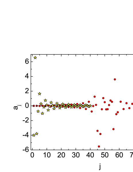
Figure 4: The set of coefficients $a_{j}$ for wave packet (53). The solutions of system (49) and (51) with $z=-1$ are considered for the frequency No. 1 with $E\approx 0.000142E_{0}$, $\gamma\approx 0.6435$, and $k^{wp}\approx 2.64\pi/L$ (stars), and for frequency No. 50 with $E\approx 0.0782E_{0}$, $\gamma\approx-0.6065$, and $k^{wp}=\pi(j^{wp}+\gamma)/L\approx 50.64\pi/L$ (circles; the absolute values of $a_{j}$’s are decreased by a factor of 30). Hundred ($N=100$) He⁴ atoms with interatomic potential (37) were considered; $U_{0}=0.1~{}\mathrm{K}$ and $a=0.1\bar{R}$.

Let us consider the structure of packet (53). For every $\omega$, the coefficients $a_{j}$ are determined from system (49) after substituting the solution for $\omega$ into it. One can see from the results (Fig. 4) that the packet is not strongly localized in the $k$-space. However, the $k^{wp}$-value can be approximately calculated. At large $k^{wp}$, the wave packet includes two close maxima, so that $k^{wp}$ can be evaluated as a half-sum of maximum $k$-values (if either of the maxima is larger, $k^{wp}$ is shifted proportionally). The error obtained for $k^{wp}$ in this case is small, and the value of $E$ for the packet is uniquely determined from the system of equations. Therefore, at large $k^{wp}$, M-packet (53) rather adequately describes the quasiparticle. At small $k^{wp}$, the wave packet has one or two, not very narrow, maxima, the $k$-values of which slightly exceed the increment step of $k$. In this case, the value of $k^{wp}$ is determined unreliably. Most likely, the dispersion curve (Fig. 3) has a “dip”  because small $k^{wp}$’s were determined inaccurately. Perhaps, there may exist another representation of packet (53) as a sum of harmonics, for which the wave packet has a single sharp maximum at small $k^{wp}$. If we associate $k^{wp}$ with this maximum, the dispersion law should probably be of the linear type, $E=ck$. However, we did not find such a representation.

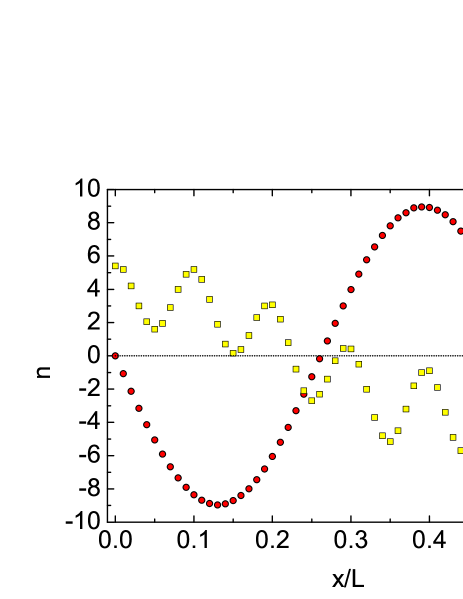
Figure 5: Dependence $\tilde{n}(x)$ for new mode (53) for one of the solutions for the 9-th (circles) and 30-th (squares) frequencies. For the 9-th frequency, $E\approx 0.005E_{0}$, $\gamma\approx-0.1$, and $k^{wp}\approx 8.9\pi/L$; and for the 30-th one, $E\approx 0.036E_{0}$, $\gamma\approx 0.64$, and $k^{wp}\approx 31.64\pi/L$L. Hundred ($N=100$) He⁴ atoms with interatomic potential (37) were considered; $U_{0}=0.1~{}\mathrm{K}$ and $a=0.1\bar{R}$. For illustrative purposes, the curve for the 30-th frequency is stretched tenfold along the $x$-axis, so that $x=0.5L$ in the figure corresponds to the real $x=0.5L$, and $x=0$ in the figure to real $x=0.45L$.

It is of interest that, in a more exact approach zero-liquid , the solution for the phonon is so constructed that the phonon is described by a single harmonic rather than a wave packet. As a result, $k$ is determined unambiguously. In this case, $E(k\rightarrow 0)=ck$.

Figure 5 illustrates solution (53) in the $x$-space (for two arbitrary $E$-roots). The curve composed by squares looks rather strange. This density distribution is probably unstable. Notice that, at small $k^{wp}=\pi(l_{0}+\gamma)/L$, the number of zeros for the function $\tilde{n}(x)$ is considerably less than that for $\sin{k^{wp}x}$, with those two numbers getting closer as ${k^{wp}}$ grows.

VI Thermodynamics

According to the analysis given above, the following points correspond to the Bogolyubov curve: one $\omega$ for every $k=2l\pi/L$, two very close $\omega$’s for every $k=(2l+1)\pi/L$ ($l=1,2,\ldots$), and one $\omega$ for $k=\pi/L$. We may average over the nearest levels and consider that any interval $\triangle k=\pi/L$ includes $\alpha(k)=1.5$ points. The free energy of the system equals land5

$$F=-k_{B}T\ln\sum\limits_{n}e^{-E_{n}/k_{B}T}.$$ (55)

In our case,

$$F=-k_{B}T\ln{\left(\sum\limits_{k=\pi j/L>0}\alpha(k)e^{-E_{k}/k_{B}T}\right)}.$$ (56)

For the Bogolyubov curve, $\alpha(k)$ does not depend on $k$ and leads only to the summand $-k_{B}T\ln\alpha$. It is unobservable, because it changes the system entropy $S=-\partial F/\partial T$ but not the total energy $E=F+TS$ and the heat capacity $C=T\partial S/\partial T$.

The M-strip gives its contribution to $F$. According to available data, $\alpha(k)\sim 5$ for frequencies with numbers $1$-$5$, and $\alpha(k)\sim 10$ for frequencies with numbers $\gtrsim 10$. Moreover, $\alpha$ chaotically changes when passing to next levels. No evident growth or decrease of $\alpha$ was observed as $k$ grew.

VII Comparison with experiment

We found two possible dispersion laws for the uniform 1D Bose gas in a box: the Bogolyubov law and a new one (4) with $q=1/2$. A similar problem was solved for the $f$-dimensional case using a more exact method zero-liquid , and dispersion law (4) with $q=2^{-f}$ was obtained. Unlike the GP method, the approach zero-liquid catches the structure of the system ground state. In this approach, different ground states (with different energies $E_{0}$) correspond to the Bogolyubov and new dispersion laws. Therefore, the system should be so ordered that either all phonons obey the Bogolyubov dispersion law or they have dispersion law (4) with $q=2^{-f}$. In the 2D and 3D cases, $E_{0}$ is lower for the new solution zero-liquid ; therefore, it has to be realized in the Nature, whereas the Bogolyubov ordering should be unstable.

How can all that be verified experimentally? The dispersion law should be measured for the uniform Bose gas, with boundaries and cyclic, and the results should be compared. A cyclic system of any dimensionality is characterized by the Bogolyubov dispersion law only. As far as we know, uniform 1D systems have not been created yet. A three-dimensional system cannot be made closed. However, such an experiment is quite possible for 2D films; and this is probably the main way of verification zero-liquid .

A huge number of experiments are carried out now with gases in traps, but they seem not to be useful in verifying the effect. The reason is as follows. In the case of uniform system, when changing from periodic BCs to zero ones, the second dispersion law manifests itself owing to the interaction between the harmonics in the potential expansion and the harmonics in the expansion of density oscillations in the integral in the Gross equation. Gas in a trap is a cloud, which is dense near the center. At a distance of about the Thomas-Fermi length from the center, the concentration becomes low and rapidly decreases further. The cloud is in a vessel, the size of which is much larger than the Thomas-Fermi length; therefore, the gas atoms are practically absent near the vessel walls. For this system, oscillatory functions are characteristic ones. If the system becomes closed in the region of boundaries, oscillatory functions change only in this region. However, both the concentration and the low-order oscillatory functions are small there; therefore, the integral in the Gross equation must be almost identical under zero and periodic BCs. Accordingly, the dispersion laws must also be close to each other. If the system is uniform, the characteristic functions are plane waves (not small in the whole space), and the change from periodic to zero BCs manifests itself in Eq. (23) as the increment modification, $\triangle k=2\pi/L\rightarrow\pi/L$, and a factor of 1/2 before $\nu(k)$. As a result, the integral in the Gross equation brings about different solutions for periodic and zero BCs.

For gases in the trap, the integral in the Gross equation does not feel the difference between the topologies of closed and open systems. Therefore, it can be calculated approximately, assuming the potential to be point-like and thus changing to the GP equation. This is an ordinary way. The GP equation leads to the Bogolyubov formula for the dispersion law in a uniform system. This circumstance favors the application of this formula rather than Eq. (4) as the basic dispersion law in the local density approximation (LDA). In the work by Stringari stringari1996 , the low-lying 3D levels were calculated from the GP equation, and they agreed with the experiment cornell1996 ; ketterle1996 ; ketterle2000 . For a 1D gas in the trap, experimentally measured lower levels esslinger2003 ; nagerl2009 approximately agree with theoretical ones stringari2002 ; santos2003 ; superTG . For the linear and square-law regions in the dispersion curve in the 3D geometry, the theory (zaremba1998 ; tozzo2003 and LDA) approximately agrees with the experiment for ²³Na ketterleE1 ; ketterle1999 ; ketterleE2 and ⁸⁷Rb steinhauer2002 ; steinhauer2003 ; steinhauer2012 atoms (see also review ozeri2005 ).

Notice that, in the often used LDA, the dispersion law for a localized wave packet in a non-uniform medium is assumed zambelli2000 to be the same as for a packet in an infinite uniform environment of the same density. However, the localized packet is a superposition of nonlocal modes; therefore, the dispersion law for the packet can turn out a nonlocal property. For today, there is no clear evidence that this is so, but the rigorous substantiation of LDA is also absent. The accuracy of LDA can be elucidated by constructing a wave packet on the basis of exact solutions for nonlocal modes of non-uniform system.

VIII Conclusions

In this work, we tried to find a dispersion law for the one-dimensional uniform Bose gas under zero boundary conditions. We proceeded from the Gross equation (2) making allowance for the non-point character of interaction. Two solutions were found: the known Bogolyubov dispersion curve (which is reproduced with a high accuracy) and a new curve $E(k)$ that lies below the Bogolyubov one. The new curve can be reliably determined at large $k$’s and not so reliably at small $k$’s. It agrees well with a solution for $E(k)$ found by a different method zero-liquid for a one-, two-, and three-dimensional systems. The stability of solutions was not analyzed. Which of two dispersion laws is realized in experiment can be elucidated by studying homogeneous rarefied He II films zero-liquid .

An actual non-point potential is replaced by the point-like one, because the former is very complicated and is not known precisely, whereas the latter simplifies the equations very much. As far as we understand, this replacement is justified for the description of atomic scattering. However, for studying the collective properties of Bose gas at $T\rightarrow 0$, it is not justified, since the new solution becomes lost. Collective oscillations and Fourier components of potential are modulated by the walls zero-liquid , and they mutually interact in the integral in the Gross equation. If the non-point character of interaction is taken into account, the Fourier components strongly change, and a new solution for collective modes emerges.

The problem of an influence of boundaries is interesting but not simple. To make this issue clear, unbiased researches using various theoretical methods and special experiments are required. We hope that this work will be useful.

References

- (1) M. Girardeau, J. Math. Phys. (N.Y.) 1, 516 (1960).
- (2) E.H. Lieb, W. Liniger, Phys. Rev. 130, 1605 (1963); E.H. Lieb, Phys. Rev. 130, 1616 (1963).
- (3) M. Gaudin, Phys. Rev. A 4, 386 (1971).
- (4) C. Menotti and S. Stringari, Phys. Rev. A 66, 043610 (2002).
- (5) P. Pedri and L. Santos, Phys. Rev. Lett. 91, 110401 (2003).
- (6) G.E. Astrakharchik, J. Boronat, J. Casulleras, and S. Giorgini, Phys. Rev. Lett. 95, 190407 (2005).
- (7) H. Moritz, T. Stöferle, M. Köhl, and T. Esslinger, Phys. Rev. Lett. 91, 250402 (2003).
- (8) E. Haller, M. Gustavsson, M.J. Mark, J.G. Danzl, R. Hart, G. Pupillo, and H.-C. Nägerl, Science 325, 1224 (2009).
- (9) L.P. Pitaevskii, Sov. Phys. JETP 13, 451 (1961).
- (10) E.P. Gross, J. Math. Phys. 4, 195 (1963).
- (11) E.P. Gross, Phys. Rev. 106, 161 (1957).
- (12) M.D. Tomchenko, Ukr. J. Phys. 59, 123 (2014); arXiv:cond-mat/1201.1845.
- (13) N.N. Bogoliubov, J. Phys. USSR 11, 23 (1947).
- (14) N.N. Bogolyubov and D.N. Zubarev, Sov. Phys. JETP 1, 83 (1956).
- (15) M. Tomchenko, arXiv:cond-mat/1211.1723.
- (16) N.J. van Druten and W. Ketterle, Phys. Rev. Lett. 79, 549 (1997).
- (17) M.D. Girardeau, E.M. Wright, and J.M. Triscari, Phys. Rev. A 63, 033601 (2001).
- (18) D.S. Petrov, D.M. Gangardt, and G.V. Shlyapnikov, J. Phys. IV France 116, 5 (2004); arXiv:cond-mat/0409230.
- (19) C.J. Pethick, H. Smith, Bose-Einstein Condensation In Dilute Gases (Cambridge University Press, New York, 2008).
- (20) M.D. Tomchenko, arXiv:cond-mat/1403.8014.
- (21) V.I. Yukalov, Phys. Part. Nucl. 42, 460 (2011).
- (22) L.D. Landau and E.M. Lifshitz, Statistical Physics, 3rd ed., Part 1, (Pergamon Press, Oxford, 1980; Nauka, Moscow, 1976).
- (23) S. Stringari, Phys. Rev. Lett. 77, 2360 (1996).
- (24) D.S. Jin, J.R. Ensher, M.R. Matthews, C.E. Wieman, and E.A. Cornell, Phys. Rev. Lett. 77 420 (1996).
- (25) M.-O. Mewes, M.R. Andrews, N.J. van Druten, D.M. Kurn, D.S. Durfee, C.G. Townsend and W. Ketterle, Phys. Rev. Lett. 77 988 (1996).
- (26) R. Onofrio, D.S. Durfee, C. Raman, M. Köhl, C.E. Kuklewicz, and W. Ketterle, Phys. Rev. Lett. 84 810 (2000).
- (27) E. Zaremba, Phys. Rev. A 57, 518 (1998).
- (28) C. Tozzo and F. Dalfovo, New J. Phys. 5, 54 (2003).
- (29) M.R. Andrews, D.M. Kurn, H.-J. Miesner, D.S. Durfee, C.G. Townsend, S. Inouye, and W. Ketterle, Phys. Rev. Lett. 79, 553 (1997); M.R. Andrews, D.M. Stamper-Kurn, H.-J. Miesner, D.S. Durfee, C.G. Townsend, S. Inouye, and W. Ketterle, Phys. Rev. Lett. 80, 2967 (E) (1998).
- (30) D.M. Stamper-Kurn, A.P. Chikkatur, A. Görlitz, S. Inouye, S. Gupta, D.E. Pritchard, and W. Ketterle, Phys. Rev. Lett. 83, 2876 (1999).
- (31) J. Stenger, S. Inouye, A.P. Chikkatur, D.M. Stamper-Kurn, D.E. Pritchard, and W. Ketterle, Phys. Rev. Lett. 82, 4569 (1999).
- (32) J. Steinhauer, R. Ozeri, N. Katz, and N. Davidson, Phys. Rev. Lett. 88, 120407 (2002).
- (33) J. Steinhauer, N. Katz, R. Ozeri, N. Davidson, C. Tozzo, and F. Dalfovo, Phys. Rev. Lett. 90, 060404 (2003).
- (34) I. Shammass, S. Rinott, A. Berkovitz, R. Schley, and J. Steinhauer, Phys. Rev. Lett. 109, 195301 (2012).
- (35) R. Ozeri, N. Katz, J. Steinhauer, and N. Davidson, Rev. Mod. Phys. 77,187 (2005).
- (36) F. Zambelli, L. Pitaevskii, D.M. Stamper-Kurn, and S. Stringari, Phys. Rev. A 61, 063608 (2000).