Exact non-equilibrium solutions of the Boltzmann equation under a time-dependent external force

Abstract

We construct a novel class of exact solutions to the Boltzmann equation, in both its classical and quantum formulation, for arbitrary collision laws. When the system is subjected to a specific external forcing, the precise form of which is worked out, non equilibrium damping-less solutions are admissible. They do not contradict the $H$-theorem, but are constructed from its requirements. Interestingly, these solutions hold for time-dependent confinement. We exploit them, in a reverse-engineering perspective, to work out a protocol that shortcuts any adiabatic transformation between two equilibrium states in an arbitrarily short time-span, for an interacting system. Particle simulations of the direct Monte Carlo type fully corroborate the analytical predictions.

More than 140 years after its derivation by J. Maxwell Maxwell and L. Boltzmann Boltzmann1872 , the so-called Boltzmann equation has kept the essence of its original formulation, its predictive power and its interest. It lies at the heart of the theory of transport in solids, energy transfer in plasmas, space shuttle aerodynamics, complex flows in micro-electromechanical systems, neutron transport in nuclear reactors, or granular gas dynamics, to name but a few relevant applications in non equilibrium statistical physics Cercignani ; Kremer . It moreover gradually became a thriving branch of mathematics, particularly active in the last 20 years, see e.g. Villani02 ; SaintRaymond and references therein. The Boltzmann equation applies to systems that are rarefied in some sense, such as an ultracold gas which provides an appropriate setting to illustrate the forthcoming discussion pethick1 ; david99 ; pethick2 ; quadupolemonopole0 ; quadupolemonopole1 ; quadupolemonopole2 .

Working on kinetic theory circa 1870 was a leap of faith, impeded by the controversy pertaining to the atomic nature of matter. It is a great triumph of Boltzmann to have derived the $H$-theorem, showing that the system under scrutiny evolves towards equilibrium, thereby bridging microscopic dynamics and macroscopic irreversibility. To this end, a Lyapunov function was constructed, a non-increasing functional of the probability distribution function $f({\boldsymbol{r}},{\boldsymbol{v}},t)$ for finding gas molecules at position ${\boldsymbol{r}}$ with velocity ${\boldsymbol{v}}$ at a given time $t$. It was historically the first Lyapunov function, and it attributed a direction in time to the Boltzmann equation. A consequence of the $H$-theorem is that at long times, $\log f$ is a collisional invariant, which as such should exhaust all independently conserved quantities (momentum, energy in addition to a trivial yet relevant constant), so that for like-mass molecules, $\log f$ should be a linear combination of 1, $\boldsymbol{v}$ and $v^{2}$:

$$f({\boldsymbol{r}},{\boldsymbol{v}},t)\,=\,\exp\left\{-\alpha-\beta v^{2}-{\boldsymbol{\gamma}}\cdot{\boldsymbol{v}}\right\}.$$ (1)

In all generality, $\alpha$, $\beta$ and $\boldsymbol{\gamma}$ are both position and time dependent, with the constraint $\beta>0$ comment3 . The well known Maxwell-Boltzmann Gaussian form with constant (say vanishing) $\boldsymbol{\gamma}$ and a constant inverse temperature $\beta$ is a particular solution. Less known, but nevertheless recognized by Boltzmann himself Boltzmann ; Cercignani is the fact that more exotic solutions could exist under harmonic confinement, that are still of the form (1) but with a time dependent kinetic temperature $\propto\beta^{-1}$. These solutions can be envisioned as breathing modes, where a perpetual conversion of kinetic and potential energy operates through a swing-like mechanism and it is essential here that the coupling term $\boldsymbol{\gamma}$ be position and time dependent. Another remarkable feature of the breathing mode is that it is not restricted to small amplitude oscillations. These somewhat non standard solutions were hitherto considered as a side curiosity, a point of view epitomized by Uhlenbeck, who wrote “…for special outside potentials for instance the harmonic potential $U(r)=\omega r^{2}/2$ the spatial equilibrium distribution will not be reached in time. For such special potentials there are a host of special solutions of the Boltzmann equation (…) where the (coefficients) can be functions of space and time. (…) They have however only a limited interest” Uhl63 . Uhlenbeck’s statement applies to static confinement; It is our goal here to show the possibility of generalized breathing modes for time-dependent forcing, and to make use of these modes to propose a new kind of gas manipulation on a timescale much shorter than the one dictated by the thermodynamical adiabaticity criterion. In doing so, we put forward a reverse engineering perspective, opposed to the direct approach of Uhlenbeck, and applying in the quantum realm as well. Similar protocols have recently been dubbed ‘shortcuts to adiabaticity’ Chen1 ; reviewsta in quantum systems comment , and brought to bear in the realm of transport TransportDavid , wave-packet splitting or internal state control of single atoms, ions, or Bose-Einstein condensates and other many-body systems Adol . However, in contrast with other phase space manipulation techniques such as the Delta Kick Cooling deltakick , the method proposed here is operational for interacting systems and on an arbitrary short time scale. As a byproduct of the analysis, we uncover for static confinement new particular potentials allowing for the perpetual non equilibrium solutions of the form (1). Surprisingly, these solutions were missed by Boltzmann, an omission that propagated ever since in the literature.

The Boltzmann equation hinges on a low density prerequisite which dramatically simplifies the exact $N$-body dynamics into a non-linear integro-differential equation for the single particle distribution $f({\boldsymbol{r}},{\boldsymbol{v}},t)$. Its rate of change stems from two effects, free streaming and binary collisions, which translate into the balance equation Cercignani ; Kremer

$$\left(\partial_{t}\,+\,{\boldsymbol{v}}\!\cdot\!{\boldsymbol{\nabla}}_{\boldsymbol{r}}+{\boldsymbol{F}}({\boldsymbol{r}},t)\!\cdot\!{\boldsymbol{\nabla}}_{\boldsymbol{v}}\right)f\,=\,I_{\text{coll}}[{\boldsymbol{v}}|f,f],$$ (2)

where the external (trap) force $\boldsymbol{F}({\boldsymbol{r}},t)$ denotes a position and time-dependent field that will be considered conservative: $\boldsymbol{F}=-{\boldsymbol{\nabla}}_{\boldsymbol{r}}V$. For simplicity, we assume that all molecules have the same (unit) mass. The collisional integral $I_{\text{coll}}$ is a bilinear operator acting on $f$, which depends on the precise form of scattering law considered. We shall not need to specify it further since all solutions inspected will be of the form (1) and by virtue of the $H$-theorem, they identically nullify $I_{\text{coll}}$. It is straightforward to check that the equilibrium barometric law $f\propto\exp(-2\beta V-\beta v^{2})$ is a solution for the Boltzmann equation (2). As alluded to above, Boltzmann realized that for a harmonic static trap ($V\propto r^{2}$), more general oscillating solutions of the form (1) were admissible Boltzmann . In repeating his argument, subsequent authors systematically missed other forms of confinement that turn out to be compatible with a breathing behavior. Our goal is however more general than correcting for that shortcoming, and and we will explore the venue opened by a suitably chosen time-dependent trapping, a so far untouched question. To this end, we introduce relation (1) into (2), which leads to

$${\boldsymbol{\nabla}_{\boldsymbol{r}}}\,\beta\,=\,\boldsymbol{0},$$ (3)

$$v^{2}\partial_{t}\beta+{\boldsymbol{v}}\cdot\!{\boldsymbol{\nabla}_{\boldsymbol{r}}}(\boldsymbol{\gamma}\cdot\!\boldsymbol{v})\,=\,0,\quad\hbox{for all }\boldsymbol{v},$$ (4)

$$\partial_{t}\boldsymbol{\gamma}+\boldsymbol{\nabla}_{\boldsymbol{r}}\,\alpha+2\beta\boldsymbol{F}\,=\,\boldsymbol{0},$$ (5)

$$\partial_{t}\alpha+\boldsymbol{F}\cdot\boldsymbol{\gamma}\,=\,0.$$ (6)

Any triplet ($\alpha$, $\beta$, $\boldsymbol{\gamma}$) fulfilling Eqs. (3)-(6) is a solution to Eq. (2), and we of course recover the barometric law ($\alpha=2\beta V$, $\beta$ uniform and constant, $\boldsymbol{\gamma}=\boldsymbol{0}$) among all possible solutions.

The structure of the system (3)-(6) constrains the possible form of $\boldsymbol{F}=-\boldsymbol{\nabla}_{\boldsymbol{r}}V$, a feature which we now analyze. We learn from Eqs. (3) that $\beta$ is a sole function of time. In addition, the general solution of (4) can be written

$$\boldsymbol{\gamma}(\boldsymbol{r},t)\,=\,\boldsymbol{\gamma}_{0}(t)\,+\,\boldsymbol{J}\wedge\boldsymbol{r}\,-\,\dot{\beta}\,\boldsymbol{r},$$ (7)

where the dot denotes time derivation. Equation (5) implies that $\partial_{t}\,(\hbox{\bf curl}\,{\boldsymbol{\gamma}})=\boldsymbol{0}$ which supplemented with $\hbox{\bf curl}\,\boldsymbol{\gamma}=\boldsymbol{J}$ [see Eq. (7)], imposes that $\boldsymbol{J}$ be constant and uniform. It can be shown that $\boldsymbol{J}$ corresponds to the total angular momentum of the system, a conserved quantity. In what follows, we will put $\boldsymbol{\gamma}_{0}(t)=\boldsymbol{0}$ which is always possible up to an innocuous shift of the velocity origin comment2 . We focus for simplicity on vanishing angular momentum solutions, which display already the most interesting properties. The case $\boldsymbol{J}\neq\boldsymbol{0}$ is treated in the supplemental material suppl . Combining Eqs. (5), (6) and (7), we arrive at

$$\dot{\beta}\,\left(2+\boldsymbol{r}\cdot\!\boldsymbol{\nabla}_{\boldsymbol{r}}\right)\,V(\boldsymbol{r})\,+\,\,2\beta\,\frac{\partial V}{\partial t}\,+\,\dddot{\beta}\,\frac{r^{2}}{2}\,=\,0,$$ (8)

up to an irrelevant time dependent function, which can be absorbed into $V$ without changing the resulting force $\boldsymbol{F}$. The general solution with $\dot{\beta}\neq 0$ reads

$$V(\boldsymbol{r})=\frac{1}{2}\omega^{2}(t)r^{2}+\frac{b}{r^{2}},$$ (9a)

with $$\dddot{\beta}+4\omega^{2}\dot{\beta}\,+\,4\,\omega\,\dot{\omega}\,\beta\,=\,0.$$ (9b)

Before discussing the possibilities opened by this class of solutions, a few words are in order on the static confinement case ($\dot{\omega}=0$), where it is seen that the breathing mode obeying $\dddot{\beta}+4\omega^{2}\dot{\beta}=0$ has characteristic frequency $2\omega$, twice the trap frequency. Notably, this mode is unaffected by the non harmonic term in $b/r^{2}$ (here $b\geq 0$ for normalizability). While the harmonic solution with $b=0$ has been known since the 1870s, the more general form with $b\neq 0$ has ben overlooked, and provides a new family of exact solutions to the Boltzmann equation.

For a general time-dependent confinement ($\dot{\omega}\neq 0$), Eq. (9b) gives the evolution of the effective temperature $T(t)\propto\beta^{-1}$ rque50 for a given driving of the trap angular frequency, whatever the collision rate. The evolution of this effective temperature is deeply connected to single particle dynamics, which allows for the possibility of a parametric resonance (not shown). In the remainder however, we focus on an inverse perspective: instead of working out the consequences on dynamical quantities of a given trap driving $\omega(t)$, we first put forward a desired dynamics for $\beta(t)$, and find out the required driving in a second step. This strategy is put to work to perform on a short time scale the same task as an adiabatic transformation, which connects two equilibrium states but requires a slow protocol. Our scheme, which therefore qualifies as a ‘shortcut to adiabaticity’, can be illustrated on the harmonic case ($b=0$), to which we will restrict. It nevertheless also applies for non harmonic trapping with $b>0$. The idea is to first shape the effective temperature to obey a set of boundary conditions, and to design the angular frequency correspondingly. In the absence of elastic collisions, an adiabatic change of the strength of confinement obeys the criterion $|\dot{\omega}|\ll\omega^{2}$, that results from the invariance of the one-particle action LiL92 , and $E/\omega$, where $E$ is the total mechanical energy, remains constant. If elastic collisions are at work, the thermodynamical adiabaticity criterion reads $|\dot{\omega}|/\omega\ll\tau_{\rm relax}^{-1}$, where $\tau_{\rm relax}$ is the relaxation time needed for the gas to recover equilibrium. Under this condition, the population of each single state remains constant as a function of time, and therefore the quantity $T/\omega$ remains constant. The relaxation time depends on the relative value between the mean free time $\tau$ and the oscillation period $2\pi/\omega$ relax ; comment4 .

Such an adiabatic evolution can be here easily recovered from Eq. (9b) by dropping the $\dddot{\beta}$ term, which yields $\beta(t)\omega(t)=\beta(0)\omega(0)$. For this slow evolution, the position-velocity correlation scaling function $\boldsymbol{\gamma}$ vanishes (again, up to a possible rigid rotation). As demonstrated below, the previously found solutions enable us to generalize the concept of shortcut to adiabaticity (STA) for expansions and compressions of a classical gas in a potential of the form (9a). Fast harmonic trap expansions without final excitation were designed for single quantum particles using Lewis-Riesenfeldt invariants Chen1 , and for Bose-Einstein condensates using a self-similar ansatz stabec . These expansions have been already successfully implemented with non-interacting thermal atoms and for Bose-Einstein condensates in the Thomas-Fermi regime Nice1 ; Nice2 .

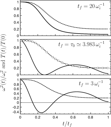
Figure 1: Inverse engineered trap angular frequency as a function of time for a decompression $T_{f}/T_{i}=1/5=\beta_{i}/\beta_{f}$ on three different timescales $t_{f}$ (solid line) and the corresponding time evolution of the effective temperature $\beta_{i}/\beta(s)$ (dashed line), where $\beta(s)$ is given given by Eq. (10). As explained in the main text, above the critical value $t_{f}>\tau_{0}\simeq 3.983\,\omega_{i}^{-1}$ $\omega^{2}$ is always positive (confining potential) whereas for $t_{f}<\tau_{0}$, the trap should necessarily be expulsive ($\omega^{2}<0$) in some intermediate time window. For the critical case $t_{f}=\tau_{0}$, the square symbols display the temperature measured in Monte Carlo simulations of a hard disks system, subject to the confining time-dependent STA harmonic forcing in $\omega(t)$. They are in excellent agreement with the desired behavior embodied in Eq. (10), and shown by the dashed line. A similar agreement with Monte Carlo is found for all transformation times $t_{f}$.

A remarkable feature of the protocol proposed here for the classical gas is that we can relate two equilibrium states whatever the relaxation time of the system is. Let us label the initial and final states by $i$ and $f$ respectively: $\beta_{i,f}=1/(2k_{B}T_{i,f})$ and $\boldsymbol{\gamma}_{i,f}=\boldsymbol{0}$. We assume that these states can be related by an adiabatic transformation so that $T_{i}/\omega_{i}=T_{f}/\omega_{f}$. To shape the time dependence of the trap strength and go from one state to the other in an arbitrary time duration $t_{f}$, we search for a polynomial form of $\beta(t)$ that obeys the boundary conditions selfcons : $\beta(0)=\beta_{i}$, $\dot{\beta}(0)=0$, $\ddot{\beta}(0)=0$, $\dddot{\beta}(0)=0$, $\beta(t_{f})=\beta_{f}$, $\dot{\beta}(t_{f})=0$, $\ddot{\beta}(t_{f})=0$, and $\dddot{\beta}(t_{f})=0$. We find

$$\beta(s)=(\beta_{f}-\beta_{i})(-20s^{7}+70s^{6}-84s^{5}+35s^{4})+\beta_{i},$$ (10)

with $s=t/t_{f}$, that varies monotonously from $\beta_{i}$ to $\beta_{f}$. Once $\beta(t)$ is known, a first order equation on $\omega^{2}$ (see Eq. (9b)) remains to be solved with the boundary condition $\omega^{2}(0)=\omega_{i}^{2}$. From Eq. (9b), we can deduce more on matching conditions: $\dot{\omega}(0)=\dot{\omega}(t_{f})=0$. Self-consistency also implies that $\omega(t_{f})=\omega_{f}$ selfcons . During the evolution, the ratio $T/\omega$ departs from its initial and final values, measuring the deviation from adiabaticity.

As an example, consider a decompression ($\omega_{f}/\omega_{i}<1$). On short timescales, a non monotonous variation of $\omega(t)$ is required to fulfill the boundary conditions. This occurs with our ansatz for $t_{f}<5.904/\omega_{i}$ when $\omega_{f}/\omega_{i}=1/5$. Furthermore, there exists generically a critical time $\tau_{0}$ for the process duration $t_{f}$ below which $\omega^{2}(t)$ is negative during some time interval (i.e. the potential becomes transiently expulsive, in order to speed up the transformation). For our ansatz and boundary conditions ($\omega_{f}/\omega_{i}=1/5$), $\tau_{0}\simeq 3.983/\omega_{i}$. Figure 1 shows the inverse engineered angular frequency, $\omega(t)$, for the three situations $t_{f}>\tau_{0}$, $t_{f}=\tau_{0}$ and $t_{f}<\tau_{0}$. In the case where $T_{f}>T_{i}$ (compression), a very similar phenomenology is observed. In the slow, adiabatic limit $t_{f}\to\infty$, we recover an evolution with $T\propto\omega$, as it should.

To gain more insight into the transient dynamics, it is instructive to study the scaling properties of $f(\boldsymbol{r},\boldsymbol{v},t)$. It can be noted that $\beta^{-1/2}$ sets the relevant velocity scale and that conversely $\beta^{1/2}$ measures the pertinent length scale. The fact that the product of both is in $\beta^{0}$, time independent, can be viewed as a byproduct of angular momentum conservation. Then, rescaling velocities with respect to the local center-of-mass velocity [$-\boldsymbol{\gamma}/(2\beta)$, which is position and time dependent], and defining

$$\widetilde{\boldsymbol{v}}=\sqrt{\beta}{\boldsymbol{v}}+\frac{\boldsymbol{\gamma}}{2\sqrt{\beta}},\quad\widetilde{\boldsymbol{r}}=\frac{\boldsymbol{r}}{\sqrt{\beta}},$$ (11)

the joint distribution of rescaled coordinates $\widetilde{f}(\widetilde{\boldsymbol{r}},\widetilde{\boldsymbol{v}})$ is time independent suppl . The density of molecules $n(\boldsymbol{r},t)\equiv\int d\boldsymbol{v}f(\boldsymbol{r},\boldsymbol{v},t)$ shares the same feature: when expressed as a function of rescaled distance $\widetilde{\boldsymbol{r}}$, it becomes time-independent. In the shortcut to adiabaticity protocol, this implies that $n(\boldsymbol{r})$ is of the form

$$n(\boldsymbol{r},t)\,\propto\,\exp\left(-\frac{\omega_{i}^{2}\beta_{i}^{2}}{\beta(t)}\,r^{2}\right),$$ (12)

which is exactly the evolution followed under adiabatic transformation. In other words, even if transiently expulsive traps are necessary to achieve the transformation on a time $t_{f}<\tau_{0}$, the density remains Gaussian at all times.

As ‘shortcut to adiabaticity’ solutions belong to the kernel of the collision integral, the transformation that relates the two thermodynamical equilibrium states can be performed on an arbitrary short timescale, irrespective of the collision rate! Yet, the fact that our solutions in the static confinement case do emerge at long times, might shed doubts on their stability under dynamic and quickly changing confinement, and thus on the existence of the STA route. To address this question, we have implemented Monte Carlo simulations of a two dimensional hard disks system. They provide the numerical solution to the Boltzmann equation (see the Supplemental Material suppl ). Not only do they back our predictions for static confinements, but, more importantly, they fully confirm the existence and relevance of the STA route (see the square symbols in the middle panel of Fig. 1, showing a measured $T(t)$ in remarquable agreement with the target evolution of Eq. (10) suppl ). In practice though, there may be limits to the STA protocol, such as $t_{f}>\tau_{0}$ if the repeller (expulsive) configuration cannot be implemented. More generally short process times imply a growth of the transient energies, both kinetic and potential. The experimental constraints on these quantities may impose thus lower limits to $t_{f}$. For our polynomial ansatz, a harmonic potential, and $\beta_{f}\gg\beta_{i}$, the transient energies scale as $\sim 1/(t_{f}^{2}\omega_{f}^{2}\beta_{f})$, or $\sim\hbar N_{f}/(\omega_{f}t_{f}^{2})$, $N_{f}$ being an effective (average) quantum oscillator level number. This is the same type of behavior found for single particle expansions energy and quantifies the third principle, limiting the speed with which low temperatures may be approached with the finite energy resources available energy ; constantcomment .

The shortcut strategy can be similarly implemented for a harmonically trapped gas in the hydrodynamic regime hydro . Indeed in this case, the exact scaling solution can be used in a similar way as for a Bose-Einstein condensate stabec . Moreover, the previous discussion based on the ansatz (1) can also be extended to the quantum Boltzmann equation with a slightly modified form suppl ,

$$f({\boldsymbol{r}},{\boldsymbol{v}},t)\,=\left(\epsilon+e^{-\alpha({\boldsymbol{r}},t)-\beta(t)v^{2}-{\boldsymbol{\gamma}}\cdot{\boldsymbol{v}}+\mu}\right)^{-1},$$ (13)

where $\epsilon=+1$ for fermions and $\epsilon=-1$ for bosons. One can readily check that this ansatz is in the kernel of the quantum collision integral that contains the bosonic amplification or fermionic inhibition factors baym , and that the coefficients $\alpha$, $\beta$ and $\boldsymbol{\gamma}$ obey the same set of equations as in the classical case, since the ansatz relies on collisional invariants.

For completeness, we precise that in the presence of an anisotropic harmonic trap, the breathing mode is coupled to quadrupole modes as experimentally reported in Refs. quadupolemonopole0 ; quadupolemonopole1 ; quadupolemonopole2 using magnetically trapped samples of cold Bose gases. However, in the case of a cylindrically harmonic trap with a large ratio between the transverse and longitudinal angular frequencies ($\omega_{\perp}\gg\omega_{z}$), the transverse breathing mode is long-lived since it is only weakly coupled to the longitudinal degree monopole2D .

In conclusion, whereas the derivation of exact solutions to the Boltzmann equation usually requires some simplifications –a route leading in particular to the so-called Maxwell models, or variants thereof Ernst81 – we have here explicitly constructed a family of distribution functions $f({\boldsymbol{r}},{\boldsymbol{v}},t)$ that hold for all intermolecular (binary) forces. Momentum and energy conservation indeed dictates, through the $H$-theorem, the form of distributions that nullify the collisional integral $I_{\text{coll}}$ in Eq. (2), and we proceeded by enforcing the consistency of the resulting form (1) with invariance under free streaming. In doing so, it appears that non-trivial and undamped exact solutions kindred to breathing or expanding behavior do exist for an external potential of the type (9a). We determined from a reverse engineering procedure what time-dependent harmonic confining frequency was required to achieve a fast prescribed time evolution of the system’s state. Ensuing shortcuts to adiabaticity avoid the shortcoming of usual protocols which are performed slowly to avoid excitations of the final state. This often results in an unacceptably large duration of the experiment, because of the perturbing effect of noise or the need to repeat the process many times, as in atomic clocks. In addition to the possibility of gas manipulation on a short time scale, we have emphasized that our protocol applies to interacting systems, at variance with alternative procedures deltakick .

Interestingly, a breathing mode can be found in larger classes of interacting gases whose collisions cannot be simply described by the $I_{\rm coll}[f,f]$ term. For instance, in two dimensions and for long range interactions of the form $V(\boldsymbol{r}_{i},\boldsymbol{r}_{j})\propto|\boldsymbol{r}_{i}-\boldsymbol{r}_{j}|^{-2}$, an exact scaling solution is found as a result of a hidden symmetry pitaevskii . A similar solution holds for strongly interacting quantum gases whose collisions are described by the unitary limit in a three-dimensional and isotropic harmonic potential castin . As a result, the shortcut to adiabaticity techniques can be also adapted to these interacting systems.

Possible extensions of the present work include the study of non-conservative force fields, mixture of different molecular species mixt together with understanding the noteworthy stability of the solutions brought to the fore, evidenced by our numerical analysis. Another relevant perspective is to take advantage of our dissipationless solutions, confronted to quantum gases experiments, to probe subtle and elusive effects of collisions, such as their coherence that produces an extra mean-field potential in the Boltzmann description Snider ; david02

We thank E. Torrontegui for useful comments. We acknowledge financial support from the Agence Nationale pour la Recherche, the Région Midi-Pyrénées, the university Paul Sabatier (OMASYC project), and the NEXT project ENCOQUAM. M,J.R.M. acknowledges funding of MCINN, through Project FIS2011-24460 (partially financed by FEDER funds). J.G.M. acknowledges funding by projects No. IT472-10, FIS2012-36673-C03-01, and UFI 11/55.

References

- (1) J. C. Maxwell, Philos. Trans. Roy. Soc. London Ser. A 157, 49 (1867).
- (2) L. Boltzmann, Lectures on gas theory, Reprint of the 1896-1898 Edition (Dover Publications, 1995).
- (3) C. Cercignani, The Boltzmann equation and its applications (Springer Verlag, New York, 1988).
- (4) G. M. Kremer, An Introduction to the Boltzmann Equation and Transport Processes in Gases (Springer, Berlin, 2010).
- (5) see e.g. C. Villani, A review of mathematical topics in collisional kinetic theory, in Handbook of Mathematical Fluid Dynamics, S. Friedlander and D. Serre Eds (Elsevier Science, 2002).
- (6) L. Saint-Raymond, Hydrodynamic limits of the Boltzmann equation, Lecture Notes in Mathematics (Springer, Berlin, 2009).
- (7) G. M. Kavoulakis, C. J. Pethick, and H. Smith, Phys. Rev. Lett. 81, 4036 (1998).
- (8) D. Guéry-Odelin, F. Zambelli, J. Dalibard, and S. Stringari, Phys. Rev. A 60, 4851 (1999).
- (9) G. M. Kavoulakis, C. J. Pethick, and H. Smith, Phys. Rev. A 61, 053603 (2000).
- (10) W. Ketterle, D. S. Durfee, and D. M. Stamper-Kurn, in Making, Probing, and understanding Bose-Einstein Condensates, Proceedings of the International School of Physics, Enrico Fermi, Course CXL, edited by M. Inguscio, S. Stringari, and C. E. Wieman (IOS Press, Amsterdam, 1999), pp. 67 359.
- (11) Ch. Buggle, P. Pedri, W. von Klitzing, and J. T. Walraven, Phys. Rev. A 72, 043610 (2005).
- (12) M. Leduc, J. L onard, F. Pereira dos Santos, E. Jahier, S. Schwartz, and C. Cohen-Tannoudji, Acta Phys. Pol. B 33, 2213 (2002).
- (13) The quantity is the local mean velocity at .
- (14) L. Boltzmann, in Wissenschaftliche Abhandlungen, edited by F. Hasenorl (J.A. Barth, Leipzig, 1909), Vol II, p. 83.
- (15) G. E. Uhlenbeck, Lectures in Statistical Mechanics (Am. Math. Soc. 1963). See chapter IV section 2.
- (16) Xi Chen, A. Ruschhaupt, S. Schmidt, A. del Campo, D. Guéry-Odelin, and J. G. Muga, Phys. Rev. Lett. 104, 063002 (2010).
- (17) E. Torrontegui, S. Ibáñez, S. Martínez-Garaot et al., Adv. At. Mol. Opt. Phys. 62, 117 (2013).
- (18) Adiabaticity is understood here in its ‘slow enough’ quantum mechanical sense, distinct from the thermodynamic meaning of absence of heat transfer with the environment.
- (19) A. Couvert, T. Kawalec, G. Reinaudi, and D. Guéry-Odelin, Eur. Phys. Lett. 83, 13001 (2008).
- (20) A. del Campo, Phys. Rev. A 84, 031606(R) (2011).
- (21) H. Ammann and N. Christensen, Phys. Rev. Lett. 78, 2088 (1997).
- (22) Equivalently, results from imposing the simultaneous invariance of upon the symmetry , .
- (23) See Supplemental Material [URL] for the derivation of the key equations (9a) and (9b); a discussion of the scaling behavior of the corresponding distribution function; the generalization to the quantum Boltzmann equation; more details on the numerical simulations. The Supplemental Material includes references nord ; Bird .
- (24) More specifically, we have here where is Boltzmann constant.
- (25) A. J. Lichtenberg and M. A. Lieberman, Regular and chaotic dynamics, Second Edition (Springer-Verlag, New-York, 1992).
- (26) In the so-called ‘collisionless’ regime, , while in the hydrodynamic regime david99 .
- (27) For a harmonically trapped gas in equilibrium at a temperature , the collisions rate reads where is the thermal velocity, the central density and the total elastic cross section.
- (28) J. G. Muga, Xi Chen, A. Ruschhaupt, D. Guéry-Odelin, J. Phys. B: At. Mol. Opt. Phys. 42, 241001 (2009).
- (29) J. F. Schaff, X. L. Song, P. Capuzzi, P. Vignolo and G. Labeyrie, Phys. Rev. A 82, 033430 (2010).
- (30) J. F. Schaff, X. L. Song, P. Capuzzi, P. Vignolo and G. Labeyrie, Eur. Phys. Lett 93, 23001 (2011).
- (31) Equation (9b) can be recast in which can be integrated directly: . The last equality is obtained from the boundary conditions and is therefore independent of the specific shape of the function that is chosen. We deduce since we assume that the initial and final states can be connected by an adiabatic transformation, and thus obey .
- (32) Xi Chen and J. G. Muga, Phys. Rev. A 82, 053403 (2010).
- (33) If the term is added to the harmonic potential, a behavior is still found but depends on and , and the same conclusion holds.
- (34) Yu Kagan, E. L. Surkov, and G. V. Shlyapnikov, Phys. Rev. A 55, R18 (1997).
- (35) L. P. Kadanoff and G. Baym, Quantum statistical mechanics (W. A. Benjamin, New York, 1962).
- (36) F. Chevy, V. Bretin, P. Rosenbusch, K. W. Madison, and J. Dalibard, Phys. Rev. Lett. 88, 250402 (2002).
- (37) M. H. Ernst, Phys. Rep. 78, 1 (1981).
- (38) L. P. Pitaevskii and A. Rosch, Phys. Rev. A 55, R853 (1997).
- (39) Y. Castin, C. R. Phys. 5, 407 (2004).
- (40) S. Choi, R. Onofrio and B. Sundaram, Phys. Rev. A 84, 051601 (2011).
- (41) R. Snider J. Chem Phys. 32, 1051 (1959).
- (42) D. Guéry-Odelin, Phys. Rev. A 66, 033613 (2002).
- (43) L. W. Nordheim, Proc. R. Soc. Lond. A 119 689 (1928).
- (44) G. Bird, Molecular gas dynamics and the direct simulation of gas flows (Clarendon Press, Oxford, 1994).