Coulomb impurity problem of graphene in magnetic fields

Abstract

Analytical solutions of the Coulomb impurity problem of graphene in the absence of a magnetic field show that when the dimensionless strength of the Coulomb potential $g$ reaches a critical value the solutions become supercritical with imaginary eigenenergies. Application of a magnetic field is a singular perturbation, and no analytical solutions are known except at a denumerably infinite set of magnetic fields. We find solutions of this problem by numerical diagonalization of large Hamiltonian matrices. Solutions are qualitatively different from those of zero magnetic field. All energies are discrete and no complex energies allowed. We have computed the finite-size scaling function of the probability density containing s-wave component of Dirac wavefunctions. This function depends on the coupling constant, regularization parameter, and the gap. In the limit of vanishing regularization parameter our findings are consistent with the expected values exponent $\nu$ which determines of the asymptotic behavior of the wavefunction near $r=0$.

1 Introduction

States of relativistic electrons in the three dimensional Coulomb impurity problem can become supercritical when the charge of the nucleus becomes sufficiently large[1]. Recently similar problem has attracted a lot of attention in two-dimensional graphene. The Hamiltonian[2, 3] is

$$H=v_{F}\vec{\sigma}\cdot({\vec{p}}+\frac{e}{c}{\vec{A}})-\frac{Ze^{2}}{\epsilon r}+\Delta\sigma_{z},$$ (1)

where $\vec{\sigma}=(\sigma_{x},\sigma_{y})$ and $\sigma_{z}$ are Pauli spin matrices ($\vec{p}$ is two-dimensional momentum and $\epsilon$ is the dielectric constant). A magnetic field $\vec{B}$ is applied perpendicular to the two-dimensional plane and the vector potential $\vec{A}$ is given in a symmetric gauge. In the presence of a finite mass gap $\Delta$ a new term $\Delta\sigma_{z}$ is added to the Hamiltonian. Angular momentum $J$ is a good quantum number and wavefunctions of eigenstates have the form

$$\Psi^{J}(r,\theta)=e^{i(J-1/2)\theta}\left(\begin{array}[]{c}\chi_{A}(r)\\ \chi_{B}(r)e^{i\theta}\end{array}\right).$$ (2)

It consists of A and B radial wavefunctions $\chi_{A}(r)$ and $\chi_{B}(r)$ with channel angular momenta $J-1/2$ and $J+1/2$, respectively. The half-integer angular momentum quantum numbers have values $J=\pm 1/2,\pm 3/2,\cdots$. In this paper we will consider only states that have a s-wave component, namely states with $J=\pm 1/2$.

The dimensionless coupling constant of the Coulomb potential is

$$g=\frac{Ze^{2}}{\epsilon\hbar v_{F}}.$$ (3)

In the absence of a magnetic field and zero mass gap subcritical and supercritical regimes separate at the critical coupling constant $g_{c}=1/2$[4, 5]. In subcritical regime $g<1/2$ no natural length scale exists since the Bohr radius is undefined when $\Delta=0$, and no boundstates exist and only scattering states exist (when $\Delta\neq 0$ the effective Bohr radius is given by $\lambda=\frac{1}{g}\frac{\hbar v_{F}}{\Delta}$). This is in a quite contrast to the Coulomb impurity problem of an ordinary two-dimensional electron in magnetic fields with the Bohr radius $\frac{\epsilon\hbar^{2}}{me^{2}}$[6] ($m$ is the electron mass). In the supercritical regime $g>1/2$ a spurious effect of the fall into the center of potential appears[7, 1]: the solution diverges in the limit $r\rightarrow 0$ and exhibits pathological oscillations near $r=0$.

This spurious effect can be circumvented by regularizing the Coulomb potential with a length scale $R$[8], and physically acceptable complex energy states (quasi-stationary levels) appear[1]. A resonant state with angular momentum $J=1/2$ has a complex energy $E$ that depends on $g$[5]

$$\frac{E}{E_{R}}=-(1.18+0.17i)e^{\frac{-n\pi}{\sqrt{g^{2}-g_{c}^{2}}}}$$ (4)

for $g-g_{c}\ll 1$ and $\Delta=0$, where the characteristic energy scale associated with the length scale $R$ is

$$E_{R}=\hbar v_{F}/R.$$ (5)

In the limit $R\rightarrow 0$ the size of the wavefunction goes to zero and the real part of the energy diverges toward $-\infty$, see Eq.(4). These results indicate that the electron falls to the center of potential. In the presence of a gap Gamayun et al.[5] find that the critical coupling constant for the angular momentum $J=1/2$ is

$$g_{c}(\Delta,E_{R})=\frac{1}{2}+\frac{\pi^{2}}{\log^{2}(c\frac{\Delta}{E_{R}})},$$ (6)

where $c\approx 0.21$. Complex energies appear for $g>g_{c}$. According to this result the presence of a mass gap does not change the critical value $g_{c}=0.5$ in the limit $R\rightarrow 0$.

The aim of the present paper is to investigate the Coulomb impurity problem of massless Dirac electrons in the presence of a magnetic field. In this problem the meaning of subcritical and supercritical states is ill-defined. This is because no complex energy solutions (resonances) are possible in the Coulomb impurity problem in magnetic fields: the effective potential does not allow resonant states since the vector potential diverges while the Coulomb potential goes to zero in the limit $r\rightarrow\infty$[9, 10]. The $B\rightarrow 0$ limit is singular[11, 12] since real energies of $B\neq 0$ change into complex energies for $g>1/2$ and $\Delta=0$. It is unclear how the wavefunctions of subcritical and supercritical regions of $B=0$ change when $B\neq 0$. Ho and Khalilov[13] have provided exact solutions below $g<0.5$ at a denumerably infinite set of magnetic fields when $\Delta\neq 0$ and $R=0$. However, as far as we know, no analytical solutions are known for general values of $g$, $R$, $\Delta$, and $B$, especially for $g>1/2$. Zhang et al.[14] have investigated this problem using the WKB method for $\Delta=0$ and $g<1/2$. They also argue that $\nu=\sqrt{\frac{1}{4}-g^{2}}$ for $g<1/2$.

Here we find solutions by diagonalizing numerically large Hamiltonian matrices using the graphene Landau level (LL) states as the basis states for various values of $\Delta$, $g$, and $R$. The dimension of Hamiltonian matrix $N_{c}$ acts as a cutoff parameter, and is related to the regularization parameter of the Coulomb potential $R$[15]

$$R\sim\ell\pi\sqrt{\frac{2}{N_{c}}},$$ (7)

where $\ell$ is the magnetic length. We find that all the states are discrete and no complex energies allowed. The obtained eigenstates $|\Psi^{J}\rangle$ with angular momentum $J$ can be labeled additionally by the LL index $N$: $|\Psi_{N}^{J}\rangle$. The corresponding eigenvalues are denoted by $E_{N}^{J}$. The computed energy spectrum is consistent with available analytical results. Our finite-size scaling analysis[16] shows that the value of the probability density value of the state $|\Psi_{0}^{-1/2}\rangle$ at $r=R$ is described by the following scaling function

$$\frac{1}{\ell^{2}|\Psi_{0}^{-1/2}(R)|^{2}}=f\Big{(}g,\frac{1}{N_{c}},\frac{\Delta}{E_{M}}\Big{)},$$ (8)

where

$$E_{M}=\frac{\hbar v_{F}}{\ell}$$ (9)

is the energy scale associated with graphene LLs. We have also computed electronic wavefunctions as a function of $r$ for various values of $g$. These are main results of our work. The wavefunction of s-wave component behaves as $\frac{1}{r^{\nu}}$ near $r=0$ in the limit $R\rightarrow 0$. The exponent $\nu$ is determined through data collapse of numerical results. When $g<1/2$ we find that the exponent is $\nu<1/2$. For $g>1/2$ we find $\nu=1/2$, independent of $g$ and $\Delta$. In the limit $R\rightarrow 0$ our scaling results are thus consistent with the known results[5, 14].

This paper is organized as follows. In Sec.2 a Hamiltonian matrix method is described. Scaling properties of wavefunctions are given in Sec.3. The obtained eigenvalues and eigenstates are given in Secs.4 and 5. In the last Sec.6 we give conclusions and discussions.

2 Hamiltonian matrix

We compute eigenstates and eigenvalues by solving the Hamiltonian matrix. The Hamiltonian matrix elements are constructed using graphene Landau level states as the basis states. We divide the Hilbert space into subspaces of angular momentum $J=|n|-m-\frac{1}{2}$. In each Hilbert subspace the eigenstates can be written as a linear combination

$$\Psi_{N}^{J}(\vec{r})=\sum_{n}C_{n}\psi_{n,m}(\vec{r}),$$ (10)

where the basis vectors $\psi_{n,m}(r)$ are the LL states of graphene with angular momentum $J$ (This linear combinations is expected to be accurate for $r>R$ because of the cutoff $N_{c}$). Note that this method is valid only when $B\neq 0$. The basis states are given by

$$\psi_{n,m}(\vec{r})=c_{n}\left(\begin{array}[]{c}-\textrm{sgn}(n)i\phi_{|n|-1,m}(\vec{r})\\ \phi_{|n|,m}(\vec{r})\end{array}\right),$$ (13)

where $c_{n}=1$ for $n=0$ and $1/\sqrt{2}$ otherwise. Their energies are the LL energies $E_{n}=\textrm{sgn}(n)E_{M}\sqrt{2|n|}$ with the wavefunctions[18]

$$\phi_{n,m}(\vec{r}) = A_{n,m}\exp\left(i(n-m)\theta-\frac{r^{2}}{4\ell^{2}}\right)\left(\frac{r}{\ell}\right)^{|m-n|}$$ (14)

$$\times L_{(n+m-|m-n|)/2}^{|m-n|}\left(\frac{r^{2}}{2\ell^{2}}\right),$$

where $L_{p}^{\alpha}(z)$ is the Laguerre polynomial. Here the normalization factor is

$$A_{n,m}=\frac{1}{\ell}\left(2\pi\,2^{\alpha}\frac{\Gamma\big{[}{\beta}+{\alpha}+1\big{]}}{\beta!}\right)^{-1/2},$$ (15)

where $\alpha=|m-n|$ and $\beta=(n+m-\alpha)/2$.

2.1 Without mass term

To perform extensive computation efficiently it is important to evaluate the matrix elements analytically. In units of the energy scale of LLs $E_{M}$ the matrix elements of the kinetic operator are diagonal with respect to the basis states and are

$$H_{n,n}=\textrm{sgn}(n)\sqrt{2|n|}.$$ (16)

The impurity potential conserves the angular momentum quantum number $J$ and the impurity potential matrix elements in the Hilbert subspace $J$ are

$$V_{n,n^{\prime}}=\langle\psi_{n,m}|\frac{Ze^{2}}{\epsilon rE_{M}}|\psi_{n^{\prime},m^{\prime}}\rangle=2\pi gc_{n}c_{n^{\prime}}\times$$

$$\bigg{[}\textrm{sgn}(nn^{\prime})2^{\alpha_{2}-1/2}A_{\alpha_{2},\beta_{2}}A_{\alpha_{2},\beta_{2}^{\prime}}I_{\beta_{2},\beta_{2}^{\prime}}(\alpha_{2}-1/2,\alpha_{2},\alpha_{2})$$

$$+2^{\alpha_{1}-1/2}A_{\alpha_{1},\beta_{1}}A_{\alpha_{1},\beta_{1}^{\prime}}I_{\beta_{1},\beta_{1}^{\prime}}(\alpha_{1}-1/2,\alpha_{1},\alpha_{1})\bigg{]},$$

where $\alpha_{1}=|J-1/2|$, $\beta_{1}=\frac{2|n|-J-3/2}{2}$, $\beta_{1}^{\prime}=\frac{2|n^{\prime}|-J-3/2}{2}$, $\alpha_{2}=|J+1/2|$, $\beta_{2}=\frac{2|n|-J-1/2}{2}$, and $\beta_{2}^{\prime}=\frac{2|n^{\prime}|-J-1/2}{2}$. Note that

$$I_{n,m}(\mu,\alpha,\beta)$$

$$=\Gamma(\mu+1)\frac{(\alpha+1)_{m}(\beta-\mu)_{n}}{n!m!}$$

$$\,\,\,\,\,\times\,_{3}F_{2}(-m,\mu+1,\mu-\beta+1;\alpha+1,\mu-\beta+1-n;1),$$

where ${}_{3}F_{2}(a_{1},a_{2},a_{3};b_{1},b_{2};z)$ is the generalized hypergeometric function and $(a)_{n}=\Gamma(a+n)/\Gamma(a)$. Note that the dimensionless Hamiltonian matrix elements depend on the coupling constant $g$, which is independent of $B$.

2.2 With mass term

In the presence of the mass term[19] $J$ is still a good quantum number. Using the orthogonality of Laguerre polynomials

$$\int_{0}^{\infty}x^{\alpha}e^{-x}L_{m}^{\alpha}(x)L_{n}^{\alpha}(x)=\frac{\Gamma(n+\alpha+1)}{n!}\delta_{m,n},$$ (19)

we find that the matrix elements of the mass term can be written as

$$\Delta_{n,n^{\prime}}=\frac{\Delta}{E_{M}}\langle\psi_{n,m}|\sigma_{z}|\psi_{n^{\prime},m^{\prime}}\rangle=-\frac{\Delta}{E_{M}}\delta_{n,-n^{\prime}}.$$ (20)

Here the mass term is measured in units of $E_{M}$. Note that these dimensionless Hamiltonian matrix elements depend on $B$ through $\frac{\Delta}{E_{M}}$.

3 Scaling properties

Our numerical results for the state $|\Psi_{0}^{-1/2}\rangle$ can be approximated by the following ansatz of the B-component of the radial wavefunction for $r\gtrsim 0$:

$$\chi_{B}(r)=\left\{\begin{array}[]{cc}A^{\prime}r^{-\frac{1}{2}+\sqrt{\frac{1}{4}-g^{2}}}(1+B^{\prime}r+\cdots)&,\ \ g<1/2\\ C^{\prime}r^{-1/2}(1+D^{\prime}r+\cdots)&,\ \ g>1/2.\end{array}\right.$$ (23)

This wavefunction component is of s-wave. In the limit $r\rightarrow 0$ the B-component of the radial wavefunction behaves as $\frac{1}{r^{\nu}}$, where $\nu=\frac{1}{2}-\sqrt{\frac{1}{4}-g^{2}}$ for $g<1/2$ and $\nu=1/2$ for $g>1/2$. The other wavefunction component (A-component) goes to zero in the limit $r\rightarrow 0$ and can be ignored. The constants $A^{\prime}$, $B^{\prime}$, $C^{\prime}$, and $D^{\prime}$ depend on the scaling variables. This wavefunction leads to the following scaling ansatz for the inverse probability density $\frac{1}{\ell^{2}|\Psi_{0}^{-1/2}(R)|^{2}}$ at $r=R$:

$$h\Big{(}g,\frac{1}{N_{c}},\frac{\Delta}{E_{M}}\Big{)}$$ (27)

$$= \left\{\begin{array}[]{cc}A\Big{(}\frac{1}{N_{c}}\Big{)}^{\frac{1}{2}-\sqrt{\frac{1}{4}-g^{2}}}\Big{(}1-\frac{B}{N^{1/2}_{c}}+\cdots\Big{)}&,\ \ g<1/2\\ C\Big{(}\frac{1}{N_{c}}\Big{)}^{1/2}(1-\frac{D}{N^{1/2}_{c}}+\cdots)&,\ \ g>1/2.\end{array}\right.$$

The first terms are dominant and the second terms are corrections. This scaling ansatz will be tested against the numerical scaling results $f\Big{(}g,\frac{1}{N_{c}},\frac{\Delta}{E_{M}}\Big{)}$ in Sec.4.

4 Results of eigenstates

We employ our matrix diagonalization method to investigate how the wavefunctions change as the coupling constant changes. We employ large Hamiltonian matrices of dimension $N_{c}$. Since $N_{c}$ cannot taken to be infinitely large we use a scaling analysis to extract the relevant result for $N_{c}=\infty$ from the result of finite-size matrices.

4.1 $\Delta=0$

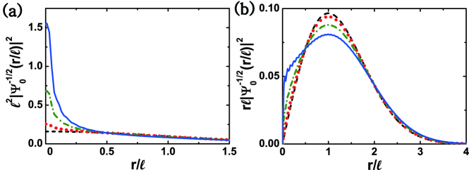
Figure 1: (a) Computed values of the probability density $\ell^{2}|\Psi_{0}^{-1/2}(r/\ell)|^{2}$ in the absence of a gap for $N_{c}=8501$. The values of $g$ are $0$ (dashed), $0.3$ (dotted), $0.5$ (dashed-dot), and $0.6$ (solid) ($\Delta=0$). Corresponding energies are $0$, $-0.382$, $-0.663$, and $-0.835$ in units of $E_{M}$. In the absence of the Coulomb potential the probability density (dashed line) at $r=0$ is $0.16$, which is much smaller than the corresponding value in the presence of the Coulomb potential. (b) Plot of the radial probability density $r\ell|\Psi_{0}^{-1/2}(r/\ell)|^{2}$. The values of $g$ are $0$ (dashed), $0.3$ (dotted), $0.5$ (dashed-dot), and $0.6$ (solid) ($\Delta=0$). The dimension of the Hamiltonian matrix is $N_{c}=8501$.

Let us first calculate probability density $\ell^{2}|\Psi_{0}^{-1/2}(r/\ell)|^{2}$ for $\Delta/E_{M}=0$. As the coupling constant increases the probability density concentrates near the center of the Coulomb potential, see Fig.1(a). It is more convenient to plot the radial probability density $(r/\ell)\ell^{2}|\Psi_{0}^{-1/2}(r/\ell)|^{2}$ instead, see Fig.1(b) and Fig.2(a): we see that for $g>1/2$ the value of the radial probability density jumps nearly discontinuously near $r=R$. This jump becomes more sharper in the limit $R\rightarrow 0$ or $1/N_{c}\rightarrow 0$. This is consistent with the scaling ansatz: the radial wavefunction diverges as $\chi_{B}(r)\sim r^{-1/2}$ near $r=0$, see Eq.(23). However, the wavefunction is normalizable. Fig.2(b) replots the radial probability density for $g=0.7$ as a function of $\frac{r}{R}\pi\sqrt{2}$. We see the curves with different values of $N_{c}$ all have the same period, approximately equal to $R$. The wavefunctions display stronger oscillations with period $R$ in comparison to those of smaller values of $g$. These are Friedel-type oscillations originating from an abrupt termination of the number of terms in the linear combination of the eigenstates, see Eq.(10).

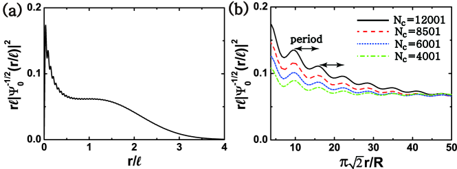
Figure 2: (a) Radial probability density $r\ell|\Psi_{0}^{-1/2}(r/\ell)|^{2}$ for $N_{c}=12001$. Here $g=0.7$ and $\Delta=0$. (b) Blow-up of the radial probability density $r\ell|\Psi_{0}^{-1/2}(r/\ell)|^{2}$ near $r\gtrsim R$ is plotted as a function of $\frac{r}{R}\pi\sqrt{2}$ for different values of $N_{c}=12001,8501,6001,4001$.

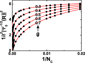
Figure 3: Inverse probability density as a function of $1/N_{c}$ for $g=0.3,0.4,0.5,0.6,0.7$. The mass gap is $\Delta=0$.

Fig.3 displays the dimensionless inverse probability density $f\Big{(}g,\frac{1}{N_{c}},0\Big{)}$ for various values of the coupling constant. Numerical result $f\Big{(}g,\frac{1}{N_{c}},0\Big{)}$ and the approximate scaling ansatz $h\Big{(}g,\frac{1}{N_{c}},0\Big{)}$ of Eq.(LABEL:main) should agree when $\frac{1}{N_{c}}\ll 1$:

$$\lim_{\frac{1}{N_{c}}\rightarrow 0}\frac{f\Big{(}g,\frac{1}{N_{c}},0\Big{)}}{h\Big{(}g,\frac{1}{N_{c}},0\Big{)}}=1.$$ (29)

This is verified by the data collapse shown in Fig.4. It confirms our scaling ansatz given in Eq.(23).

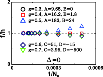
Figure 4: Data collapse of the ratio $f/h$ in the limit $1/N_{c}\rightarrow 0$ for $\Delta=0$. Here the dimension of the Hamiltonian matrix takes values $N_{c}=12001,8501,8001,7001,6001,5001,4001,3001,2401,2001$.

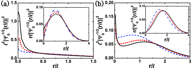
Figure 5: (a) Probability density $\ell^{2}|\Psi_{0}^{-1/2}(r/\ell)|^{2}$ as a function $r/\ell$. Values are $g=0.3$ (dashed), $0.5$ (dotted), and $0.6$ (solid). Corresponding energies are $-0.475$, $-0.741$, and $-0.897$ in units of $E_{M}$. Parameters are $J=-1/2$, $\Delta=0.1E_{M}$, and $N_{c}=8501$. Inset: radial probability density $r\ell|\Psi_{0}^{-1/2}(r/\ell)|^{2}$. (b) Probability density $\ell^{2}|\Psi_{0}^{-1/2}(r/\ell)|^{2}$ as a function $r/\ell$. Values are $g=0.3$ (dashed), $0.5$ (dotted), and $0.6$ (solid). Corresponding energies are $-1.327$, $-1.508$, and $-1.592$ in units of $E_{M}$. Parameters are $J=-1/2$, $\Delta=E_{M}$, and $N_{c}=8501$. Inset: radial probability density $r\ell|\Psi_{0}^{-1/2}(r/\ell)|^{2}$.

4.2 $\Delta\neq 0$

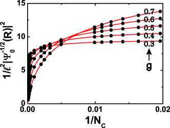
Figure 6: Inverse probability density as a function of $1/N_{c}$ for $g=0.3,0.4,0.5,0.6,0.7$. The mass gap is $\Delta=0.5E_{M}$.

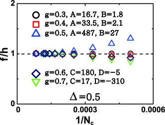
Figure 7: Data collapse of the ratio $f/h$ in the limit $1/N_{c}\rightarrow 0$ for $\Delta=0.5E_{M}$. Here the dimension of the Hamiltonian matrix takes values $N_{c}=12001,8501,8001,7001,6001,5001,4001,3001,2401,2001$.

Let us calculate probability densities for finite values of $\Delta/E_{M}$. The results for $\Delta/E_{M}=0.1$ are shown in Fig.5(a), and we see that the results are similar to those of $\Delta/E_{M}=0$. However, for a larger value $\Delta/E_{M}=1$ there is a second peak away from $r=0$, see Fig.5(b).

Fig.6 displays the dimensionless inverse probability density $f\Big{(}g,\frac{1}{N_{c}},\frac{\Delta}{E_{M}}\Big{)}$ for various values of the coupling constant. The ratio between $f\Big{(}g,\frac{1}{N_{c}},\frac{\Delta}{E_{M}}\Big{)}$ and $h\Big{(}g,\frac{1}{N_{c}},\frac{\Delta}{E_{M}}\Big{)}$ approaches $1$ in the limit $\frac{1}{N_{c}}\ll 1$, see the data collapse in Fig.7. This result suggests that, for $g\neq 0$, the value of the exponent $\nu$ is given by Eq.(23), independent of $\Delta$.

5 Results of eigenenergies

5.1 $g>1/2$

For $g>1/2$ no analytical result for eigenenergies exist. Our numerical energy values of the state $|\Psi_{0}^{-1/2}\rangle$ at $g=0.7$ and $\Delta=0$ are $E/E_{M}=-1.039,-1.063,-1.087,-1.114$ for $N_{c}=4001,6001,8501,12001$. They diverge slowly in the limit $N_{c}\rightarrow\infty$ . Similar results hold for $\Delta\neq 0$. Since $\chi_{B}(r)\sim\frac{1}{r^{1/2}}$ for small $r$ (Eq.(23)) the expectation value of the Coulomb potential is

$$E_{C}\sim\int_{R}^{\infty}drr\Big{(}r^{-\frac{1}{2}}\frac{1}{r}r^{-\frac{1}{2}}\Big{)}\sim\log(R).$$ (30)

It diverges slowly as $\log(R)$, consistent with our numerical result. Without the regularization parameter $R$ this energy diverges.

5.2 $g<1/2$

Our numerical energy values of the state $|\Psi_{0}^{-1/2}\rangle$ for $g=0.4$ converge fast as a function of $N_{c}$, in contrast to $g>1/2$. Since its radial wavefunction $\chi_{B}(r)\sim\frac{1}{r^{\nu}}$ with $\nu<1/2$ (Eq.(23)) the expectation value of the Coulomb potential is free of divergence even at $R=0$. No regularization parameter is thus needed when $g<1/2$.

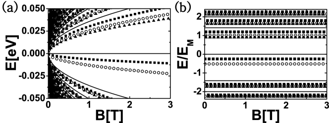
Figure 8: Eigenenergies at $g=0.4$ for angular momenta $J=-1/2$ , $J=-3/2$, and $J=1/2$, represented by circles, squares, and triangles ($\Delta=0$ and $N_{c}=8501$). Landau level energies in the absence of the Coulomb impurity ($g=0$) are represented by solid lines. In (a) eigenenergies measured in units of eV. When they are measured in units of $E_{M}$ the magnetic field dependence disappears (b).

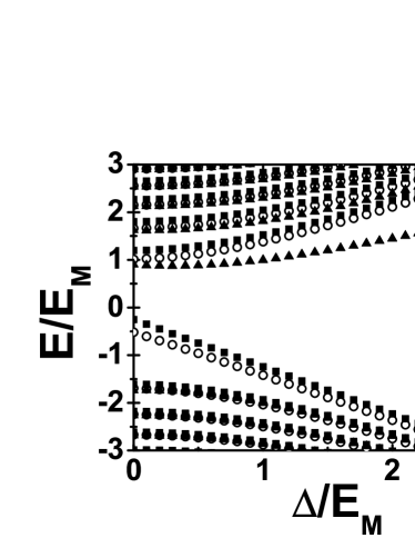
Figure 9: Eigenenergies as a function of mass gap $\Delta$ at $g=0.4$ and $N_{c}=8501$: $J=-1/2$ (circle), $J=-3/2$ (square), and $J=1/2$ (triangle).

Fig.8(a) displays eigenenergies as a function of $B$ when $\Delta=0$. The same energies in units of $E_{M}$ are displayed in Fig.8(b). The independence of $E/E_{M}$ on $B$ reflects the fact that the coupling constant $g$ is independent of $B$. Landau energy levels of graphene are also shown for comparison. The dimensionless eigenenergies for $\Delta\neq 0$ are displayed as a function of $\Delta/E_{M}$ in Fig.9. Using semiclassical analysis for small $B$ Ho and Khalilov[13] found that the first positive energy $E_{J}$ less than $\Delta$ is given by

$$\frac{E_{J}}{E_{M}}\approx\frac{\frac{\Delta}{E_{M}}+\frac{1}{2}\left(\frac{E_{M}}{\Delta}J\right)}{\left[1+\frac{g^{2}}{\left[1+\sqrt{J^{2}-g^{2}}\right]^{2}}\right]^{1/2}}$$ (31)

(See Eq.(21) in Ref.[13]). From this expression we find that $E_{J}/E_{M}\approx 9.534$ for $g=0.4$, $J=-1/2$ and $\Delta/E_{M}=10$. This value of energy agrees approximately with the numerical value $E_{J}/E_{M}\approx 9.571$. They also derived some exact solutions at denumerable number of magnetic field values (not necessarily small), and we will test our numerical results against them. According to exact results of Eq.(39) in Ref.[13] some negative energies $E_{J}$ less than $\Delta$ satisfy

$$E_{J}=-\frac{\Delta}{2(\gamma+J+1/2)},$$

$$E_{J}^{2}-\Delta^{2}=E^{2}_{M}(\gamma+1/2).$$ (32)

Solutions are

$$\frac{E_{J}}{E_{M}} = -\frac{\sqrt{\gamma+1/2}}{\sqrt{-4(\gamma+J)(\gamma+J+1)}},$$

$$\frac{\Delta}{E_{M}} = \frac{2(\gamma+J+1/2)\sqrt{\gamma+1/2}}{\sqrt{-4(\gamma+J)(\gamma+J+1)}},$$ (33)

where $\gamma=\sqrt{J^{2}-g^{2}}$, $J<0$, and $g<0.5$. For $J=-1/2$ and $g=0.4$ the solution is $(\frac{\Delta}{E_{M}},\frac{E_{J}}{E_{M}})=(0.67,-1.118)$, in agreement with the numerical result (0.67,-1.117) for $N_{c}=12001$.

6 Conclusions and discussions

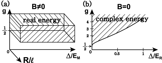
Figure 10: In the scratched regions the Coulomb potential must be regularized. (a) $B\neq 0$ and (b) $B=0$. Note that $E_{M}$ is the energy scale of graphene LLs while $E_{R}$ is the energy scale of the regularization length. We have computed electronic wavefunctions in the scratched region at $B\neq 0$.

We have explored eigenstates and eigenenergies of the Coulomb problem in a magnetic field at finite values of renormalization length $R$ and for different values of the coupling constant $g>g_{c}$. As shown in Fig.10 solutions are qualitatively different from those of zero magnetic field since the presence of a magnetic field prohibits complex energy solutions. Our numerical results show that the inverse probability density of the state $|\Psi_{0}^{-1/2}\rangle$ at $r=R$ is described by a scaling function $f(g,\frac{1}{N_{c}},\frac{\Delta}{E_{M}})$, which exhibits a significant dependence on $N_{c}$ or $R$. In the limit $N_{c}\rightarrow\infty$ the wavefunction of its s-wave component behaves as $\frac{1}{r^{\nu}}$ near $r=0$. We find that the exponent is $\nu<1/2$ when $g<1/2$ and $\nu=1/2$ when $g>1/2$, independent of mass gap[5, 14]. We thus recover the previously known results of the limit $R\rightarrow 0$, suggesting consistency of our numerical method. The wavefunctions are normalizable for all values of $g$.

In Ref.[17] an instability of many-body groundstate in magnetic fields is examined under the condition that an excited energy coincides with the Fermi energy, which is assumed to be at $E_{F}=-\Delta$ (note also the value of the Fermi energy in graphene can be tuned so it is not necessary always at $E_{F}=-\Delta$). In our single electron problem in magnetic fields this is not where the fall to the Coulomb center occurs. Instead the condition is $E\rightarrow-\infty$[1, 7].

In this paper we considered donor impurities. For acceptors or antidots[20] we can use the transformation $V(r)\rightarrow-V(r)$ with the eigenenergies $E\rightarrow-E$ (eigenstates are unchanged when $\Delta=0$). It maybe worthwhile to investigate solutions in a lattice model[21] instead of continuum models. Also the coupling between $K$ and $K^{\prime}$ valleys could provide an improved model. An experimental test of our results may be performed by measuring the transitions energies between the eigenenergies $E_{N}^{J}$.

References

- [1] J. Reinhardt, W. Greiner, Rep. Prog. Phys. 40, 219 (1977). Three dimensional Coulomb impurity problem in the absence of a magnetic field is reviewed. Analytical solutions are given.
- [2] A. K. Geim and A. H. MacDonald, Phys. Today 60, 35 (2007).
- [3] A. H. Castro Neto, F. Guinea, N. M. R. Peres, K. S. Novoselov, and A. K. Geim, Rev. Mod. Phys. 81, 109 (2009).
- [4] V. M. Pereira, J. Nilsson, and A. H. Castro Neto, Phys. Rev. Lett. 99, 166802 (2007); A. V. Shytov, M. I. Katsnelson, and L. S. Levitov, Phys. Rev. Lett. 99, 236801 (2007); V. R. Khalilov and C. L. Ho, Mod. Phys. Lett. A 13, 615 (1998).
- [5] O. V. Gamayun, E. V. Gorbar, and V. P. Gusynin, Phys. Rev. B 80, 165429 (2009).
- [6] A. H. MacDonald and D. S. Ritchie, Phys. Rev. B 33, 8336 (1986). In this paper Pade approximant is used to interpolate between low and high magnetic field limits; M.Taut, J. Phys. A: Math. Gen. 28, 2081 (1995). Analytical solutions are found at a denumerably set of magnetic fields.
- [7] L. D. Landau and E. M. Lifshitz, Quantum mechanics (3rd ed., Pergamon Press, Oxford, 1977).
- [8] The regularization parameter is the radius of the charge: or for and for .
- [9] G. Giavaras, P. A. Maksym, and M. Roy, J. Phys.: Condens. Matter 21, 102201 (2009).
- [10] A. Matulis and F. M. Peeters, Phys. Rev. B 77, 115423 (2008); P. S. Park, S. C. Kim, and S. -R. Eric Yang, Phys. Rev. Lett. 108, 169701 (2012); S. C. Kim, J. W. Lee, and S. -R. Eric Yang, J. Phys.: Condens. Matter 24, 495302 (2012).
- [11] M. V. Berry, Phys. Today 55, 10 (2002).
- [12] C. Bender and S. Orszag, Advanced Mathematical Methods for Scientists and Engineers (McGraw Hill, New York, 1978).
- [13] C. L. Ho and V. R. Khalilov, Phys. Rev. A 61, 032104 (2000).
- [14] Y. Zhang, Y. Barlas, and K. Yang, Phys. Rev. B 85, 165423 (2012).
- [15] S. -R. Eric Yang, S. Mitra, A. H. MacDonald, and M. P. A. Fisher, J. Korean Phys. Soc. 29, S10 (1996). The regularization length parameter is related to wavevector through . A wavevector can be related to the average radius through . Since state with a large LL index has radius we get .
- [16] N. Goldenfeld, Lectures on phase transitions and the renormalization group (Addison-Wesley, 1992).
- [17] O. V. Gamayun, E. V. Gorbar, and V. P. Gusynin, Phys. Rev. B 83, 235104 (2011); a different type of instability is investigated in P. S. Park, S. C. Kim, and S. -R. Eric Yang, Phys. Rev.B 84 085405 (2011).
- [18] D. Yoshioka, The Quantum Hall Effect (Springer, Berlin, 1998).
- [19] P. Recher, J. Nilsson, G. Burkard, and B. Trauzettel, Phys. Rev. B 79, 085407 (2009); M. V. Berry and R. J. Mondragon, Proc. R. Soc. Lond. A 412, 53 (1987).
- [20] P. S. Park, S. C. Kim, and S. -R. Eric Yang, J. Phys.: Condens. Matter 22 375302 (2010).
- [21] W. Zhu, Z. Wang, Q. Shi, K. Y. Szeto, J. Chen, and J. G. Hou, Phys. Rev. B 79, 155430 (2009).