Cholesky Factor Interpolation for Efficient Approximate Cross-Validation

Abstract

The dominant cost in solving least-square problems using Newton’s method is often that of factorizing the Hessian matrix over multiple values of the regularization parameter ($\lambda$). We propose an efficient way to interpolate the Cholesky factors of the Hessian matrix computed over a small set of $\lambda$ values. This approximation enables us to optimally minimize the hold-out error while incurring only a fraction of the cost compared to exact cross-validation. We provide a formal error bound for our approximation scheme and present solutions to a set of key implementation challenges that allow our approach to maximally exploit the compute power of modern architectures. We present a thorough empirical analysis over multiple datasets to show the effectiveness of our approach.

1 Introduction

Least-squares regression has continued to maintain its significance as a worthy opponent to more advanced learning algorithms. This is mainly because:

${\textbf{a}-}$ Its closed form solution can be found efficiently by maximally exploiting modern hardware using high performance BLAS-$3$ software [9].

${\textbf{b}-}$ Advances in kernel methods [28] [21] [17] can efficiently construct non-linear spaces, where the closed form solution of linear regression can be readily used.

${\textbf{c}-}$ Availability of error correcting codes [5] allow robust simultaneous learning of multiple classifiers in a single pass over the data.

However, an important bottleneck in solving large least-squares problems is the cost of $k$-fold cross validation [1]. To put this cost in perspective, we show in Figure 1 the costs of performing the main steps in solving least-squares using Newton’s method.

Specifically, for $d$-dimensional data each fold requires finding optimal value of regularization parameter $\lambda$ searched over $q$ values. This requires solving a linear system with $d$ variables, represented by the $d\times d$ Hessian matrix, $q$ times for each of the $k$ folds. As solving this system using the Cholesky factorization of the Hessian costs $\mathcal{O}(d^{3})$ operations, the total cost of $k$-folds adds up to $\mathcal{O}(kqd^{3})$ operations. Other considerable costs include computing the Hessian requiring $\mathcal{O}(nd^{2})$ operations. Comparing these costs, we see that when $n<kqd$, cross validation is the dominant cost. Figure 2 presents an empirical sense of cross-validation and Hessian costs as a function of $n$ and $d$.

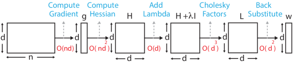
Figure 1: Computational steps for least squares regression.

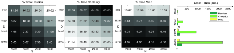
Figure 2: Percent times taken by the three main steps in least-squares pipeline for MNIST [22] data projected using polynomial kernel [17] to different sized feature spaces. In Figures a, b, and c, the x-axis represents the number of training points, while the y-axis represents the size of the feature space.

Our goal is to reduce the computational cost of cross-validation without increasing the hold-out error. To this end, we propose to densely interpolate Cholesky factors of the Hessian matrix using a sparse set of $\lambda$ values. Our key insight is that Cholesky factors for different $\lambda$ values lie on smooth curves, and can hence be approximated using polynomial functions (see Figure 3 for illustration). We provide empirical evidence supporting this intuition and provide an error bound for this approximation.

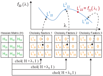
Figure 3: Given a Hessian matrix $\mathbf{H}$, we compute the Cholesky factors $\mathbf{L}^{s}$ of $\mathbf{H}+\lambda_{s}\mathbf{I}$ for a small set $\{\lambda_{s}\}$. For each $(p,q)$-th entry in these Cholesky factors ($1\leq p,q\leq d$), we fit a polynomial function $f_{p,q}(\lambda)$. These functions are used to estimate entries of $\mathbf{L}$ for a larger set of $\lambda$ values.

We formalize a least-squares framework to simultaneously learn the multiple polynomial functions required to densely interpolate the Hessian factors. An important challenge to solve this problem efficiently is a matrix-vector conversion strategy with minimal unaligned memory access (see $\S$ 5 for details). To address this challenge, we propose a general-purpose strategy to efficiently convert blocks of Choelsky factors to their corresponding vectors. This enables our learning framework to use BLAS-$3$ [9] level computations, therefore maximally exploiting the compute power of modern hardware. Our results demonstrate that the proposed approximate regularization approach offers a significant computational speed-up while providing hold-out error that is comparable to exact regularization.

2 Related Work

Solving linear systems has been well-explored in terms of their type [9] [27] and scale [18] [32]. Our focus is on the least-squares problem as the computational basis of linear regression. Popular methods to solve least-squares include QR [9], Cholesky [15], and Singular Value Decomposition (SVD) [8]. For large dense problems, Cholesky factorization has emerged as the method of choice which is used to solve the normal equation, i.e., the linear system represented by the Hessian matrix of least-squares problem. This is because of its storage ($\times 2$) and efficiency ($\times 2$ and $\times 39$) advantages over QR and SVD respectively [9]).

For real-world problems, it is common for system parameters to undergo change over time. Previous works in this context have mostly focused on low-rank updates in system parameters including direct matrix inverse [12], LU decomposition [16], Choleksy factorization [19], and Singular Value Decomposition [3] [11]. Our problem is however different in two important ways: (i) we focus on linear systems undergoing full rank updates, and (ii) our updates are limited to the diagonal of the Hessian. Both of these attributes are applicable to the regularization of least-squares problems, as we shall see in $\S$ 3.

A standard way to solve regularized least-squares is to find the SVD of the input matrix once for each training fold, and then reuse the singular vectors for different $\lambda$ values. For large problems however, finding the SVD of a design matrix even once can be prohibitively expensive. In such situations, truncated [14] or randomized approximate [13] SVD can be used. However their effectiveness for optimizing hold-out error for least squares problems is still unexplored. There has also been work to reduce the number of regularization folds [4] by minimizing the regularizing path [6]. Our work can be used in conjunction with these approaches to further improve the overall performance.

3 piCholesky Framework

3.1 Preliminaries

Let $\mathbf{X}$ be the $n\times(d+1)$ design matrix with each row as one of the $n$ training examples in a $d$-dimensional space. Let $\mathbf{y}$ be the $n$ dimensional vector for training labels. Then the Tychonov regularized [31] least-squares cost function $\mathbf{J(\theta)}$ is given as:

$$\mathbf{J(\theta)}=\frac{1}{2}(\mathbf{y}-\mathbf{X\theta})^{\top}(\mathbf{y}-\mathbf{X\theta})+\frac{\lambda}{2}\mathbf{\theta}^{\top}\mathbf{\theta}$$ (1)

Setting the derivative of $\mathbf{J(\theta)}$ with respect to $\mathbf{\theta}$ equal to zero results in the following solution of $\theta$:

$$\mathbf{\theta}=(\mathbf{H}+\lambda\mathbf{I})^{-1}\mathbf{g}$$ (2)

where $\mathbf{I}$ is the $(d+1)\times(d+1)$ identity matrix, the Hessian matrix $\mathbf{H}$ equals $\mathbf{X}^{\top}\mathbf{X}$ and the gradient vector $\mathbf{g}$ is $\mathbf{X}^{\top}\mathbf{y}$. Equation 2 is solved for different values of $\lambda$ in a k-fold cross-validation setting, and the $\lambda$ with minimum hold-out error in expectation is picked.

3.2 Least Squares using Cholesky Factors

Rewriting Equation 2 as $\mathbf{A}\theta=\mathbf{g}$, where $\mathbf{A}$ $=$ $\mathbf{H}+\lambda\mathbf{I}$, we can find Cholesky factors of $\mathbf{A}$ as $\mathbf{A}=\mathbf{L}\mathbf{L}^{\textrm{T}}$, where $\mathbf{L}$ is a lower-triangular matrix. Equation 2 can now be written as $\mathbf{L}\mathbf{L}^{\textrm{T}}\theta=\mathbf{g}$. Using $\mathbf{L}^{\textrm{T}}\theta$ as $\mathbf{w}$, this can be solved by a forward-substitution to solve the triangular system $\mathbf{L}\mathbf{w}=\mathbf{g}$ for $\mathbf{w}$ followed by a back-substitution to solve the triangular system $\mathbf{L}^{\textrm{T}}\theta=\mathbf{w}$ for $\theta$.

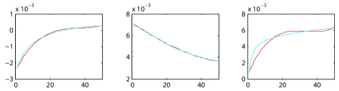
Figure 4: Plots for subset of entries in $\mathbf{L}$ (y-axes) for different $\lambda$ values (x-axes) on MNIST data. The red curves use exact Cholesky over $50$ $\lambda$ values, while the blue curves show the interpolated values of $\mathbf{L}$ evaluated from $2^{\textrm{nd}}$ order polynomials learned using $6$ values of $\lambda$.

3.3 Cholesky Factors Interpolation

To minimize the computational cost for cross-validation, we propose to compute Cholesky factors $\mathbf{L}\mathbf{L}^{\textrm{T}}$ of $\mathbf{A}$ over a small set of $\lambda$ values, followed by interpolating the corresponding entries in $\mathbf{L}$ for a more densely sampled set of $\lambda$ values. Note that corresponding entries of $\mathbf{L}$ for different values of $\lambda$ lie on smooth curves that can be accurately approximated using multiple polynomial functions. Figure 4 illustrates this point empirically, where the red curves show multiple corresponding entries in $\mathbf{L}$ computed over different $\lambda$ values using exact Cholesky for MNIST data.

Recall that for $d$-dimensional data, there are $\textrm{D}=(d+1)(d+2)/2$ number of entries in the lower-triangular part of $\mathbf{L}$. Therefore, to interpolate a Cholesky factor based on those computed for different values of $\lambda$, we need to learn D polynomial functions, each for an entry in the lower-triangular part of $\mathbf{L}$.

This challenge can be posed as a least-squares problem. Recall that each polynomial function to be learned is of order $r$. We therefore need $g>r$ exact Cholesky factors, each of which is computed using one of the $g$ values of $\lambda$. We evaluate a polynomial basis of the space of $r$-th order polynomials at the sparsely sampled $g$ values of $\lambda$ (e.g., $1,\lambda$, and $\lambda^{2}$ for second-order polynomials); this way, we form our $g\times(r+1)$ observation matrix $\mathbf{V}$. Our targets are the $g$ rows of D values, where each row corresponds to the exact Cholesky matrix computed for one of the $g$ values of $\lambda$. This forms our $g\times\textrm{D}$ target matrix $\mathbf{T}$.

In Algorithm 1, we use monomials as the polynomial basis to interpolate the $r$th-order polynomials. While we can employ other polynomial bases that are numerically more stable (such as Chebyshev polynomials), we found in our experiments that the observation matrix $\mathbf{V}$ is well-conditioned and therefore using monomials does not harm our numerical stability.

Algorithm 1 – piCholesky

Input: Degree $r$, $\{\lambda_{s}\}$ for $s=\{1,2,\cdot\cdot g\}$, $g>r$
Output: A $(r+1)\times\textrm{D}$ coefficient matrix $\Theta$, where $\textrm{D}=(d+1)(d+2)/2$ and $d$ is the data dimensionality

1:Find $\mathbf{L}^{s}=\textrm{chol}(\mathbf{H}+\lambda_{s}\mathbf{I})$ for $s=\{1,2,\cdot\cdot\cdot g\}$

2:Convert each $\mathbf{L}^{s}$ into a row vector to construct the $g\times\textrm{D}$ target matrix $\mathbf{T}$

3:Find the $g\times g$ Vandermonde matrix $\mathbf{W}$

4:Extract the leftmost $(r+1)$ colums of $\mathbf{W}$ to form the $g\times(r+1)$ observation matrix $\mathbf{V}$

5:Find $\mathbf{G}_{\lambda}=\mathbf{V}^{\textrm{T}}\mathbf{T}$ and $\mathbf{H}_{\lambda}=\mathbf{V}^{\textrm{T}}\mathbf{V}$

6:Find $\Theta=\mathbf{H}_{\lambda}^{-1}\mathbf{G}_{\lambda}$

We can now define our cost function $\mathbf{J}_{\lambda}(\Theta)$ as:

$$\mathbf{J}_{\lambda}(\Theta)=\frac{1}{2}(\mathbf{T}-\mathbf{V}\Theta)^{\top}(\mathbf{T}-\mathbf{V}\Theta)$$ (3)

where $\Theta$ is the $(r+1)\times\textrm{D}$ polynomial coefficient matrix. Each column of $\Theta$ represents the $(r+1)$ coefficients of the D polynomial functions. Following procedure similar to $\S$ 3.1, the expression of $\Theta$ can be written as

$$\Theta=\mathbf{H}_{\lambda}^{-1}\mathbf{G}_{\lambda}$$ (4)

Here $\mathbf{H}_{\lambda}=\mathbf{V}^{\textrm{T}}\mathbf{V}$, and $\mathbf{G}_{\lambda}=\mathbf{V}^{\textrm{T}}\mathbf{T}$.

Given a new regularization parameter value $\lambda_{t}$, the value for $\mathbf{L}^{t}$ can be computed by evaluating the D polynomial functions at $\lambda_{t}$. This procedure is listed in Algorithm 1. The interpolation results using Algorithm 1 for the Cholesky factors computed on the MNIST data [22] are shown with blue curves in Figure 4. Here we set $g=5$ and $r=2$. As can be seen from the figure, the blue plots (interpolated) trace the red plots (exact) closely.

Computational Complexity: The dominant step of Algorithm 1 is evaluating $\mathbf{L}^{s}$ for $s=1,2,\cdots,g$, which requires $\mathcal{O}(gd^{3})$ operations. The only other noteworthy steps of Algorithm 1 are finding $\mathbf{G}_{\lambda}$ and $\Theta$ each of which takes $\mathcal{O}(grd^{2})$ operations. Since $d>>r$, the overall asymptotic cost of Algorithm 1 is $\mathcal{O}(gd^{3})$. Furthermore, it only takes $\mathcal{O}(rd^{2})$ operations to evaluate the interpolated Cholesky factor $\mathbf{L}^{t}$ for each $\lambda_{t}$ value.

4 Theoretical Analysis

There are two challenges in developing a reasonable bound on the error of the piCholesky algorithm. The first is determining the extent to which the Cholesky factorization can be approximated entrywise as a polynomial: if one explicitly forms the symbolic Cholesky factorization of even a $3\times 3$ matrix, it is not clear at all that the entries of the resulting Cholesky factor can be approximated well by any polynomial. The second is determining the extent to which the particular polynomial recovered by the piCholesky procedure of solving a least squares system (Algorithm 1) is a good polynomial approximation to the Cholesky factorization.

The classical tool for addressing the first challenge is the Bramble-Hilbert lemma [2][Lemma 4.3.8], which guarantees the existence of a polynomial approximation to a smooth function on a compact domain, with Sobolev norm approximation error bounded by the Sobolev norm of the derivatives of the function itself. Our proof of the existence of a polynomial approximation to the Cholesky factorization is very much in the spirit of the Bramble-Hilbert lemma, but provides sharper results than the direct application of the lemma itself (essentially because we do not care about the error in approximating the derivatives of the Cholesky factorization). We surmount the second obstacle by noting that, if instead of sampling the Cholesky factorization itself when following the piCholesky procedure, we sample from a polynomial approximation to the Cholesky factorization, then the error in the resulting polynomials can be bounded using results on the stability of the solution to perturbed linear systems.

In our arguments, we find it convenient to use the Fréchet derivative: given a mapping $f:X\rightarrow Y$ between two normed linear linear spaces we define $Df$, the derivative of $f$, to be the function that maps $\mathbf{u}\in X$ to $D_{\mathbf{u}}f:X\rightarrow Y$, the unique linear map (assuming it exists) that is tangent to $f$ at $\mathbf{u}$ in the sense that

$$\lim_{\|\boldsymbol{\delta}\|_{X}\rightarrow 0}\frac{\|f(\mathbf{u}+\boldsymbol{\delta})-f(\mathbf{u})-D_{\mathbf{u}}f(\boldsymbol{\delta})\|_{Y}}{\|\boldsymbol{\delta}\|_{X}}=0,$$

The Fréchet derivative generalizes the conventional derivative, so it follows a chain rule, can be used to form Taylor Series expansions, and shares the other properties of the conventional derivative [24].

We inductively define the $r$th derivative of $f,$ $D^{r}f$, as the function that maps $\mathbf{u}\in X$ to the unique linear map tangent to $D^{r-1}_{\mathbf{u}}f$ at $\mathbf{u}$ in the sense that

$$\lim_{\|\boldsymbol{\delta}_{1}\|_{X}\rightarrow 0}\frac{\|D^{r-1}_{\mathbf{u}+\boldsymbol{\delta}_{1}}f(\boldsymbol{\delta}_{2})-D^{r-1}_{\mathbf{u}}f(\boldsymbol{\delta}_{2})-D^{r}_{\mathbf{u}}f(\boldsymbol{\delta}_{1},\boldsymbol{\delta}_{2})\|_{Y}}{\|\boldsymbol{\delta}_{1}\|_{X}}=0.$$

For a comprehensive introduction to Fréchet derivatives and their properties, we refer the reader to [24].

4.1 Performance Guarantee for piCholesky

Let $\mathbf{p}_{\mathrm{TS}}(\lambda;\lambda_{\textrm{c}})$ denote the second-order polynomial obtained from the Taylor Series expansion of $\mathcal{C}(\mathbf{A}+\lambda\mathbf{I})$ around $\lambda=\lambda_{\textrm{c}}$ and let $\mathbf{p}_{\pi}(\lambda)$ denote the approximation to $\mathcal{C}(\mathbf{A}+\lambda\mathbf{I})$ obtained using the piCholesky procedure. Our argument consists in bounding the errors in approximating $\mathcal{C}$ with $\mathbf{p}_{\mathrm{TS}}$ (Theorem 4.4) and in approximating $\mathbf{p}_{\mathrm{TS}}$ with $\mathbf{p}_{\pi}$ (Theorem 4.6). The root mean-squared error in approximating $\mathcal{C}(\mathbf{A}+\lambda\mathbf{I})$ with the piCholesky procedure is then controlled using the triangle inequality (Theorem 4.7): if $\gamma=|\lambda-\lambda_{\textrm{c}}|$ and $w=\max_{i}|\lambda_{i}-\lambda_{\textrm{c}}|$ is the maximum distance of any of the sample points used in Algorithm 1 from $\lambda_{\textrm{c}}$, then

$$\frac{1}{\sqrt{D}}\|\mathcal{C}(\mathbf{A}+\lambda\mathbf{I})-\mathbf{p}_{\pi}(\lambda)\|_{F}\leq\big{[}\gamma^{3}+\sqrt{g}w^{3}(1+\gamma^{2})(\lambda_{\textrm{c}}+1)\|\mathbf{V}^{\dagger}\|_{2}\big{]}\frac{\mathrm{R}_{[\lambda_{\textrm{c}}-\gamma,\lambda_{\textrm{c}}+\gamma]}}{\sqrt{D}}$$ (5)

Here, $g$ is the number of sample points (values of $\lambda$) used in the piCholesky procedure, $D=(d+1)(d+2)/2$ is the number of elements in $\mathcal{C}(\mathbf{A}+\lambda\mathbf{I})$, and $\mathrm{R}_{[a,b]}$ is defined in Theorem 4.4. The quantity $\mathrm{R}_{[a,b]}$ measures the magnitude of the third-derivative of $\mathcal{C}(\mathbf{A}+\lambda\mathbf{I})$ over the interval $\lambda\in[a,b]$; when it is small, the implicit assumption made by the piCholesky procedure that $\mathcal{C}$ is well-approximated by some quadratic polynomial is reasonable. Unfortunately the task of relating $\mathrm{R}_{[a,b]}$ to more standard quantities such as the eigenvalues of $\mathbf{A}$ is beyond the reach of our analysis.

The matrix $\mathbf{V}$ (defined in Algorithm 1) is a submatrix of the Vandermonde matrix formed by the sample points, so the quantity $\|\mathbf{V}^{\dagger}\|_{2}$ measures the conditioning of the sample points used to fit the piCholesky polynomial approximant: it is small when the $g$ rows of $\mathbf{V}$ are linearly independent. This is exactly the setting in which we expect the least-squares fit in Algorithm 1 to be most stable.

The cubic dependence on $\gamma=|\lambda-\lambda_{\textrm{c}}|$ in our bound reflects our intuition that since the Cholesky factorization is nonlinear, we do not expect the quadratic approximation formed using the piCholesky procedure to perform well far away from the interpolation points used to form the approximation. The cubic dependence on $w=\max_{i}|\lambda_{i}-\lambda_{\textrm{c}}|$ also captures our intuition that we can only expect piCholesky to give a good approximation when the interpolation points used to fit the interpolant cover a small interval containing the optimal regularization parameter.

To algorithmically address the fact that this optimal $\lambda_{\textrm{c}}$ is unknown, we introduce a Multi-level Cholesky procedure in Section 6.2 that applies a binary-search-like procedure to narrow the search range before applying piCholesky.

4.2 Proof of the performance guarantee for piCholesky

Our first step in developing the Taylor series of $\mathcal{C}(\mathbf{A})$ is establishing that $\mathcal{C}$ is indeed Fréchet differentiable, and finding an expression for the derivative.

Theorem 4.1.

Assume $\mathbf{A}$ is a positive-definite matrix and $\mathcal{C}(\mathbf{A})=\mathbf{L}.$ Then $D_{\mathbf{L}}\mathcal{S}(\boldsymbol{\Gamma})=\boldsymbol{\Gamma}\mathbf{L}^{T}+\mathbf{L}\boldsymbol{\Gamma}^{T}$ for any lower-triangular matrix $\boldsymbol{\Gamma}$ and $D_{\mathbf{L}}\mathcal{S}$ is full-rank. Furthermore, if $\mathbf{\Delta}$ is a symmetric matrix, then

$$D_{\mathbf{A}}\mathcal{C}(\boldsymbol{\Delta})=\left(D_{\mathbf{L}}\mathcal{S}\right)^{-1}(\boldsymbol{\Delta}).$$

To key to establishing this result is the observation that $\mathcal{C}$ is the inverse of the mapping $\mathcal{S}:\mathbf{L}\mapsto\mathbf{LL}^{T}$ that maps the set of lower-triangular matrices into the set of symmetric matrices. Differentiability of $\mathcal{C}$ is then a consequence of the following corollary of the Inverse Function Theorem (Theorem 2.5.2 of [24]).

Theorem 4.2.

Let $f:X\rightarrow Y$ be continuously differentiable. If $Df(\mathbf{u})$ is invertible, then

$$D(f^{-1})_{f(\mathbf{u})}=\left(Df_{\mathbf{u}}\right)^{-1}.$$

Proof of Theorem 4.1.

By Theorem 4.2 and the fact that $\mathcal{C}=\mathcal{S}^{-1},$ it suffices to establish that $\mathcal{S}$ is continuously differentiable with $D\mathcal{S}_{\mathbf{L}}(\boldsymbol{\Gamma})=\boldsymbol{\Gamma}\mathbf{L}^{T}+\mathbf{L}\boldsymbol{\Gamma}^{T}$ and that $D\mathcal{S}_{\mathbf{L}}$ is invertible.

Recall that (assuming it exists), $D\mathcal{S}_{\mathbf{L}}$ is the unique linear map tangent to $\mathcal{S}$ at $\mathbf{L}$ and observe that

$$\mathcal{S}(\mathbf{L}+\boldsymbol{\Gamma}) =\mathbf{LL}^{T}+\boldsymbol{\Gamma}\mathbf{L}^{T}+\mathbf{L}\boldsymbol{\Gamma}+\boldsymbol{\Gamma}\boldsymbol{\Gamma}^{T}$$

$$=\mathcal{S}(\mathbf{L})+\boldsymbol{\Gamma}\mathbf{L}^{T}+\mathbf{L}\boldsymbol{\Gamma}+\mathrm{O}(\|\boldsymbol{\Gamma}\|^{2}).$$

It follows that $D\mathcal{S}_{\mathbf{L}}$ exists and is as stated. Clearly $D\mathcal{S}_{\mathbf{L}}$ is also continuous as a function of $\mathbf{L},$ so $\mathcal{S}$ is continuously differentiable.

To show that $D\mathcal{S}_{\mathbf{L}}$ is invertible, assume that $\boldsymbol{\Gamma}$ is such that $D\mathcal{S}_{\mathbf{L}}(\boldsymbol{\Gamma})=\boldsymbol{\Gamma}\mathbf{L}^{T}+\mathbf{L}\boldsymbol{\Gamma}^{T}=\mathbf{0}.$ Because $\mathbf{A}$ is positive-definite, $\mathbf{L}$ is invertible, and we can conclude that $\mathbf{L}^{-1}\boldsymbol{\Gamma}=-\boldsymbol{\Gamma}^{T}(\mathbf{L}^{-1})^{T}.$ The left hand side is a lower triangular matrix since $\mathbf{L}^{-1}$ and $\boldsymbol{\Gamma}$ are lower-triangular; for similar reasons, the the right hand side is upper-triangular. It follows that $\mathbf{L}^{-1}\boldsymbol{\Gamma}$ is a diagonal matrix, and hence $\boldsymbol{\Gamma}=\mathbf{L}\mathbf{D}$ for some diagonal matrix $\mathbf{D}.$ Together with the assumption that $\boldsymbol{\Gamma}\mathbf{L}^{T}+\mathbf{L}\boldsymbol{\Gamma}^{T}=\mathbf{0},$ this implies that $2\mathbf{LDL}^{T}=\boldsymbol{\Gamma}\mathbf{L}^{T}+\mathbf{L}\boldsymbol{\Gamma}^{T}=\mathbf{0}$, and consequently $\mathbf{D}=\mathbf{0}.$ Thus $\boldsymbol{\Gamma}=\mathbf{0},$ so we have established that the nullspace of $D\mathcal{S}_{\mathbf{L}}$ is $\mathbf{0}.$ It follows that $D\mathcal{S}_{\mathbf{L}}$ is invertible.

The claims of Theorem 4.1 now follow. ∎

The higher-order derivatives of $\mathcal{C}$ are cumbersome, so instead of dealing directly with $\mathcal{C}$, which maps matrices to matrices, we compute the higher-order derivatives of the equivalent function $C=\mathrm{vec}\circ\mathcal{C}\circ\mathrm{vec}^{-1}$ that maps vectors to vectors. The following theorem gives the first three derivatives of $C.$

Theorem 4.3.

Let $X,Y\subset\mathbb{R}^{d^{2}}$ be the image under $\mathrm{vec}\left(\cdot\right)$ of, respectively, the set of positive-definite matrices of order $d$ and the space of lower-triangular matrices of order $d.$ Define $C:X\rightarrow Y$ by

$$C=\mathrm{vec}\circ\mathcal{C}\circ\mathrm{vec}^{-1}.$$

When $\mathbf{A}$ is positive-definite, the first three derivatives of $C$ at $\mathbf{v_{A}}$ are given by

$$D_{\mathbf{v_{A}}}C(\boldsymbol{\delta}_{1}) =\mathbf{M}^{-1}\boldsymbol{\delta}_{1},$$

$$D_{\mathbf{v_{A}}}^{2}C(\boldsymbol{\delta}_{1},\boldsymbol{\delta}_{2}) =-\mathbf{M}^{-1}\cdot\llbracket\mathrm{vec}^{-1}(\mathbf{M}^{-1}\boldsymbol{\delta}_{1})\rrbracket\cdot\mathbf{M}^{-1}\boldsymbol{\delta}_{2},$$

$$D_{\mathbf{v_{A}}}^{3}C(\boldsymbol{\delta}_{1},\boldsymbol{\delta}_{2},\boldsymbol{\delta}_{3}) =\mathbf{M}^{-1}\cdot\Big{(}\llbracket\mathrm{vec}^{-1}(\mathbf{M}^{-1}\boldsymbol{\delta}_{1})\rrbracket\cdot\mathbf{M}^{-1}\cdot\llbracket\mathrm{vec}^{-1}(\mathbf{M}^{-1}\boldsymbol{\delta}_{2})\rrbracket$$

$$\quad\quad\quad\quad+\llbracket\mathrm{vec}^{-1}(\mathbf{M}^{-1}\cdot\llbracket\mathrm{vec}^{-1}(\mathbf{M}^{-1}\boldsymbol{\delta}_{1})\rrbracket\cdot\mathbf{M}^{-1}\boldsymbol{\delta}_{2})\rrbracket$$

$$\quad\quad\quad\quad+\llbracket\mathrm{vec}^{-1}(\mathbf{M}^{-1}\boldsymbol{\delta}_{2})\rrbracket\cdot\mathbf{M}^{-1}\cdot\llbracket\mathrm{vec}^{-1}(\mathbf{M}^{-1}\boldsymbol{\delta}_{1}))\rrbracket\Big{)}\cdot\mathbf{M}^{-1}\boldsymbol{\delta}_{3},$$

where $\mathbf{M}=\llbracket\mathcal{C}(\mathbf{A})\rrbracket.$

Proof.

First we convert the expression for $D_{\mathbf{A}}\mathcal{C}$ given in Theorem 4.1 into an expression for $D_{\mathbf{v_{A}}}C.$ To do so, we note that $\mathrm{vec}\left(\cdot\right)$ and $\mathrm{vec}\left(\cdot\right)^{-1}$ are linear functions, so are their own derivatives. It follows from the Chain Rule (Theorem 2.4.3 of [24]) that

$$DC=\mathrm{vec}\circ D\mathcal{C}\circ\mathrm{vec}^{-1},$$

so

$$D_{\mathbf{v_{A}}}C(\mathbf{v}_{\boldsymbol{\Delta}})=\mathrm{vec}\left(D_{\mathbf{A}}\mathcal{C}(\boldsymbol{\Delta})\right).$$

By Theorem 4.1, $D_{\mathbf{A}}\mathcal{C}(\boldsymbol{\Delta})=\boldsymbol{\Gamma},$ where $\boldsymbol{\Gamma}$ is the solution to the equation

$$\boldsymbol{\Delta}=\boldsymbol{\Gamma}\mathcal{C}(\mathbf{A})^{T}+\mathcal{C}(\mathbf{A})\boldsymbol{\Gamma}^{T}.$$

We can convert this to an equation for $\mathbf{v}_{\boldsymbol{\Gamma}}$ using the fact (Section 10.2.2 of [26]) that

$$\mathrm{vec}\left(\mathbf{ABC}\right)=(\mathbf{C}^{T}\otimes\mathbf{A})\mathrm{vec}\left(\mathbf{B}\right)$$

for arbitrary matrices $\mathbf{A},\mathbf{B},$ and $\mathbf{C}.$ Specifically, we find that $\mathbf{v}_{\boldsymbol{\Gamma}}$ satisfies

$$\mathbf{v}_{\boldsymbol{\Delta}}=(\mathcal{C}(\mathbf{A})\otimes\mathbf{I})\mathbf{v}_{\boldsymbol{\Gamma}}+(\mathbf{I}\otimes\mathcal{C}(\mathbf{A}))\mathbf{v}_{\boldsymbol{\Gamma}^{T}}.$$

Recall that $\boldsymbol{\Delta}$ is symmetric, so $\mathbf{v}_{\boldsymbol{\Gamma}^{T}}=\mathbf{v}_{\boldsymbol{\Gamma}}$ and we have that

$$\mathbf{v}_{\boldsymbol{\Gamma}}=\llbracket\mathcal{C}(\mathbf{A})\rrbracket^{-1}\mathbf{v}_{\boldsymbol{\Delta}}.$$

It follows that

$$D_{\mathbf{v_{A}}}C(\mathbf{v}_{\boldsymbol{\Delta}})=\mathrm{vec}\left(D_{\mathbf{A}}\mathcal{C}(\boldsymbol{\Delta})\right)=\mathrm{vec}\left(\boldsymbol{\Gamma}\right)=v_{\boldsymbol{\Gamma}}=\llbracket\mathcal{C}(\mathbf{A})\rrbracket^{-1}\mathbf{v}_{\boldsymbol{\Delta}}=\mathbf{M}^{-1}\mathbf{v}_{\boldsymbol{\Delta}}$$

as claimed.

To compute the second derivative of $C,$ we use the identity (Section 2.2 of [26])

$$D_{\mathbf{x}}A(\mathbf{x})^{-1}=-A(\mathbf{x})^{-1}\cdot D_{\mathbf{x}}A(\mathbf{x})\cdot A(\mathbf{x})^{-1}$$ (6)

that holds for any differentiable matrix-valued function of $\mathbf{x}.$ Using this identity with $\mathbf{x}=\mathbf{v_{\mathbf{A}}}$ and $A=\mathbf{M},$ we see that

$$D^{2}_{\mathbf{v_{A}}}C(\boldsymbol{\delta}_{1},\boldsymbol{\delta}_{2})=D_{\mathbf{v_{A}}}(D_{\mathbf{v_{A}}}C(\boldsymbol{\delta}_{2}))(\boldsymbol{\delta}_{1}) =D_{\mathbf{v_{A}}}(\mathbf{M}^{-1}\boldsymbol{\delta}_{2})(\boldsymbol{\delta}_{1})=D_{\mathbf{v_{A}}}(\mathbf{M}^{-1})(\boldsymbol{\delta}_{1})\cdot\boldsymbol{\delta}_{2}$$

$$=-\mathbf{M}^{-1}\cdot D_{\mathbf{v_{A}}}\mathbf{M}(\boldsymbol{\delta}_{1})\cdot\mathbf{M}^{-1}\cdot\boldsymbol{\delta}_{2}.$$

Using the Chain Rule and the linearity of $\llbracket\mathrm{vec}^{-1}(\cdot)\rrbracket,$ we see that

$$D_{\mathbf{v_{A}}}\mathbf{M}(\boldsymbol{\delta}_{1}) =D_{\mathbf{v_{A}}}\llbracket\mathcal{C}(\mathbf{A})\rrbracket(\boldsymbol{\delta}_{1})=D_{\mathbf{v_{A}}}\llbracket\mathrm{vec}^{-1}(C(\mathbf{v_{A}}))\rrbracket(\boldsymbol{\delta}_{1})$$

$$=\left\llbracket\mathrm{vec}^{-1}\left(D_{\mathbf{v_{A}}}C(\mathbf{v_{A}})(\boldsymbol{\delta}_{1})\right)\right\rrbracket=\llbracket\mathrm{vec}^{-1}(\mathbf{M}^{-1}\boldsymbol{\delta}_{1})\rrbracket.$$ (7)

Thus, as claimed,

$$D_{\mathbf{v_{A}}}^{2}C(\boldsymbol{\delta}_{1},\boldsymbol{\delta}_{2})=-\mathbf{M}^{-1}\cdot\llbracket\mathrm{vec}^{-1}(\mathbf{M}^{-1}\boldsymbol{\delta}_{1})\rrbracket\cdot\mathbf{M}^{-1}\boldsymbol{\delta}_{2}.$$

To compute the third derivative of $C,$ we note that the Product Rule (Theorem 2.4.4 of [24]) implies

$$D_{\mathbf{x}}[A_{1}(\mathbf{x})\cdot A_{2}(\mathbf{x})\cdot A_{1}(\mathbf{x})]=D_{\mathbf{x}}A_{1}(\mathbf{x})\cdot A_{2}(\mathbf{x})\cdot A_{1}(\mathbf{x})+A_{1}(\mathbf{x})\cdot D_{\mathbf{x}}A_{2}(\mathbf{x})\cdot A_{1}(\mathbf{x})+A_{1}(\mathbf{x})\cdot A_{2}(\mathbf{x})\cdot D_{\mathbf{x}}A_{1}(\mathbf{x})$$

for any matrix-valued differentiable functions $M_{1}$ and $M_{2}.$ We apply this result with $\mathbf{x}=\mathbf{v_{A}},$ $A_{1}=\mathbf{M}^{-1},$ and $A_{2}=\llbracket\mathrm{vec}^{-1}(\mathbf{M}^{-1}\boldsymbol{\delta}_{2})\rrbracket$ to see that

$$D_{\mathbf{v_{A}}}^{3}C(\boldsymbol{\delta}_{1},\boldsymbol{\delta}_{2},\boldsymbol{\delta}_{3})=D_{\mathbf{v_{A}}}(D_{\mathbf{v_{A}}}^{2}C(\boldsymbol{\delta}_{2},\boldsymbol{\delta}_{3}))(\boldsymbol{\delta}_{1}) =-D_{\mathbf{v_{A}}}\mathbf{M}^{-1}(\boldsymbol{\delta}_{1})\cdot\llbracket\mathrm{vec}^{-1}(\mathbf{M}^{-1}\boldsymbol{\delta}_{2})\rrbracket\cdot\mathbf{M}^{-1}\boldsymbol{\delta}_{3}$$

$$-\mathbf{M}^{-1}\cdot D_{\mathbf{v_{A}}}\llbracket\mathrm{vec}^{-1}(\mathbf{M}^{-1}\boldsymbol{\delta}_{2})\rrbracket(\boldsymbol{\delta}_{1})\cdot\mathbf{M}^{-1}\boldsymbol{\delta}_{3}$$

$$-\mathbf{M}^{-1}\cdot\llbracket\mathrm{vec}^{-1}(\mathbf{M}^{-1}\boldsymbol{\delta}_{2})\rrbracket\cdot D_{\mathbf{v_{A}}}\mathbf{M}^{-1}(\boldsymbol{\delta}_{1})\cdot\boldsymbol{\delta}_{3}.$$ (8)

From (6) and (7), we calculate

$$D_{\mathbf{v_{A}}}\mathbf{M}^{-1}(\boldsymbol{\delta}_{1})=-\mathbf{M}^{-1}\cdot D_{\mathbf{v_{A}}}\mathbf{M}(\boldsymbol{\delta}_{1})\cdot\mathbf{M}^{-1}=-\mathbf{M}^{-1}\cdot\llbracket\mathrm{vec}^{-1}(\mathbf{M}^{-1}\boldsymbol{\delta}_{1})\rrbracket\cdot\mathbf{M}^{-1},$$

and to calculate $D_{\mathbf{v_{A}}}\llbracket\mathrm{vec}^{-1}(\mathbf{M}^{-1}\boldsymbol{\delta}_{2})\rrbracket(\boldsymbol{\delta}_{1}),$ we use the fact that $\llbracket\mathrm{vec}^{-1}(\cdot)\rrbracket$ is linear:

$$D_{\mathbf{v_{A}}}\llbracket\mathrm{vec}^{-1}(\mathbf{M}^{-1}\boldsymbol{\delta}_{2})\rrbracket(\boldsymbol{\delta}_{1}) =\llbracket\mathrm{vec}^{-1}((D_{\mathbf{v_{A}}}\mathbf{M}^{-1})(\boldsymbol{\delta}_{1})\cdot\boldsymbol{\delta}_{2})\rrbracket$$

$$=\llbracket\mathrm{vec}^{-1}(-\mathbf{M}^{-1}\cdot\llbracket\mathrm{vec}^{-1}(\mathbf{M}^{-1}\boldsymbol{\delta}_{1})\rrbracket\cdot\mathbf{M}^{-1}\cdot\boldsymbol{\delta}_{2})\rrbracket.$$

The claimed expression for $D_{\mathbf{v_{A}}}^{3}C$ follows from using these latter two computations to expand (8). ∎

Now that we have the first three derivatives of $\mathcal{C},$ we can develop the second-order Taylor Series expansion of $\mathcal{C}(\mathbf{A})$ and bound the error of the approximation.

Theorem 4.4.

Assume $\mathbf{A}$ is an positive-definite matrix of order $d+1$ and let $\mathbf{v_{I}}=\mathrm{vec}\left(\mathbf{I}\right),$ $\mathbf{M}_{s}=\llbracket\mathcal{C}(\mathbf{A}+s\mathbf{I})\rrbracket,$ and $\mathbf{E}_{s}=\llbracket\mathrm{vec}^{-1}(\mathbf{M}_{s}^{-1}\mathbf{v_{I}})\rrbracket.$ The second-order Taylor Series approximation to $\mathcal{C}(\mathbf{A}+\lambda\mathbf{I})$ at $\lambda=\lambda_{\textrm{c}}$ is

$$\mathbf{p}_{\mathrm{TS}}(\lambda;\lambda_{\textrm{c}})=\mathcal{C}(\mathbf{A}+\lambda_{\textrm{c}}\mathbf{I})+\mathrm{vec}^{-1}\left((\lambda-\lambda_{\textrm{c}})\mathbf{M}_{\textrm{c}}^{-1}\mathbf{v_{I}}-\frac{(\lambda-\lambda_{\textrm{c}})^{2}}{2}\mathbf{M}_{\textrm{c}}^{-1}\mathbf{E}_{\textrm{c}}\mathbf{M}_{\textrm{c}}^{-1}\mathbf{v_{I}}\right).$$

Let $D=(d+1)(d+2)/2;$ then for any $\lambda,\lambda_{\textrm{c}}>0,$

$$\frac{1}{\sqrt{D}}\|\mathcal{C}(\mathbf{A}+\lambda\mathbf{I})-\mathbf{p}_{\mathrm{TS}}(\lambda;\lambda_{\textrm{c}})\|_{F}\leq\frac{2|\lambda-\lambda_{\textrm{c}}|^{3}}{3\sqrt{D}}\mathrm{R}_{[\lambda_{\textrm{c}},\lambda]}$$

where

$$\mathrm{R}_{[a,b]}:=\max_{s\in[\mathrm{min}(a,b),\mathrm{max}(a,b)]}\left(\|\mathbf{M}_{s}^{-1}\mathbf{E}_{s}\|_{2}^{2}\|\mathbf{M}_{s}^{-1}\mathbf{v_{I}}\|_{2}+\|\mathbf{M}_{s}^{-1}\|_{2}\|\mathbf{M}_{s}^{-1}\mathbf{E}_{s}\|_{2}\|\mathbf{M}_{s}^{-1}\mathbf{v_{I}}\|_{2}^{2}\right).$$

To establish this result, we use the following version of Taylor’s Theorem (Theorem 2.4.15 of [24]), stated for the case where the first three derivatives of $f$ exist and are continuous.

Theorem 4.5.

Let $f:\mathbf{X}\rightarrow\mathbf{Y}$ be a three-times continously differentiable mapping. For all $\mathbf{u},\mathbf{h}\in\mathbf{X},$

$$f(\mathbf{u}+\mathbf{h})=f(\mathbf{u})+D^{1}_{\mathbf{u}}(\mathbf{h})+\frac{1}{2}D^{2}_{\mathbf{u}}(\mathbf{h},\mathbf{h})+\mathrm{R}(\mathbf{u},\mathbf{h})(\mathbf{h},\mathbf{h},\mathbf{h}),$$

where

$$\mathrm{R}(\mathbf{u},\mathbf{h})=\frac{1}{2}\int_{0}^{1}(1-t)^{2}\left(D^{3}_{\mathbf{u}+t\mathbf{h}}-D^{3}_{\mathbf{u}}\right)\,dt.$$

Proof of Theorem 4.4.

Let $\mathbf{M}_{s}=\llbracket\mathcal{C}(\mathbf{A}+s\mathbf{I})\rrbracket$ and $\mathbf{E}_{s}=\llbracket\mathrm{vec}^{-1}(\mathbf{M}_{s}^{-1}\mathbf{v_{I}})\rrbracket.$ For convenience, define $\mathbf{M}=\mathbf{M}_{\textrm{c}}$ and $\mathbf{E}=\mathbf{E}_{\textrm{c}}.$ By Theorem 4.3, if we take $\mathbf{h}=(\lambda-\lambda_{\textrm{c}})\mathbf{v_{I}},$ then

$$D_{\mathbf{v_{A}}}C(\mathbf{h}) =(\lambda-\lambda_{\textrm{c}})\mathbf{M}^{-1}\mathbf{v_{I}},$$

$$D^{2}_{\mathbf{v_{A}}}C(\mathbf{h},\mathbf{h}) =-(\lambda-\lambda_{\textrm{c}})^{2}\mathbf{M}^{-1}\mathbf{E}\mathbf{M}^{-1}\mathbf{v_{I}}$$

$$D^{3}_{\mathbf{v_{A}}}C(\mathbf{h},\mathbf{h},\mathbf{h}) =(\lambda-\lambda_{\textrm{c}})^{3}\mathbf{M}^{-1}\Big{(}2\mathbf{E}\mathbf{M}^{-1}\mathbf{E}+\llbracket\mathrm{vec}^{-1}(\mathbf{M}^{-1}\mathbf{E}\mathbf{M}^{-1}\mathbf{v_{I}})\rrbracket\Big{)}\mathbf{M}^{-1}\mathbf{v_{I}},$$

so the application of Taylor’s Theorem to $C$ at $\mathbf{v_{A}+\lambda_{\textrm{c}}\mathbf{v_{I}}}$ gives the expansion

$$C(\mathbf{v_{A}}+\lambda\mathbf{v_{I}})=C(\mathbf{v_{A}}+\lambda_{\textrm{c}}\mathbf{v_{I}})+(\lambda-\lambda_{\textrm{c}})\mathbf{M}^{-1}\mathbf{v_{I}}-\frac{(\lambda-\lambda_{\textrm{c}})^{2}}{2}\mathbf{M}^{-1}\mathbf{E}\mathbf{M}^{-1}\mathbf{v_{I}}\\ +(\lambda-\lambda_{\textrm{c}})^{3}\mathrm{R}(\mathbf{v_{A}}+\lambda_{\textrm{c}}\mathbf{v_{I}},(\lambda-\lambda_{\textrm{c}})\mathbf{v_{I}})(\mathbf{v_{I}},\mathbf{v_{I}},\mathbf{v_{I}}).$$

Since $\mathrm{vec}\left(\cdot\right)$ is an isometry, i.e., $\|\mathrm{vec}\left(\mathbf{X}\right)\|_{2}=\|\mathbf{X}\|_{F}$ for any matrix $\mathbf{X}$, we conclude that the Taylor expansion of the Cholesky factorization map around $\mathbf{A}+\lambda_{\textrm{c}}\mathbf{I}$ is given by

$$\mathcal{C}(\mathbf{A}+\lambda\mathbf{I})=\mathcal{C}(\mathbf{A}+\lambda_{\textrm{c}}\mathbf{I})+\mathrm{vec}^{-1}\left((\lambda-\lambda_{\textrm{c}})\mathbf{M}^{-1}\mathbf{v_{I}}-\frac{(\lambda-\lambda_{\textrm{c}})^{2}}{2}\mathbf{M}^{-1}\mathbf{E}\mathbf{M}^{-1}\mathbf{v_{I}}\right)\\ +(\lambda-\lambda_{\textrm{c}})^{3}\mathrm{vec}^{-1}(\mathrm{R}(\mathbf{v_{A}}+\lambda_{\textrm{c}},(\lambda-\lambda_{\textrm{c}})\mathbf{v_{I}})(\mathbf{v_{I}},\mathbf{v_{I}},\mathbf{v_{I}})).$$ (9)

The remainder term can be bounded as follows:

$$\|\mathrm{R}(\mathbf{v_{A}}+\lambda_{\textrm{c}},(\lambda-\lambda_{\textrm{c}})\mathbf{v_{I}})(\mathbf{v_{I}},\mathbf{v_{I}},\mathbf{v_{I}})\|_{2} =\left\|\int_{0}^{1}\frac{(1-t)^{2}}{2}(D^{3}_{\mathbf{v_{A}}+[(1-t)\lambda_{\textrm{c}}+t\lambda]\mathbf{v_{I}}}C-D_{\mathbf{v_{A}}+\lambda_{\textrm{c}}\mathbf{v_{I}}}^{3}C)(\mathbf{v_{I}},\mathbf{v_{I}},\mathbf{v_{I}})\,dt\right\|_{2}$$

$$\leq\frac{1}{6}\max_{t\in[0,1]}\big{\|}\big{(}D^{3}_{\mathbf{v_{A}}+[(1-t)\lambda_{\textrm{c}}+t\lambda]\mathbf{v_{I}}}C-D_{\mathbf{v_{A}}+\lambda_{\textrm{c}}\mathbf{v_{I}}}^{3}C\big{)}(\mathbf{v_{I}},\mathbf{v_{I}},\mathbf{v_{I}})\big{\|}_{2}$$

$$\leq\frac{1}{3}\max_{s\in[\lambda_{\textrm{c}},\lambda]}\|D^{3}_{\mathbf{v_{A}}+s\mathbf{v_{I}}}C(\mathbf{v_{I}},\mathbf{v_{I}},\mathbf{v_{I}})\|_{2}$$

$$\leq\frac{1}{3}\max_{s\in[\lambda_{\textrm{c}},\lambda]}\left(2\|\mathbf{M}_{s}^{-1}\mathbf{E}_{s}\mathbf{M}_{s}^{-1}\mathbf{E}_{s}\mathbf{M}_{s}^{-1}\mathbf{v_{I}}\|_{2}\right.$$

$$\hskip 40.00006pt\left.+\|\mathbf{M}_{s}^{-1}\llbracket\mathrm{vec}^{-1}(\mathbf{M}_{s}^{-1}\mathbf{E}_{s}\mathbf{M}_{s}^{-1}\mathbf{v_{I}})\rrbracket\mathbf{M}_{s}^{-1}\mathbf{v_{I}}\|_{2}\right)$$

$$\leq\frac{1}{3}\max_{s\in[\lambda_{\textrm{c}},\lambda]}\left(2\|\mathbf{M}_{s}^{-1}\mathbf{E}_{s}\|_{2}^{2}\|\mathbf{M}_{s}^{-1}\mathbf{v_{I}}\|_{2}\right.$$

$$\hskip 40.00006pt\left.+\|\mathbf{M}_{s}^{-1}\|_{2}\|\llbracket\mathrm{vec}^{-1}(\mathbf{M}_{s}^{-1}\mathbf{E}_{s}\mathbf{M}_{s}^{-1}\mathbf{v_{I}})\rrbracket\|_{2}\|\mathbf{M}_{s}^{-1}\mathbf{v_{I}}\|_{2}\right).$$

To further simplify this estimate, note that for any matrix $\mathbf{X},$

$$\|\llbracket\mathrm{vec}^{-1}(\mathbf{v_{X}})\rrbracket\|_{2} =\|\llbracket\mathbf{X}\rrbracket\|_{2}=\|\mathbf{I}\otimes\mathbf{X}+\mathbf{X}\otimes\mathbf{I}\|_{2}$$

$$\leq\|\mathbf{I}\otimes\mathbf{X}\|_{2}+\|\mathbf{X}\otimes\mathbf{I}\|_{2}$$

$$\leq 2\|\mathbf{I}\|_{2}\|\mathbf{X}\|_{2}\leq 2\|\mathbf{X}\|_{F}$$

$$=2\|\mathbf{v_{X}}\|_{2}.$$

In particular,

$$\|\llbracket\mathrm{vec}^{-1}(\mathbf{M}_{s}^{-1}\mathbf{E}_{s}\mathbf{M}_{s}^{-1}\mathbf{v_{I}})\rrbracket\|_{2}\leq 2\|\mathbf{M}_{s}^{-1}\mathbf{E}_{s}\mathbf{M}_{s}^{-1}\mathbf{v_{I}}\|_{2}\leq 2\|\mathbf{M_{s}}^{-1}\mathbf{E}_{s}\|_{2}\|\mathbf{M}_{s}^{-1}\mathbf{v_{I}}\|_{2}.$$

It follows that

$$\|\mathrm{R}(\mathbf{v_{A}}+\lambda_{\textrm{c}},(\lambda-\lambda_{\textrm{c}})\mathbf{v_{I}})(\mathbf{v_{I}},\mathbf{v_{I}},\mathbf{v_{I}})\|_{2}\leq\frac{2}{3}\max_{s\in[\lambda_{\textrm{c}},\lambda]}\left(\|\mathbf{M}_{s}^{-1}\mathbf{E}_{s}\|_{2}^{2}\|\mathbf{M}_{s}^{-1}\mathbf{v_{I}}\|_{2}\right.\\ \left.+\|\mathbf{M}_{s}^{-1}\|_{2}\|\mathbf{M}_{s}^{-1}\mathbf{E}_{s}\|_{2}\|\mathbf{M}_{s}^{-1}\mathbf{v_{I}}\|_{2}^{2}\right),$$

where for convenience we use $[a,b]$ to denote $[\mathrm{min}(a,b),\mathrm{max}(a,b)].$ As a consequence of this bound and (9), we conclude that

$$\frac{1}{\sqrt{D}}\|\mathcal{C}(\mathbf{A}+\lambda\mathbf{I})-\mathbf{p}_{\mathrm{TS}}(\lambda;\lambda_{\textrm{c}})\|_{F}\\ \leq\frac{2|\lambda-\lambda_{\textrm{c}}|^{3}}{3\sqrt{D}}\max_{s\in[\lambda_{\textrm{c}},\lambda]}\left(\|\mathbf{M}_{s}^{-1}\mathbf{E}_{s}\|_{2}^{2}\|\mathbf{M}_{s}^{-1}\mathbf{v_{I}}\|_{2}+\|\mathbf{M}_{s}^{-1}\|_{2}\|\mathbf{M}_{s}^{-1}\mathbf{E}_{s}\|_{2}\|\mathbf{M}_{s}^{-1}\mathbf{v_{I}}\|_{2}^{2}\right).$$

∎

Our next result quantifies the distance between $\mathbf{p}_{\mathrm{TS}}$ and $\mathbf{p}_{\pi}$, the polynomial approximation fit using the piCholesky interpolation procedure. The result is based on the observation that $\mathbf{p}_{\mathrm{TS}}$ can be recovered using the same algorithm that returns the piCholesky polynomial $\mathbf{p}_{\pi},$ if samples from $\mathbf{p}_{\mathrm{TS}}$ are used for the interpolation instead of samples from $\mathcal{C}(\mathbf{A}+\lambda\mathbf{I}).$ Thus the error $\|\mathbf{p}_{\mathrm{TS}}-\mathbf{p}_{\pi}\|_{F}$ can be interpreted as being caused by sampling error, and bounded using results on the stability of least squares systems.

Theorem 4.6.

Let $\mathbf{A}$ and $\mathbf{p}_{\mathrm{TS}}$ be as in Theorem 4.4 and let $\mathbf{p}_{\pi}$ be the matrix whose entries are the second-order polynomial approximations to the entries of $\mathcal{C}(\mathbf{A}+\lambda\mathbf{I})$ with coefficients defined using Algorithm 1. Assume that the $g$ sampled regularization points $\lambda_{i}$ used in Algorithm 1 all lie within distance $w$ of $\lambda_{\textrm{c}}.$ With $\mathbf{V}$ and $D$ as in Algorithm 1 and $\mathrm{R}_{[a,b]}$ defined as in Theorem 4.4,

$$\frac{1}{\sqrt{D}}\|\mathbf{p}_{\mathrm{TS}}(\lambda;\lambda_{\textrm{c}})-\mathbf{p}_{\pi}(\lambda)\|_{F}\leq\sqrt{\frac{g}{D}}w^{3}[1+(\lambda-\lambda_{\textrm{c}})^{2}](\lambda_{\textrm{c}}+1)\|\mathbf{V}^{\dagger}\|_{2}\mathrm{R}_{[\lambda_{\textrm{c}}-w,\lambda_{\textrm{c}}+w]}.$$

for any $\lambda>0.$

Proof.

Let $\mathbf{T}_{\pi}$ and $\mathbf{V}_{\pi}$ denote the matrices $\mathbf{T}$ and $\mathbf{V}$ in Algorithm 1, and $\boldsymbol{\Theta}_{\pi}$ denote the matrix of coefficients fit by the piCholesky algorithm, so $\boldsymbol{\Theta}_{\pi}=\mathbf{V}_{\pi}^{\dagger}\mathbf{V}_{\pi}.$ Let $\boldsymbol{\tau}_{\pi}=[1\,\,\lambda\,\,\lambda^{2}]^{T}$. By construction, the piCholesky approximation to the Cholesky factor of $\mathbf{A}+\lambda\mathbf{I}$ is given by $\mathrm{vec}\left(\mathbf{p}_{\pi}(\lambda)\right)=\boldsymbol{\tau}_{\pi}^{T}\boldsymbol{\Theta}_{\pi}.$

Analogously, let $\mathbf{T}_{\mathrm{TS}}$ denote the $g\times D$ matrix constructed by sampling $\mathrm{vec}\left(\mathbf{p}_{\mathbf{TS}}(\cdot;\lambda_{\textrm{c}})\right)$ at the $g$ values $\lambda_{1},\ldots,\lambda_{g}$ and let $\mathbf{V}_{\mathrm{TS}}$ denote the $g\times 3$ matrix with rows consisting of the vectors $[1\,\,(\lambda_{i}-\lambda_{\textrm{c}})\,\,(\lambda_{i}-\lambda_{\textrm{c}})^{2}]$ for $i=1,\ldots,g.$ Observe that since the entries of $\mathbf{p}_{\mathbf{TS}}(\cdot;\lambda_{\textrm{c}})$ are quadratic polynomials, because $g>3$ the relationship $\mathbf{T}_{\mathrm{TS}}=\mathbf{V}_{\mathrm{TS}}\boldsymbol{\Theta}_{\mathrm{TS}}$ holds for $\boldsymbol{\Theta}_{\mathrm{TS}}=\mathbf{V}_{\mathrm{TS}}^{\dagger}\mathbf{T}_{\mathrm{TS}}.$ Let $\boldsymbol{\tau}_{\mathrm{TS}}=[1\,\,(\lambda-\lambda_{\textrm{c}})\,\,(\lambda-\lambda_{\textrm{c}})^{2}],$ then $\mathrm{vec}\left(\mathbf{p}_{\mathrm{TS}}(\lambda;\lambda_{c})\right)=\boldsymbol{\tau}_{\mathrm{TS}}^{T}\boldsymbol{\Theta}_{\mathrm{TS}}.$

Simple calculations verify that $\mathbf{V}_{\mathrm{TS}}=\mathbf{V}_{\pi}\mathbf{M}$ and $\boldsymbol{\tau}_{\mathrm{TS}}=\mathbf{M}^{T}\boldsymbol{\tau}_{\pi},$ where

$$\mathbf{M}=\begin{bmatrix}1&-\lambda_{\textrm{c}}&\lambda_{\textrm{c}}^{2}\\ 0&1&-\lambda_{\textrm{c}}\\ 0&0&1\end{bmatrix}.$$

Consequently,

$$\frac{1}{D}\|\mathbf{p}_{\mathrm{TS}}(\lambda;\lambda_{\textrm{c}})-\mathbf{p}_{\pi}(\lambda)\|_{F} =\frac{1}{D}\big{\|}\boldsymbol{\tau}_{\mathrm{TS}}^{T}\boldsymbol{\Theta}_{\mathrm{TS}}-\boldsymbol{\tau}_{\pi}^{T}\boldsymbol{\Theta}_{\pi}\big{\|}_{2}$$

$$=\frac{1}{D}\big{\|}\boldsymbol{\tau}_{\pi}^{T}\mathbf{M}\mathbf{V}_{\mathrm{TS}}^{\dagger}\mathbf{T}_{\mathrm{TS}}-\boldsymbol{\tau}_{\pi}^{T}\mathbf{V}_{\pi}^{\dagger}\mathbf{T}_{\pi}\big{\|}_{2}$$

We expand $\mathbf{V}_{\mathrm{TS}}^{\dagger}$ by noting that $\mathbf{V}_{\pi}$ has full column rank (because the $g$ values of $\lambda_{i}$ are unique, $g>3$, and $\mathbf{V}_{\pi}$ consists of the first 3 columns of a $g\times g$ Vandermonde matrix) and $\mathbf{M}$ has full row rank (in fact, it is invertible). It follows that $\mathbf{V}_{\mathrm{TS}}^{\dagger}=\big{(}\mathbf{V}_{\pi}\mathbf{M})^{\dagger}=\mathbf{M}^{-1}\mathbf{V}_{\pi}^{\dagger}.$ Accordingly, we find that

$$\frac{1}{D}\|\mathbf{p}_{\mathrm{TS}}(\lambda;\lambda_{\textrm{c}})-\mathbf{p}_{\pi}(\lambda)\|_{F} =\frac{1}{D}\big{\|}\boldsymbol{\tau}_{\pi}^{T}\mathbf{V}_{\pi}^{\dagger}\mathbf{T}_{\mathrm{TS}}-\boldsymbol{\tau}_{\pi}^{T}\mathbf{V}_{\pi}^{\dagger}\mathbf{T}_{\pi}\big{\|}_{2}$$

$$\leq\frac{1}{D}\|\boldsymbol{\tau}_{\pi}\|_{2}\|\mathbf{V}_{\pi}^{\dagger}\|_{2}\|\mathbf{T}_{\mathrm{TS}}-\mathbf{T}_{\pi}\|_{2}$$

$$\leq\frac{1}{D}\|\mathbf{M}^{-1}\|_{2}\|\boldsymbol{\tau}_{\mathrm{TS}}\|_{2}\|\mathbf{V}_{\pi}^{\dagger}\|_{2}\|\mathbf{T}_{\mathrm{TS}}-\mathbf{T}_{\pi}\|_{2}.$$

We have

$$\|\boldsymbol{\tau}_{\mathrm{TS}}\|_{2}=\sqrt{1+(\lambda-\lambda_{\textrm{c}})^{2}+(\lambda-\lambda_{\textrm{c}})^{4}}\leq 1+(\lambda-\lambda_{\textrm{c}})^{2}.$$

To estimate $\|\mathbf{M}^{-1}\|_{2}$, observe first that

$$\mathbf{M}^{-1}=\begin{bmatrix}1&\lambda_{\textrm{c}}&0\\ 0&1&\lambda_{\textrm{c}}\\ 0&0&1\end{bmatrix};$$

the simple bound $\|\mathbf{M}^{-1}\|_{2}\leq\sqrt{1+\lambda_{\textrm{c}}^{2}+2\lambda_{\textrm{c}}}=\lambda_{\textrm{c}}+1$ follows by considering the action of $\mathbf{M}^{-1}$ on unit length vectors. The matrices $\mathbf{T}_{\mathrm{TS}}$ and $\mathbf{T}_{\pi}$ have dimension $g\times D$, with rows comprising vectorized samples from $\mathbf{p}_{\mathrm{TS}}(\lambda;\lambda_{\textrm{c}})$ and $\mathcal{C}(\mathbf{A}-\lambda\mathbf{I})$ respectively. Theorem 4.4 bounds the root mean squared error between the rows of the two sample matrices corresponding to the same value of $\lambda,$ giving

$$\frac{1}{D}\|\mathbf{T}_{\mathrm{TS}}-\mathbf{T}_{\pi}\|_{2}\leq\frac{\sqrt{g}}{D}\max_{i}\|\mathbf{p}_{\mathrm{TS}}(\lambda_{i};\lambda_{\textrm{c}})-\mathcal{C}(\mathbf{A}+\lambda_{i}\mathbf{I})\|_{F}\leq\frac{2\sqrt{g}}{3D}\max_{i}|\lambda_{i}-\lambda_{\textrm{c}}|^{3}\mathrm{R}_{\lambda_{i}},$$

where $\mathrm{R}_{\lambda_{i}}$ is as defined in Theorem 4.4.

Putting the pieces together, we conclude that

$$\frac{1}{D}\|\mathbf{p}_{\mathrm{TS}}(\lambda;\lambda_{\textrm{c}})-\mathbf{p}_{\pi}(\lambda)\|_{F}\leq[1+(\lambda-\lambda_{\textrm{c}})^{2}]\left(\frac{2(\lambda_{\textrm{c}}+1)\sqrt{g}}{3D}\right)\|\mathbf{V}_{\pi}^{\dagger}\|_{2}\max_{i=1,\ldots,g}|\lambda_{i}-\lambda_{\textrm{c}}|^{3}\mathrm{R}_{\lambda_{i}}.$$

∎

Our guarantee on the performance of the piCholesky procedure now follows from Theorems 4.4 and 4.6 and the triangle inequality.

Theorem 4.7.

Assume $\mathbf{A}$ is an positive-definite matrix of order $d+1,$ and let $D=(d+1)(d+2)/2.$ Given $\lambda_{c}>\gamma\geq w>0,$ assume that Algorithm 1 is used with $g$ samples of $\lambda$ from $[\lambda_{\textrm{c}}-w,\lambda_{\textrm{c}}+w]$ to approximate $\mathcal{C}(\mathbf{A}+\lambda\mathbf{I}).$ The error of the approximation over the interval $[\lambda_{\textrm{c}}-\gamma,\lambda_{\textrm{c}}+\gamma]$ is uniformly bounded by

$$\frac{1}{\sqrt{D}}\|\mathcal{C}(\mathbf{A}+\lambda\mathbf{I})-\mathbf{p}_{\pi}(\lambda)\|_{F}\leq\big{[}\gamma^{3}+\sqrt{g}w^{3}(1+\gamma^{2})(\lambda_{\textrm{c}}+1)\|\mathbf{V}^{\dagger}\|_{2}\big{]}\frac{\mathrm{R}_{[\lambda_{\textrm{c}}-\gamma,\lambda_{\textrm{c}}+\gamma]}}{\sqrt{D}}$$

Here, $\mathbf{V}$ is defined in Algorithm 1 and $\mathrm{R}_{[a,b]}$ is defined in Theorem 4.4.

Proof.

Applying the triangle inequality and Theorems 4.4 and 4.6, for any $\lambda\in[\lambda_{\textrm{c}}-\gamma,\lambda_{\textrm{c}}+\gamma],$

$$\frac{1}{\sqrt{D}}\|\mathcal{C}(\mathbf{A}+\lambda\mathbf{I})-\mathbf{p}_{\pi}(\lambda)\|_{F} \leq\frac{1}{\sqrt{D}}\|\mathcal{C}(\mathbf{A}+\lambda\mathbf{I})-\mathbf{p}_{\mathrm{TS}}(\lambda;\lambda_{\textrm{c}})\|_{F}+\frac{1}{\sqrt{D}}\|\mathbf{p}_{TS}(\lambda;\lambda_{\textrm{c}})-\mathbf{p}_{\pi}(\lambda)\|_{F}$$

$$\leq\frac{\gamma^{3}}{\sqrt{D}}\mathbf{R}_{[\lambda_{\textrm{c}},\lambda]}+\sqrt{\frac{g}{D}}w^{3}(1+\gamma^{2})(\lambda_{\textrm{c}}+1)\|\mathbf{V}^{\dagger}\|_{2}\mathrm{R}_{[\lambda_{\textrm{c}}-w,\lambda_{\textrm{c}}+w]}$$

$$\leq\big{[}\gamma^{3}+\sqrt{g}w^{3}(1+\gamma^{2})(\lambda_{\textrm{c}}+1)\|\mathbf{V}^{\dagger}\|_{2}\big{]}\frac{\mathrm{R}_{[\lambda_{\textrm{c}}-w,\lambda_{\textrm{c}}+w]}}{\sqrt{D}}.$$

∎

5 Vectorizing a Cholesky Factor

We now turn our attention towards solving the efficiency challenges of Algorithm 1. Recall that in Algorithm 1, the operations $\mathbf{G}=\mathbf{V}^{\mathrm{T}}{\mathbf{T}}$ and $\Theta=\mathbf{H}_{\lambda}^{-1}\mathbf{G}_{\lambda}$ can be done efficiently by employing BLAS-$3$ level matrix-matrix computations. However, this would require having the Cholesky factor $\mathbf{L}$ for each $\lambda$ value as one of the rows of the target matrix $\mathbf{T}$. This matrix-vector conversion can be a computational bottleneck if done naively. For instance, concatenating the lower-triangular part of $\mathbf{L}$ in a row-wise manner would result in significant number of non-contiguous memory copies. On the other hand, vectorizing $\mathbf{L}$ as a full-matrix would increase the number of interpolations (ln. $5$-$6$ in Algorithm 1) by a factor of $2$.

Dimensions	Row-wise				Full-matrix				Recursive
	Vec	Fit	Interp	Total	Vec	Fit	Interp	Total	Vec	Fit	Interp	Total
$1024$	1.48	0.33	1.25	3.06	0.15	0.72	2.47	3.34	0.79	0.33	1.27	2.39
$2048$	5.94	1.49	4.86	12.29	0.97	3.03	15.79	19.79	2.21	1.49	4.95	8.65
$4096$	29.85	5.79	27.46	63.1	3.76	11.46	59.9	75.13	6.66	5.85	27.64	40.15
$8192$	129.6	23.31	140.8	293.7	18.29	49.49	283.1	350.9	22.31	22.53	107.4	152.3
$16384$	500.9	98.83	515.76	1116	69.4	209.8	1041.8	1321.1	91.74	99.36	512.8	703.9

Table 1: Comparison of the timing results of $pi$Cholesky before and after optimization, using MNIST data. The measured times (in seconds) include the tranformation between an upper-triangular Cholesky factor and its vectorized form, as well as fitting and interpolating the polynomial functions, abbreviated as “vec”, “fit”, and “interp” respectively.

We now present an efficient way to vectorize a Cholesky factor $\mathbf{L}$ such that: (i) we achieve aligned memory copy and, (ii) we have non-redundant computation in the interpolation step of Algorithm 1.

Let $h=d+1$ denote the dimension of $\mathbf{L}$. Also, without the loss of generality, let us consider $h$ to be a power of two. We use a divide-and-conquer strategy to partition the lower-triangular part into a square matrix and two smaller lower-triangular matrices, i.e.,

$$\mathbf{L}^{12}=\mathbf{L}({h\over 2}+1:h,1:{h\over 2})$$ (10)

$$\mathbf{L}^{11}=\mathbf{L}(1:{h\over 2},1:{h\over 2})$$

$$\mathbf{L}^{22}=\mathbf{L}({h\over 2}+1:h,{h\over 2}+1:h)$$

This strategy is depicted in Figure 5(a). The vectorization of $\mathbf{L}$ is the concatenation of the vectorizations of $\mathbf{L}^{12}$, $\mathbf{L}^{11}$, and $\mathbf{L}^{22}$. To vectorize the square matrix $\mathbf{L}^{12}$, we can simply use the ordering in the full-matrix strategy because $\mathbf{L}^{12}$ has no special structure and is already memory-aligned. For the smaller lower-triangular matrices $\mathbf{L}^{11}$ and $\mathbf{L}^{22}$, we recursively partition its lower-triangular part using the partitioning scheme in Equation 10 until a threshold dimension $h_{0}$ is reached. At the deepest level of the recursion, we use the row-wise strategy to vectorize the $h_{0}\times h_{0}$ matrix, which for a sufficiently small $h_{0}$ is not expensive. The resulting recursive partitioning of the Cholesky factor $\mathbf{L}$ is depicted in Figure 5(b).

(a)

(b)

Figure 5: Proposed recursive strategy to vectorize $\mathbf{L}$. (a) Partitioning of lower-triangular part. (b) Final partitioning obtained by recursively applying the scheme in (a).

Note that our recursive vectorization strategy can be applied to store any upper/lower-triangular matrix and is more generally applicable beyond the scope of this paper. Table 1 gives an empirical sense of the efficiency of our recursive strategy compared to row-wise and full-matrix ones.

6 Experiments

We now present the timing performance and approximation error of our piCholesky framework using multiple data-sets, and compare it with standard and state-of-the-art methods. Our results show that our proposed scheme is able to accelerate large-scale linear regression substantially and achieve high accuracy in selecting the optimal regularization parameter.

6.1 Data Sets

We use four image data sets in our experiments. Some of the important details of these data-sets are given in Table 2. For MNIST and COIL-$100$ data-sets, we projected the samples to $1023$, $2047$, $4095$, $8191$, and $16383$ dimensions using the randomized polynomial kernel [17]. For the Caltech-$101$ and $256$ data-sets, we projected the samples to $16383$ dimensions using the spatial pyramid framework [20]. All data-sets were converted to $2$ class problems with equal numbers of positive and negative samples. In the following, we denote $h=d+1$ as the projected plus intercept dimensions.

	Dimensionality	# Samples
MNIST	$28\times 28$	60,000
COIL-100	$28\times 28$	7,200
Caltech-101	$320\times 200$	8,677
Caltech-256	$320\times 200$	29,780

Table 2: Summary of the data-sets used – MNIST [22], COIL-$100$ [25], Caltech-$101$ [7], and Caltech-$256$ [10].

6.2 Comparative Algorithms

We compare the following algorithms for solving least squares with cross validation:

1. Exact Cholesky (Chol) – Apply Cholesky factorization to the Hessian matrix $\mathbf{H}$ for each candidate $\lambda$ value as described in $\S$3.2.

2. piCholesky (PIChol) – The proposed approach.

3. Multi-level Cholesky (MChol) – We consider a binary-search-like multi-level approach that progressively narrows down the search range of the optimal $\lambda$. More rigorously, starting with an initial range $[10^{c-s},10^{c+s}]$ where $c,s\in\mathbb{R}$ and $s>0$, we perform the following three steps iteratively:

   1. Evaluate the hold-out errors $h(\lambda)$ by computing the exact Cholesky factorization at $\lambda=10^{c-s},10^{c},10^{c+s}$.

   2. Choose the $\lambda$ value with the smallest hold-out error in Step (a), i.e., $\lambda_{\text{opt}}=\arg\min_{\lambda}h(\lambda)$.

   3. Update $c,s$: $c\leftarrow\log\lambda_{\text{opt}}$, $s\leftarrow s/2$, and define the updated range $[10^{c-s},10^{c+s}]$.

   The procedure ends when $s\leq s_{0}$ for a given value $s_{0}>0$. We used this approach to find the initial search ranges for each data-set. These ranges are then used by all the comparative algorithms (including MChol) to find the optimal $\lambda$ value.

4. Exact SVD (SVD) – SVD is a standard method for solving ridge regression [23]. Given an $n\times(d+1)$ design matrix $\mathbf{X}$ and its SVD $\mathbf{X}=\mathbf{U}\mathbf{\Sigma}\mathbf{V}^{\textrm{T}}$, the solution of the coefficient vector $\theta$ can be derived from Equation 2:

   $$\theta=\mathbf{V}\text{diag}\left({\sigma_{1}\over\sigma_{1}^{2}+\lambda},\cdots,{\sigma_{d+1}\over\sigma_{d+1}^{2}+\lambda}\right)\mathbf{U}^{\mathrm{T}}\mathbf{g}$$ (11)

   where $\sigma_{1},\cdots,\sigma_{d+1}$ are the singular values of $\mathbf{X}$ in non-increasing order.

5. Truncated SVD (t-SVD) – Instead of using the full SVD, we compute the $k$ singular vectors $\hat{\mathbf{U}}$ and $\hat{\mathbf{V}}$ that correspond to the $k$ largest singular values of $\mathbf{X}$, so that $\mathbf{X}$ is approximated by $\mathbf{X}\approx\hat{\mathbf{U}}\hat{\mathbf{\Sigma}}\hat{\mathbf{V}}^{\textrm{T}}$, where $\hat{\mathbf{U}}\in\mathbb{R}^{n\times k}$, $\hat{\mathbf{\Sigma}}\in\mathbb{R}^{k\times k}$, $\hat{\mathbf{V}}\in\mathbb{R}^{(d+1)\times k}$. Then we obtain the coefficient vector $\theta$ accordingly. We used an iterative solver to compute the truncated SVD which is faster than the algorithm for computing the full SVD.

6. Randomized Approximate SVD (r-SVD) – Random projections have been shown to approximately solve the truncated SVD problem efficiently. In this work, we use the randomized SVD algorithm described in [13].

Recall that while QR decomposition is another feasible algorithm to solve the least squares problem [9], it is generally applied on the design matrix X, and cannot be easily applied to linear regression with regularization. QR decomposition can also solve the linear system represented by the Hessian matrix directly as well, but it is more expensive than Cholesky factorization which exploits the symmetric and positive-definite property of the Hessian. Therefore, in our analysis we do not include the comparison with QR decomposition.

6.3 Experiment Settings

For Chol, SVD, t-SVD, and r-SVD, we search for the optimal $\lambda$ value from a candidate set of 31 exponentially spaced $\lambda$ values. For PIChol, we sparsely sample 4 $\lambda$ values from those 31 values and interpolate Cholesky factors using second-order polynomial functions, i.e., $g=4$ and $r=2$ in Algorithm 1. Second-order polynomial functions are appropriate since we empirically find that the Cholesky entries are typically concave (Figure 4) and the hold-out error curves are typically convex (Figures 7,8) for all the data sets. For MChol described in Section $\S$6.2, we set the parameters $s=1.5$ and $s_{0}=0.0025$. For all the six algorithms, the range from which candidate $\lambda$ values are drawn is set to $[10^{-3},1]$, $[10^{-3},1]$, $[10^{-8},10^{-5}]$, and $[10^{-3},1]$ for the four data sets respectively. We ran all our experiments on an $8$-core machine using multi-threaded linear algebra routines.

6.4 Timing Results

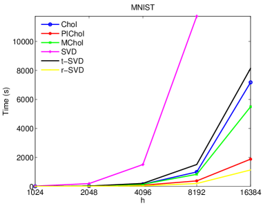
Figure 6: Times (in seconds) of the $6$ considered algorithm, summed over all cross validation folds, as a function of $h$ on MNIST data.

	MNIST	COIL	Caltech	Caltech
		-100	-101	-256
Chol	718	691	706	686
PIChol	188	167	169	174
MChol	550	235	545	527
SVD	9415	3489	9060	9823
t-SVD	815	858	1078	1318
r-SVD	1140	67	78	111

Table 3: Time taken by the six algorithms when $h=16384$ per cross validation fold. All times are reported in seconds.

Figure 6 and Table 3 show the timing results of the Cholesky and SVD-based algorithms. It can be observed that the PIChol has significant speedups over Chol and MChol. Moreover, the SVD and t-SVD are always the slowest. Finally, r-SVD is always the fastest algorithm; however, as we will see in the holdout-error results, r-SVD does not give any useful conclusions for the optimal $\lambda$ value. Figure 6 shows the timings for the MNIST data. We obtained similar timing trends for all the four data-sets we used.

6.5 Hold-out Errors

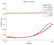
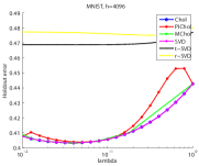
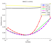
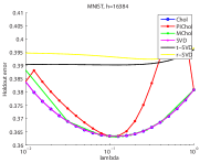
Figure 7: Hold-out errors for the six algorithms as a function of $\lambda$ on the MNIST data.

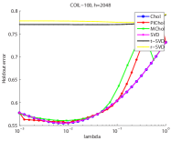
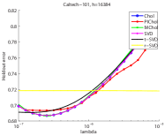
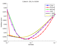
Figure 8: a, b– Hold-out errors for the six algorithms as a function of $\lambda$ on the COIL-100 dataset for projection dimensions of $2048$ and $4096$ respectively. c, d– Hold-out errors for the six algorithms as a function of $\lambda$ on Caltech 101 and Caltech 256.

	MNIST		COIL-100		Caltech-101		Caltech-256
	Minimum ho-	Selected	Minimum ho-	Selected	Minimum ho-	Selected	Minimum ho-	Selected
	ldout error	$\lambda$	ldout error	$\lambda$	ldout error	$\lambda$	ldout error	$\lambda$
Chol	0.3633	0.1259	0.4507	0.01	0.6869	2.51e-7	0.9422	0.0063
PIChol	0.3634	0.1	0.4507	0.01	0.6934	2.51e-7	0.9421	0.0079
MChol	0.3633	0.1186	0.4506	0.009	0.6869	2.51e-7	0.9422	0.0057
SVD	0.3633	0.1259	0.4507	0.01	0.6869	2.51e-7	0.9422	0.0063
t-SVD	0.3903	0.1259	0.6812	0.0794	0.6908	1.58e-7	0.9443	0.0032
r-SVD	0.3925	0.3162	0.6874	0.1995	0.7180	1.0e-5	0.9444	0.004

Table 4: The minimum hold-out error and the selected $\lambda$ value for the six considered algorithms on four datasets.

Figure 7 shows the hold-out errors obtained for MNIST data when projected to $2048$, $4096$, $8192$, and $16384$ dimensions respectively. Similarly, Figure 8-a and b show the hold-out errors for COIL-100 data for $2048$ and $4096$ dimensions, while Figure 8-c and d show hold-out errors for Caltech 101 and Caltech 256 datasets for $16384$ dimensions each. Table 4 shows the minimum hold-out error and the selected $\lambda$ value for each algorithm on all the four data sets. Figure 9 shows the error in the selected $\lambda$’s for Chol, PIChol, and MChol as a function of running time on COIL-100 and Caltech-101 datasets.

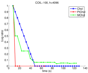
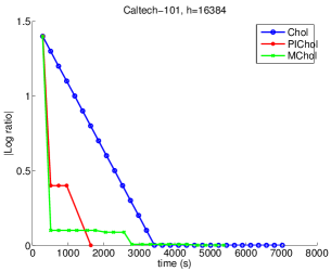
Figure 9: Absolute value of the logarithmic ratio between the selected $\lambda$ and the optimal $\lambda$ as Chol, PIChol, and MChol proceed in time.

It can be observed that PIChol closely approximates the behavior of Chol and SVD. The approximation for $h=2048,4096$ is better than that for $h=8192,16384$; however, we notice that for the latter two cases with larger $h$, the approximation quality of PIChol is satisfactory when $\lambda$ is close to the optimal $\lambda$ value. This phenomenon justifies the effectiveness of our framework for choosing the optimal regularization parameter. From Table 4, we can see that PIChol and MChol give consistently close approximation of the optimal $\lambda$ value; however, from Figure 9 and Table 3, we conclude that MChol takes much longer time than PIChol to reach the same level of accuracy. Though t-SVD and r-SVD might be faster, they generate very poor approximation of the true hold-out error and the optimal $\lambda$ value, and therefore their efficiency advantage is of little practical use.

Note that another potential way of finding the optimal $\lambda$ from a sparsely sampled set of $\lambda$ values is to interpolate the hold-out error itself based on the hold-out errors computed for the sparsely sampled set. We empirically found that this approach did not yield a good fit to the true hold-out error curve. In the interest of space, we show the detailed results for this scheme (named as PINRMSE) in the supplementary materials.

An alternative way to find the optimal $\lambda$ that corresponds to the minimal hold-out error is by interpolating a sparse set of hold-out errors directly. We refer to this approach as PINRMSE. More precisely, PINRMSE is equivalent to replacing the $g\times\textrm{D}$ matrix T in Algorithm 1 with a $g\times 1$ vector t, where the entries in t are the hold-out errors that correspond to the sparsely sampled $\lambda$ values. We then interpolate the hold-out errors for the dense set of $\lambda$ values.

Figure 10 demonstrates that PINRMSE often gives substantially worse interpolation accuracy than PIChol and could therefore result in dramatically wrong $\lambda$ values. For instance, while PINRMSE achieved the true optimal $\lambda$’s on COIL-100 and Caltech-256 data sets, it selected $\lambda$s that are significantly far away from the optimal values on MNIST and Caltech-101 data sets. On the contrary, PIChol consistently selected the correct $\lambda$’s on all the data sets.

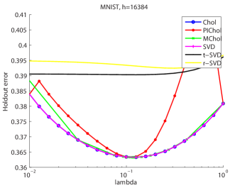
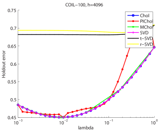
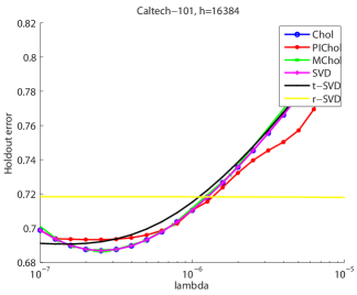
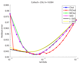
Figure 10: Comparisons between PINRMSE and Chol, PIChol, SVD, t-SVD, r-SVD. Both PINRMSE and PIChol use the parameters $g=4$ and $r=2$ in the context of Algorithm 1.

6.6 Normalized Root Mean Squared Error

Figure 11 shows the normalized root mean squared error (NRMSE) for least-squares fit of PIChol on MNIST. Similar trends hold for all considered data-sets. Recall that naively using the mean of target variable implies NRMSE of $1$. Our maximum NRMSE of $0.0457$ hence implies quite high interpolation accuracy.

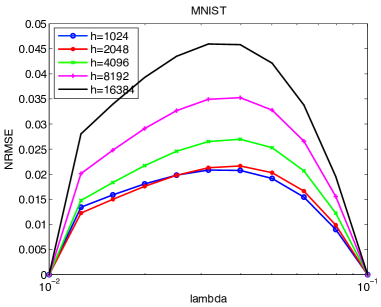
Figure 11: NRMSE for $pi$Cholesky on MNIST as a function of regularization parameter $\lambda$.

7 Conclusions & Future Work

In this work, we proposed an efficient way to densely interpolate Cholesky factors of Hessian matrix for a sparse set of $\lambda$ values. This idea enabled us to exhaustively explore the space of $\lambda$ values, and therefore optimally minimize the hold-out error while incurring only a fraction of the cost of exact cross-validation. Our key observation was that Cholesky factors for different $\lambda$ values tend to lie on smooth curves that can be approximated accurately using polynomial functions. We theoretically proved this observation and provided an error bound for our approximation. We presented a framework to learn these multiple polynomial functions simultaneously, and proposed solutions for its efficiency challenges. In particular, we proposed a recursive block Cholesky vectorization strategy for efficient vectorization of a triangular matrix. This is a general scheme and is not restricted to the scope of this work.

Currently, we apply the learned polynomial functions within a particular validation fold. Going forward, we intend to use these functions to warm-start the learning process in a different fold. This would reduce the number of exact Cholesky factors required in a fold, further improving our performance. We also intend to apply our framework to speed-up regularization in other problems, e.g., matrix completion [29] and sparse coding [30].

References

- [1] Ethem Alpaydin. Introduction to machine learning. MIT press, 2004.
- [2] S. Brenner and R. Scott. The Mathematical Theory of Finite Element Methods. Springer, 3rd edition, 2007.
- [3] James R Bunch and Christopher P Nielsen. Updating the singular value decomposition. Numerische Mathematik, 31(2):111–129, 1978.
- [4] Gavin C Cawley and Nicola LC Talbot. Fast exact leave-one-out cross-validation of sparse least-squares support vector machines. Neural networks, 17(10):1467–1475, 2004.
- [5] Thomas G. Dietterich and Ghulum Bakiri. Solving multiclass learning problems via error-correcting output codes. arXiv preprint cs/9501101, 1995.
- [6] Bradley Efron, Trevor Hastie, Iain Johnstone, Robert Tibshirani, et al. Least angle regression. The Annals of statistics, 32(2):407–499, 2004.
- [7] Li Fei-Fei, Rob Fergus, and Pietro Perona. Learning generative visual models from few training examples: An incremental bayesian approach tested on 101 object categories. CVIU, 2007.
- [8] Gene Golub and William Kahan. Calculating the singular values and pseudo-inverse of a matrix. Journal of the Society for Industrial & Applied Mathematics, Series B: Numerical Analysis, 2(2):205–224, 1965.
- [9] Gene H Golub and Charles F Van Loan. Matrix computations. Johns Hopkins University Press, 2012.
- [10] Gregory Griffin, Alex Holub, and Pietro Perona. Caltech-256 object category dataset. 2007.
- [11] Ming Gu and Stanley C Eisenstat. Downdating the singular value decomposition. SIAM Journal on Matrix Analysis and Applications, 16(3):793–810, 1995.
- [12] William W Hager. Updating the inverse of a matrix. SIAM review, 31(2):221–239, 1989.
- [13] Nathan Halko, Per-Gunnar Martinsson, and Joel A Tropp. Finding structure with randomness: Probabilistic algorithms for constructing approximate matrix decompositions. SIAM, 53(2):217–288, 2011.
- [14] Per Christian Hansen. The truncatedsvd as a method for regularization. BIT Numerical Mathematics, 27(4):534–553, 1987.
- [15] Roger A Horn and Charles R Johnson. Matrix analysis. Cambridge university press, 2012.
- [16] Michael Kaess, Hordur Johannsson, Richard Roberts, Viorela Ila, John Leonard, and Frank Dellaert. isam2: Incremental smoothing and mapping with fluid relinearization and incremental variable reordering. In ICRA, pages 3281–3288. IEEE, 2011.
- [17] Purushottam Kar and Harish Karnick. Random feature maps for dot product kernels. Journal of Machine Learning Research, 22:583–591, 2012.
- [18] Seung-Jean Kim, Kwangmoo Koh, Michael Lustig, Stephen Boyd, and Dimitry Gorinevsky. An interior-point method for large-scale l1regularized least squares. STSP, 2007.
- [19] Ioannis Koutis, Gary L Miller, and Richard Peng. A fast solver for a class of linear systems. Communications of the ACM, 55(10):99–107, 2012.
- [20] Svetlana Lazebnik, Cordelia Schmid, and Jean Ponce. Beyond bags of features: Spatial pyramid matching for recognizing natural scene categories. In CVPR, 2006.
- [21] Quoc Le, Tamas Sarlos, and Alexander Smola. Fastfood-computing hilbert space expansions in loglinear time. In ICML, pages 244–252, 2013.
- [22] Yann LeCun and Corinna Cortes. The mnist database of handwritten digits, 1998.
- [23] John Mandel. Use of the singular value decomposition in regression analysis. The American Statistician, 36(1):15–24, 1982.
- [24] Jerrold E. Marsden, Tudor Ratiu, and Ralph Abraham. Manifolds, Tensor Analysis, and Applications. Springer-Verlag, 3rd edition, 2001.
- [25] S. A. Nene, S. K. Nayar, and H. Murase. Columbia object image library (coil-100). Technical Report CUCS-006-96, Columbia University, 1996.
- [26] Kaare Brandt Petersen and Michael Syskind Pedersen. The Matrix Cookbook. Technical University of Denmark, 2012.
- [27] Yousef Saad. Iterative methods for sparse linear systems. Siam, 2003.
- [28] B. Schlkopf, C. J. C. Burges, and A. J. Smola, editors. Advances in Kernel Methods: Support Vector Learning. MIT Press, 1999.
- [29] Nathan Srebro, Jason Rennie, and Tommi Jaakkola. Maximum margin matrix factorization. In Advances in Neural Information Processing Systems 17, pages 1329–1336, 2004.
- [30] Arthur Szlam, Zhaohui Guo, and Stanley Osher. A split bregman method for non-negative sparsity penalized least squares with applications to hyperspectral demixing. In ICIP, 2010.
- [31] Andrey Nikolayevich Tikhonov. On the stability of inverse problems. In Dokl. Akad. Nauk SSSR, volume 39, 1943.
- [32] Henk A Van der Vorst. Iterative Krylov methods for large linear systems, volume 13. Cambridge University Press, 2003.