LPT-ORSAY/14-17
Analyticity of $\eta\pi$ isospin-violating form factors and the $\tau\to\eta\pi\nu$ second-class decay

Abstract

We consider the evaluation of the $\eta\pi$ isospin-violating vector and scalar form factors relying on a systematic application of analyticity and unitarity, combined with chiral expansion results. It is argued that the usual analyticity properties do hold (i.e. no anomalous thresholds are present) in spite of the instability of the $\eta$ meson in QCD. Unitarity relates the vector form factor to the $\eta\pi\to\pi\pi$ amplitude: we exploit progress in formulating and solving the Khuri-Treiman equations for $\eta\to 3\pi$ and in experimental measurements of the Dalitz plot parameters to evaluate the shape of the $\rho$-meson peak. Observing this peak in the energy distribution of the $\tau\to\eta\pi\nu$ decay would be a background-free signature of a second-class amplitude. The scalar form factor is also estimated from a phase dispersive representation using a plausible model for the $\eta\pi$ elastic scattering $S$-wave phase shift and a sum rule constraint in the inelastic region. We indicate how a possibly exotic nature of the $a_{0}(980)$ scalar meson manifests itself in a dispersive approach. A remark is finally made on a second-class amplitude in the $\tau\to\pi\pi\nu$ decay.

1 Introduction

Isospin-breaking phenomena involving light pseudoscalar mesons are particularly interesting probes of the three flavour chiral expansion as they are driven by the parameter

$$\epsilon={\sqrt{3}(m_{d}-m_{u})\over 4(m_{s}-(m_{u}+m_{d})/2)}$$ (1)

which involves the three light-quark masses. One of the major goals of non-perturbative approaches to QCD is to arrive at an accurate determination of the light-quark masses. One issue in the direct determination of $\epsilon$ from the very precisely known difference between the masses of the charged and the neutral kaon is to properly evaluate the electromagnetic contribution to this difference. At leading chiral order, it is given by Dashen’s low-energy theorem [1]. There are, however, possible substantial corrections from next-to-leading $O(e^{2}m_{s})$ effects which suggests to explore, in parallel, other isospin-violating processes.

In this respect, the $\eta\to 3\pi$ decay amplitude is of particular interest since electromagnetic contributions are absent at leading order [2] and found to be rather small at next-to-leading order (NLO) [3, 4, 5]. Furthermore, there has been considerable progress, on the experimental side, in the precision of the measurements of the Dalitz plot parameters for both the $\eta\to 3\pi^{0}$ amplitude[6, 7, 8, 9] and the $\eta\to\pi^{+}\pi^{-}\pi^{0}$ amplitude[10]. There is a price to pay, however, in that the chiral expansion has an inherently slow convergence in the treatment of final-state interactions, e.g. in the NLO expression of the $\eta\to 3\pi$ amplitude [11], $\pi\pi$ rescattering is treated only at leading chiral order. The amplitude has now been computed to NNLO in chiral perturbation theory (ChPT) [12]. A partly analytic representation of the $\pi\pi$ rescattering part at NNLO, accounting for some effects of higher order, was obtained in ref. [13]. A treatment of rescattering in the framework of non-relativistic effective field theory has been discussed in ref. [14]. An alternative approach is to combine the chiral expansion with a more general representation which encodes exact unitarity, analyticity and crossing symmetry [15]. A rigorous framework was proposed by Khuri and Treiman (KT) [16] who derived a set of integral equations for the analogous $K\to 3\pi$ problem. Application to the $\eta\to 3\pi$ amplitude was first discussed in ref. [17]. The KT equations were more recently generalised to account for both $S$ and $P$-wave elastic rescattering [18, 19] and numerical solutions were constructed. Updates of these analyses, which take into account the recent experimental data, have been presented [20, 21, 22].

This progress have motivated us to reconsider the problem of evaluating the $\eta\pi$ isospin-violating vector and scalar form factors exploiting, as systematically as possible, their analyticity properties and matching with chiral NLO calculations [23, 24]. The vector form factor, in particular, probes the $\eta\pi\to\pi\pi$ amplitude, via unitarity, in a kinematical region different from that of the decay, but where the KT equations should still be applicable. These two form factors are measurable, in principle, from the $\tau\to\eta\pi\nu$ decay mode. This mode, being forbidden in the isospin-symmetric limit, is a clean example of the “second-class currents” as introduced by Weinberg [25], which are yet to be discovered experimentally. An upper bound on the branching fraction, $B_{\eta\pi}<1.4\times 10^{-4}$, was obtained by the CLEO collaboration[26] which was slightly improved to $B_{\eta\pi}<9.9\times 10^{-5}$ by Babar [27]. The Belle collaboration has quoted $B_{\eta\pi}<7.3\times 10^{-5}$ as a preliminary result [28] which, however, was not subsequently confirmed. Theoretical estimates for this branching fraction [29, 30, 31, 23, 32, 33, 34] yield values in the range $10^{-6}$ to $10^{-5}$, which do not seem so small as compared to the number of $\tau$ pairs available at Babar: $N_{\tau}\simeq 4.3\times 10^{8}$ or Belle $N_{\tau}\simeq 9.0\times 10^{8}$. One difficulty faced by the $B$ factories was that a substantial number of $\eta\pi$ pairs were produced from background modes, like $\tau^{-}\to\eta\pi^{-}\pi^{0}\nu$, which have to be subtracted. A drastic reduction of this background should be possible at $\tau$-charm factories [35, 36] which could make detailed measurements of the $\eta\pi$ mode possible. An increase in the luminosity by a factor of fifty is expected at Belle II [37].

Here, we will consider not only the integrated $\tau\to\eta\pi\nu_{\tau}$ branching fraction but also the detailed dependence as a function of the $\eta\pi$ invariant mass. This dependence carries nontrivial dynamical information. Close to $s=0$ it can be related, via ChPT, to the isospin-breaking quark mass ratio $\epsilon$ while, at higher energy, the shape of the $\rho$ resonance peak in the vector form factor can be related to $\eta\to 3\pi$ decay properties. From an experimental point of view, the observation of the $\rho$ peak would be a background-free signal of a second-class amplitude. A peak at the $a_{0}(980)$ mass is also expected from the scalar form factor. As was noted long ago [38], the mode $\tau\to\eta\pi\nu$ probes the “nature” of the scalar meson $a_{0}(980)$ in a clean way via its coupling to the $\bar{u}d$ operator.

The $\eta\pi$ scalar form factor has a potential for constraining extensions of the Standard Model which contain charged Higgs bosons. For illustration, in the two-Higgs model proposed in ref. [39] , the energy dependence of the form factor is modified as follows,

$$f^{\eta\pi}_{0}(s)=\left.f^{\eta\pi}_{0}\right(s)|_{SM}\left(1-{\zeta^{*}_{\tau}(\zeta_{u}m_{u}-\zeta_{d}m_{d})\over m_{u}-m_{d}}\times{s\over m^{2}_{H^{+}}}\right)$$ (2)

where the $\zeta$’s are coupling constants. The influence of the charged Higgs in this form factor could be enhanced because of the $m_{u}-m_{d}$ denominator, depending on the relative sign and size of $\zeta_{u}$, $\zeta_{d}$. The constraints which are already available (specifically from $B\to\tau\nu$) are not so stringent: $|\zeta_{l}\zeta_{d}/m^{2}_{H^{+}}|<0.1$ $\hbox{GeV}^{-2}$ [40]. In order to derive a similar level of constraint, one should be able to evaluate $f^{\eta\pi}_{0}$ in the Standard Model (and also be able to measure it, of course) with a precision of $\simeq 20\%$ at $s=1\ \hbox{GeV}^{2}$.

The plan of the paper is as follows. After introducing some basic formulae and notation, we list the contributions from the light two-meson states to the unitarity relations of the two form factors. We also discuss contributions with one photon. Then, we recall the main results from the NLO ChPT calculations [23, 24]: the values of the form factors at $s=0$ and their first derivatives will be used as input in the dispersive representations. In order to derive these, it is important to check the possible presence of anomalous thresholds, since the $\eta$ meson is unstable: we present arguments that they are actually absent. We then discuss the dispersive evaluation of the vector form factor using as input $\pi\eta\to\pi\pi$ amplitudes satisfying the KT equations and constrained by experimental data in the physical decay region. Finally, we estimate the scalar form factor from a phase dispersive representation, using a modelling of $\eta\pi\to\eta\pi$ elastic scattering borrowed from ref. [41].

2 Definitions and basic unitarity relations

The semi-leptonic weak decay amplitudes $\tau\to\eta\pi\nu$ and $\eta\to l\pi\nu$ (with $l=e,\mu$) are induced by the usual Fermi Lagrangian

$${\cal L}_{F}=-{G_{F}V_{ud}\over\sqrt{2}}\left[\bar{u}\gamma^{\mu}(1-\gamma^{5})d\times\bar{l}\gamma_{\mu}(1-\gamma^{5})\nu_{l}+h.c.\right]\ .$$ (3)

The $\eta\pi$ matrix element of the charged vector current is expressed in terms of two form factors (we follow the same notation as ref. [23] except that we call the $\eta\pi$ invariant mass squared $s$ instead of $t$),

$${\mathrel{\hbox{$\langle$}\kern-1.16667pt\lower 8.25005pt\hbox{$\scriptstyle{out}$}\kern-3.57404pt}\eta(p_{\eta})\pi^{+}(p_{\pi})|j_{\mu}^{ud}(0)|0\rangle}=-\sqrt{2}\left[f_{+}^{\eta\pi}(s)(p_{\eta}-p_{\pi^{+}})_{\mu}+f_{-}^{\eta\pi}(s)(p_{\eta}+p_{\pi^{+}})_{\mu}\right]\$$ (4)

with

$$j_{\mu}^{ud}(x)=\bar{u}(x)\gamma_{\mu}d(x),\quad s=(p_{\eta}+p_{\pi})^{2}\ .$$ (5)

When writing unitarity relations it is convenient to introduce the scalar form factor $f_{0}^{\eta\pi}(s)$ instead of $f_{-}^{\eta\pi}(s)$

$$f_{0}^{\eta\pi}(s)=f_{+}^{\eta\pi}(s)+{s\over\Delta_{\eta\pi}}f_{-}^{\eta\pi}(s),\quad\Delta_{PQ}=m_{P}^{2}-m_{Q}^{2}$$ (6)

The expression for the differential decay width of the $\tau$ lepton which derives from the Fermi Lagrangian (3) and the definition of the form factors (4) then reads

$${d\Gamma_{\tau\to\eta\pi\nu_{\tau}}\over ds}={G_{F}^{2}V_{ud}^{2}S_{EW}\,m_{\tau}^{3}\over 384\,\pi^{3}}{\sqrt{\lambda_{\eta\pi}{(s)}}\over s^{3}}\left(1-{s\over m_{\tau}^{2}}\right)^{2}$$ (7)

$$\quad\quad\times\bigg{\{}|f^{\eta\pi}_{+}(s)|^{2}\,\lambda_{\eta\pi}{(s)}\left(1+{2s\over m_{\tau}^{2}}\right)+3|f^{\eta\pi}_{0}(s)|^{2}\Delta_{\eta\pi}^{2}\bigg{\}}$$

where $S_{EW}$ is the logarithmically enhanced universal radiative correction factor [42] ($S_{EW}=1.0201$ [43]) and

$$\lambda_{PQ}(s)=\lambda(s,m_{P}^{2},m_{Q}^{2})\ ,$$ (8)

$\lambda$ being the Källén function $\lambda(x,y,z)=x^{2}+y^{2}+z^{2}-2(xy+yz+xz)$. For the physical $\tau$ decay, the variable $s$ lies in the range $(m_{\eta}+m_{\pi})^{2}\leq s\leq m_{\tau}^{2}$. The analogous formula for the differential decay of the $\eta$, $\eta\to l^{\pm}\pi^{\mp}\nu_{l}$ with $l=e$ or $l=\mu$ reads

$${d\Gamma_{\eta\to l\pi\nu_{l}}\over ds}={G_{F}^{2}V_{ud}^{2}S_{EW}\over 192\pi^{3}}{\sqrt{\lambda_{\eta\pi}{(s)}}\over m_{\eta}^{3}}\left(1-{m_{l}^{2}\over s}\right)^{2}$$

$$\quad\quad\times\left\{|f^{\eta\pi}_{+}(s)|^{2}\,\lambda_{\eta\pi}{(s)}\left(2+{m_{l}^{2}\over s}\right)+3|f^{\eta\pi}_{0}(s)|^{2}\Delta_{\eta\pi}^{2}{m_{l}^{2}\over s}\right\}\ .$$ (9)

In this case, the variable $s$ is restricted to the range $m_{l}^{2}\leq s\leq(m_{\eta}-m_{\pi})^{2}$.

2.1 Unitarity relations for $f^{\eta\pi}_{+}(s)$

We consider the $\eta\pi^{+}$ center-of-mass system and choose the $z$-axis along the three-momentum of the $\eta$ meson. The vector form factor is easily seen to be proportional to the matrix element of the third component of the vector current in this frame

$${\mathrel{\hbox{$\langle$}\kern-1.16667pt\lower 8.25005pt\hbox{$\scriptstyle{out}$}\kern-3.57404pt}\eta(p_{\eta})\pi^{+}(p_{\pi})|j_{3}^{ud}(0)|0\rangle}=-2\sqrt{2}q_{\eta\pi}(s)\,f^{\eta\pi}_{+}(s)\ ,$$ (10)

where $q_{\eta\pi}(s)$ is the center-of-mass momentum. The form factor $f^{\eta\pi}_{+}(s)$ can be defined as an analytic function of $s$ with a cut along the positive real axis starting at $s_{th}=4m_{\pi}^{2}$ (see the discussion about the absence of anomalous thresholds in sec. 4 below). The discontinuity across the cut has the form of a generalised unitarity relation and is given as a sum over a complete set of states,

$$-2\sqrt{2}\,q_{\eta\pi}(s)\,\hbox{disc}[f^{\eta\pi}_{+}(s)]={1\over 2}\sum_{n}T^{*}_{\eta\pi^{+}\to n}\times{\mathrel{\hbox{$\langle$}\kern-1.16667pt\lower 8.25005pt\hbox{$\scriptstyle{out}$}\kern-3.57404pt}n|j_{3}^{ud}(0)|0\rangle}\ .$$ (11)

with

$$\hbox{disc}[f^{\eta\pi}_{+}(s)]\equiv{f^{\eta\pi}_{+}(s+i\epsilon)-f^{\eta\pi}_{+}(s-i\epsilon)\over 2i}\ .$$ (12)

The lightest state contributing to the unitarity relation is $n=\pi^{0}\pi^{+}$ with angular momentum $l=1$. The next-to-lightest contribution is from four pion states $n=\pi^{0}\pi^{+}\pi\pi$. However, we expect such contributions not to be effectively relevant below 1 GeV because of phase space suppression and we will ignore them here. Let us consider successively the contributions from the lightest two-body states $n=\pi^{0}\pi^{+}$, $n=\eta\pi^{+}$ and $n=\bar{K}^{0}K^{+}$

• $n=\pi^{0}\pi^{+}$:
  The $\pi^{0}\pi^{+}$ matrix element of the vector current,

  $${\mathrel{\hbox{$\langle$}\kern-1.16667pt\lower 8.25005pt\hbox{$\scriptstyle{out}$}\kern-3.57404pt}\pi^{0}\pi^{+}|j_{\mu}^{ud}|0\rangle}=\sqrt{2}\left[F_{V}^{\pi}(s)(p_{{\pi^{0}}}-p_{{\pi^{+}}})_{\mu}+F_{-}^{\pi}(s)(p_{{\pi^{0}}}+p_{{\pi^{+}}})_{\mu}\right]\ ,$$ (13)

  involves two form factors since $m_{\pi^{+}}\neq m_{\pi^{0}}$. The unitarity relation for $f_{+}^{\eta\pi}$ involves only the vector form factor, $F_{V}^{\pi}(s)$. Using eq. (11), we can write the $\pi\pi$ contribution in the unitarity relation as follows

  $$\hbox{disc}\left[f^{\eta\pi}_{+}(s)\right]_{\pi\pi}=-\theta(s-4m_{\pi}^{2}){s-4m_{\pi}^{2}\over 16\pi\,\sqrt{\lambda_{\eta\pi}{(s)}}}\,F_{V}^{\pi}(s)$$

  $$\phantom{\left.\hbox{disc}f^{\eta\pi}_{+}(s)\right|_{\pi\pi}}\quad\times{1\over 2}\int_{-1}^{1}dzz\,T^{*}_{\pi^{0}\pi^{+}\to\eta\pi^{+}}(s,t,u)\ ,$$ (14)

  where $z=\cos\theta$, $\theta$ being the scattering angle in the center-of-mass system. We expect this contribution to be important below 1 GeV, because of the presence of the $\rho(770)$ resonance.

• $n=\eta\pi^{+}$
  Next, the contribution from the $\eta\pi$ state to the unitarity relation reads

  $$\hbox{disc}\left[f^{\eta\pi}_{+}(s)\right]_{\eta\pi}=\theta(s-(m_{\eta}+m_{\pi})^{2}){\sqrt{\lambda_{\eta\pi}{(s)}}\over 16\pi s}f^{\eta\pi}_{+}(s)$$

  $$\phantom{\hbox{disc}\left[f^{\eta\pi}_{+}(s)\right]_{\eta\pi}}\times{1\over 2}\int_{-1}^{1}dz\,z\,T^{*}_{\eta\pi^{+}\to\eta\pi^{+}}(s,t,u)$$ (15)

  This contribution involves the $\eta\pi\to\eta\pi$ amplitude projected on the $P$-wave. The quantum numbers of the state $(\eta\pi)_{l=1}$ are exotic: $J^{PC}=1^{-+}$. We expect the $(\eta\pi\to\eta\pi)_{l=1}$ amplitude to be very small below 1 GeV. This is borne out by the $\eta\pi$ scattering model proposed in ref. [41], which predicts that the $P$-wave phase shift is of the order of $-1^{\circ}$ at 1 GeV.

• $n={\bar{K}^{0}}{K^{+}}$
  Finally, let us write the contribution of the ${\bar{K}^{0}}{K^{+}}$ state in the unitarity relation, which is useful for comparing with the chiral calculation. In this case, the kaon vector form factor appears, defined from

  $${\mathrel{\hbox{$\langle$}\kern-1.16667pt\lower 8.25005pt\hbox{$\scriptstyle{out}$}\kern-3.57404pt}{\bar{K}^{0}K^{+}}|j_{\mu}^{ud}|0\rangle}=-\left[F_{V}^{K}(s)(p_{{\bar{K}^{0}}}-p_{{K^{+}}})_{\mu}+F_{-}^{K}(s)(p_{{\bar{K}^{0}}}+p_{{K^{+}}})_{\mu}\right]\ .$$ (16)

  The corresponding contribution in the unitarity relation reads

  $$\hbox{disc}\left[f^{\eta\pi}_{+}(s)\right]_{\bar{K}K}=\theta(s-4m_{K}^{2}){s-4m_{K}^{2}\over 16\pi\sqrt{2}\,\sqrt{\lambda_{\eta\pi}{(s)}}}\,F_{V}^{K}(s)$$

  $$\phantom{\hbox{disc}\left[f^{\eta\pi}_{+}(s)\right]_{\bar{K}K}}\times{1\over 2}\int_{-1}^{1}dzzT^{*}_{{\bar{K}^{0}K^{+}}\to\eta\pi^{+}}(s,t,u)\ .$$ (17)

  In the above expression, isospin breaking is contained in the amplitude ${{\bar{K}^{0}K^{+}}\to\eta\pi^{+}}$ projected on the $P$-wave. Let us recall the reason: since $G{|K^{+}\rangle}={|\bar{K}_{0}\rangle}$, $G{|\bar{K}_{0}\rangle}=-{|K^{+}\rangle}$ one has $G|\bar{K}_{0}K^{+}\rangle=(-1)^{l+1}|\bar{K}_{0}K^{+}\rangle$. Since $\eta\pi$ has G-parity $-1$, this implies that the partial-wave amplitudes $({\bar{K}^{0}K^{+}}\to\eta\pi^{+})_{l}$ with odd angular momentum $l$ vanish in the isospin limit.

2.2 Unitarity relations for $f^{\eta\pi}_{0}(s)$

Unitarity relations for the scalar form factor can be derived in exactly the same way as above noticing that, in the center-of-mass frame, the matrix element of the zeroth component of the vector current is proportional to $f^{\eta\pi}_{0}$,

$${\mathrel{\hbox{$\langle$}\kern-1.16667pt\lower 8.25005pt\hbox{$\scriptstyle{out}$}\kern-3.57404pt}\eta(p_{\eta})\pi^{+}(p_{\pi})|j^{ud}_{0}(0)|0\rangle}=-{\sqrt{2}\Delta_{\eta\pi}\over\sqrt{s}}\,f_{0}^{\eta\pi}(s)$$ (18)

One can then derive a relation for the discontinuity along the cut, analogous to eq. (11),

$$-{\sqrt{2}\Delta_{\eta\pi}\over\sqrt{s}}\,\hbox{disc}[f_{0}^{\eta\pi}(s)]={1\over 2}\sum_{n}T^{*}_{\eta\pi^{+}\to n}\times{\mathrel{\hbox{$\langle$}\kern-1.16667pt\lower 8.25005pt\hbox{$\scriptstyle{out}$}\kern-3.57404pt}n|j_{0}^{ud}(0)|0\rangle}\ .$$ (19)

As before, let us consider the contributions from the lightest two-particle states $\pi\pi$, $\pi\eta$ and $K\bar{K}$.

• $n=\pi^{0}\pi^{+}$:
  Introducing a scalar pion form factor from eq. (13)

  $$f_{0}^{\pi\pi}(s)=F_{V}^{\pi}(s)+{s\over\Delta_{\pi^{0}\pi^{+}}}F_{-}^{\pi}(s)$$ (20)

  one derives that

  $$\hbox{disc}\left[f^{\eta\pi}_{0}\right]_{\pi^{0}\pi^{+}}=-\theta(s-4m_{\pi}^{2}){\sqrt{s-4m_{\pi}^{2}}\over 16\pi\sqrt{s}}{\Delta_{\pi^{0}\pi^{+}}\over\Delta_{\eta\pi^{+}}}f_{0}^{\pi\pi}(s)$$

  $$\phantom{\hbox{disc}\left[f^{\eta\pi}_{0}\right]_{\pi^{0}\pi^{+}}}\times{1\over 2}\int_{-1}^{1}dz\,T^{*}_{\eta\pi^{+}\to\pi^{0}\pi^{+}}(s,t,u)\ .$$ (21)

  This contribution involves a product of two isospin-breaking terms ($\Delta_{\pi^{0}\pi^{+}}$ and $T^{*}_{\eta\pi^{+}\to\pi^{0}\pi^{+}}$) and thus must be negligibly small in practice.

• $n=\eta\pi^{+}$:
  The contribution from the $\eta\pi^{+}$ states to the unitarity relation reads

  $$\hbox{disc}\left[f^{\eta\pi}_{0}\right]_{\eta\pi}=\theta(s-(m_{\eta}+m_{\pi})^{2})){\sqrt{\lambda_{\eta\pi}{(s)}}\over 16\pi s}f^{\eta\pi}_{0}(s)$$

  $$\phantom{\hbox{disc}\left[f^{\eta\pi}_{0}\right]_{\eta\pi}}\times{1\over 2}\int_{-1}^{1}dz\,T^{*}_{\eta\pi^{+}\to\eta\pi^{+}}(s,t,u)\ .$$ (22)

  It has a form similar to eq. (b)) for the vector form factor except that it involves the $\eta\pi\to\eta\pi$ amplitude projected on the $S$-wave instead of the $P$-wave. This contribution is enhanced by the presence of the $a_{0}(980)$ resonance and thus must be the dominating one below 1 GeV.

• $n={\bar{K}^{0}}{K^{+}}$:
  Finally, the contribution from ${\bar{K}^{0}}{K^{+}}$ involves the corresponding scalar form factor

  $$f_{0}^{{\bar{K}^{0}}{K^{+}}}(s)\equiv F_{V}^{K}(s)+{s\over\Delta_{{\bar{K}^{0}}{K^{+}}}}F_{-}^{K}(s)$$ (23)

  and it has the following expression

  $$\hbox{disc}\left[f^{\eta\pi}_{0}\right]_{{\bar{K}^{0}}{K^{+}}}(s)=\theta(s-4m_{K}^{2}){\sqrt{s-4m_{K}^{2}}\over 16\pi\sqrt{s}}{\Delta_{{\bar{K}^{0}}{K^{+}}}\over\sqrt{2}\Delta_{\eta\pi}}f_{0}^{{\bar{K}^{0}}{K^{+}}}(s)$$

  $$\phantom{\hbox{disc}\left[f^{\eta\pi}_{0}\right]_{{\bar{K}^{0}}{K^{+}}}(s)}\times{1\over 2}\int_{-1}^{1}dz\,T^{*}_{\eta\pi^{+}\to{\bar{K}^{0}}{K^{+}}}(s,t,u)\ .$$ (24)

  As compared to the analogous contribution for $f^{\eta\pi}_{+}$, the relation (c)) involves the $\eta\pi^{+}\to{\bar{K}^{0}}{K^{+}}$ amplitude projected on the $S$-wave, which is isospin conserving. Isospin breaking is contained in the mass difference factor $\Delta_{{\bar{K}^{0}}{K^{+}}}$.

2.3 Some electromagnetic contributions to the unitarity relations

In the unitarity equations discussed above, we have considered only hadronic states in the sums over $n$. Since we are studying isospin-breaking form factors, electromagnetic contributions are present and, at order $e^{2}$ one should also consider states involving one photon. Note that EM contributions have already appeared, e.g. in eqs. (a)), (c)) which are proportional to the mass differences $m_{\pi^{0}}^{2}-m_{\pi^{+}}^{2}$ (which is mainly electromagnetic) and $m_{\bar{K}^{0}}^{2}-m_{K^{+}}^{2}$ (which is partly of electromagnetic origin). These contributions are dominant in the chiral counting; they are included in the NLO chiral expressions. We will not discuss EM contributions in their full generality here and simply mention the contributions of the two lightest states $n=\gamma\pi$ and $n=\gamma\pi\pi$ in the unitarity relations:

• $n=\gamma\pi$
  The $\gamma\pi$ matrix element of the vector current can be expressed in terms of one form factor

  $${\langle\gamma(\lambda)\pi^{+}|j_{\mu}^{ud}(0)|0\rangle}=eF_{V}^{\pi\gamma}(s)\,\varepsilon_{\mu}[e_{\gamma}(\lambda),p_{\gamma},p_{\pi^{+}}]$$ (25)

  where $e_{\gamma}$ is the polarisation vector of the photon. At leading order in the chiral expansion, the value of this form factor at $s=0$ is given by the anomaly

  $$\left.F_{V}^{\gamma\pi}(0)\right|_{LO}={\sqrt{2}N_{c}\over 24\pi^{2}F_{\pi}^{2}}\ .$$ (26)

  Going to the center-of-mass frame, one sees that the matrix element (25) vanishes for $j_{0}^{\eta\pi}$. The unitarity contribution from $\gamma\pi$ thus concerns only the vector form factor. One finds the following expression for the discontinuity:

  $$\hbox{disc}[f^{\eta\pi}_{+}(s)]_{\pi\gamma}=\theta(s-m_{\pi}^{2}){i(s-m_{\pi}^{2})^{2}\over 128\pi\,s\,q_{\eta\pi}(s)}eF_{V}^{\pi\gamma}(s)$$

  $$\phantom{\hbox{disc}[f^{\eta\pi}_{+}(s)]_{\pi\gamma}}\times{1\over 2}\sum_{\lambda=\pm 1}\int_{0}^{\pi}d\theta\sin^{2}\theta\,T^{*}_{\eta{\pi^{+}}\to\gamma(\lambda){\pi^{+}}}\ .$$ (27)

  Evaluating this contribution precisely would require some modelling of the amplitude $\eta\pi\to\gamma\pi$. It is likely that this amplitude should be small below 1 GeV since no resonant contribution from the $\rho$-meson is allowed in the isospin limit.

• $n=\gamma\pi\pi$
  In principle, the states $n=\gamma\pi\pi$ can contribute to the unitarity relations for both $f^{\eta\pi}_{+}$ and $f^{\eta\pi}_{0}$. We will consider here only the latter one, the evaluation of which is simplified by using the relation between $f^{\eta\pi}_{0}$ and the matrix element of the divergence,

  $${\mathrel{\hbox{$\langle$}\kern-1.16667pt\lower 8.25005pt\hbox{$\scriptstyle{out}$}\kern-3.57404pt}\eta(p_{\eta})\pi(p_{\pi})|i\partial^{\mu}j_{\mu}^{ud}(0)|0\rangle}=\sqrt{2}\Delta_{\eta\pi}\,f^{\eta\pi}_{0}(s)\ ,$$ (28)

  together with the Ward identity for the divergence,

  $$i\partial^{\mu}j_{\mu}^{ud}(x)=(m_{d}-m_{u})\bar{u}d(x)-eA^{\mu}(x)j_{\mu}^{ud}(x)\ .$$ (29)

  Eq. (29) makes it easy to evaluate the matrix element involving $\gamma\pi\pi$ in terms of the pion vector form factor

  $${\mathrel{\hbox{$\langle$}\kern-1.16667pt\lower 8.25005pt\hbox{$\scriptstyle{out}$}\kern-3.57404pt}\gamma(\lambda){\pi^{0}}{\pi^{+}}|\partial^{\mu}j_{\mu}^{ud}(0)|0\rangle}=-e\sqrt{2}\,e_{\gamma}(\lambda)\cdot(p_{\pi^{0}}-p_{\pi^{+}})F_{V}^{\pi}(s_{\pi\pi})\ .$$ (30)

  with $s_{\pi\pi}=(p_{\pi^{0}}+p_{\pi^{+}})^{2}$. One can then write the unitarity relation in the form

  $$\hbox{disc}[f^{\eta\pi}_{0}]_{\gamma\pi\pi}=\theta(s-4m_{\pi}^{2}){-e\over\Delta_{\eta\pi}}\times{1\over 2}\sum_{\lambda=\pm 1}$$

  $$\phantom{\hbox{disc}[f^{\eta\pi}_{0}]_{\gamma\pi\pi}}\int d\hbox{Lips}_{3}\,F_{V}^{\pi}(s_{\pi\pi})\,e_{\gamma}(\lambda)\cdot(p_{\pi^{0}}-p_{\pi^{+}})T^{*}_{\eta\pi^{+}\to\gamma(\lambda)\pi^{0}\pi^{+}}\ .$$ (31)

(where $d\hbox{Lips}_{3}$ is the three-body Lorentz invariant phase-space measure). A resonant contribution from the $a_{0}(980)$ to the amplitude $\eta\pi\to\gamma\pi\pi$ which appears in eq. (b)) is possible. However, a suppression of this contribution in the region below 1 GeV is expected because of the three-body phase space.

In summary, below the $K\bar{K}$ threshold, the dominant contribution is from $n=\pi^{0}\pi^{+}$ (enhanced by the $\rho(770)$ resonance) for the vector form factor and from $n=\eta\pi^{+}$ (enhanced by the $a_{0}(980)$) for the scalar form factor. We will use this result in the sequel in order to evaluate the two form factors with the help of dispersion relations. In order to suppress the sensitivity of the integrals to the region $s\geq 1$ $\hbox{GeV}^{2}$ it is necessary to introduce subtractions. We now recall the results which have been obtained in ChPT at NLO from which we will be able to estimate the subtraction constants.

3 Results from ChPT at order $p^{4}$

The $\eta\pi$ form factors have been computed in ChPT at next-to-leading order in refs. [23, 24]. We collect below some of the results which are relevant to our study.

3.1 Form factors at $s=0$

Consider first the form factors at $s=0$. At leading order in ChPT they are simply equal to the $\pi^{0}-\eta$ mixing angle,

$$\left.f_{+}^{\eta\pi}(0)=f_{0}^{\eta\pi}(0)\right|_{LO}=\epsilon$$ (32)

where $\epsilon$ is given in (1). At the same order, $\epsilon$ can be determined using the experimental values of the pseudoscalar meson masses $m_{\pi^{+}}$, $m_{\pi^{0}}$, $m_{K^{+}}$, $m_{K^{0}}$, together with Dashen’s low-energy theorem [1],

$$\left.m_{K^{+}}^{2}-m_{K^{0}}^{2}\right|_{EM}=m^{2}_{\pi^{+}}-m^{2}_{\pi^{0}}+O(e^{2}p^{2}),\ O(p^{4})$$ (33)

which gives

$$\left.\epsilon\right|_{LO}\simeq 0.99\cdot 10^{-2}\ .$$ (34)

The corrections of order $p^{4}$, including also the electromagnetic $e^{2}p^{2}$ piece, were written in ref. [23] (see also [44]) in the following form

$$\left.f_{+}^{\eta\pi}(0)=f_{0}^{\eta\pi}(0)\right|_{LO+NLO}=\epsilon-{2\epsilon\over 3\Delta_{\eta\pi}F_{\pi}^{2}}\bigg{[}64\Delta_{K\pi}^{2}(3L_{7}^{r}+L_{8}^{r})$$

$$\quad-m_{\eta}^{2}\,\Delta_{K\pi}L_{\eta}-2m_{K}^{2}(m_{K}^{2}-2m_{\pi}^{2})L_{K}+m_{\pi}^{2}(m_{K}^{2}-3m_{\pi}^{2})L_{\pi}-{2m_{K}^{2}\Delta_{K\pi}\over 16\pi^{2}}\bigg{]}$$

$$\quad+{2\sqrt{3}e^{2}m_{K}^{2}\over 27\Delta_{\eta\pi}}\bigg{[}{2}(2S_{2}^{r}+3S_{3}^{r})-9Z(L_{K}+{1\over 16\pi^{2}})\bigg{]}$$ (35)

with

$$L_{P}\equiv{1\over 16\pi^{2}}\log{m_{P}^{2}\over\mu^{2}}\ ,$$ (36)

(an additional small electromagnetic contribution, proportional to $m_{\pi}^{2}/\Delta_{\eta\pi}$ has been neglected). Here, $L_{7}^{r}$, $L_{8}^{r}$ are the standard low-energy coupling constants of the strong chiral Lagrangian at $O(p^{4})$ [45], while $Z$, $S_{2}^{r}$, $S_{3}^{r}$ are $O(e^{2})$ and $O(e^{2}p^{2})$ electromagnetic couplings [46, 47]. One can also express $f^{\eta\pi}_{+}(0)$ in terms of the two $\pi^{0}-\eta$ mixing angles $\epsilon_{1}$, $\epsilon_{2}$ introduced in ref. [45],

$$\left.f_{+}^{\eta\pi}(0)=f_{0}^{\eta\pi}(0)\right|_{LO+NLO}={1\over 2}(\epsilon_{1}+\epsilon_{2})$$ (37)

(the electromagnetic contributions to $\epsilon_{1}$, $\epsilon_{2}$ can be found in [48]). In using eq. (3.1), one must also update the determination of the mixing angle $\epsilon$, e.g. from the pseudoscalar meson masses, including $O(p^{4})$ and $O(e^{2}p^{2})$ contributions. At present, however, the $O(e^{2}p^{2})$ LEC’s which play an important numerical role for the meson masses are not known in a model independent way. Fortunately, it was observed in ref. [23] that a very simple relation holds between $f^{\eta\pi}_{+}(0)$ and an isospin-breaking difference involving the $K^{0}\pi^{\pm}$ and $K^{\pm}\pi^{0}$ vector form factors. In its updated form, it can be written in terms of the form factors $\tilde{f}_{+}^{K\pi}$ defined in ref. [44] to include the isospin-breaking effects from QCD and part of the radiative corrections as

$$f_{+}^{\eta\pi}(0)={1\over\sqrt{3}}\delta^{K\pi}+O(p^{6}),\quad\delta^{K\pi}=\frac{\tilde{f}_{+}^{{K^{+}}{\pi^{0}}}(0)}{\tilde{f}^{{K^{0}}{\pi^{+}}}_{+}(0)}-1\ .$$ (38)

This relation was not used in earlier work on the second-class $\eta\pi$ amplitudes because the precision of the experimental results on the $K_{l3}$ form factors was insufficient. The situation has considerably improved in recent years and, using the averaged experimental result quoted in the review [49],

$$\left.\delta^{K\pi}\right|_{exp}=0.027\pm 0.004$$ (39)

one obtains

$$\left.f_{+}^{\eta\pi}(0)\right|_{NLO+exp}=(1.56\pm 0.23)\,10^{-2}\ .$$ (40)

Clearly, this is a very significant enhancement as compared to the leading order result. For comparison, the following range of values was quoted in ref. [23]: $f_{+}^{\eta\pi}(0)=[1.22-1.37]\cdot 10^{-2}$ based on the chiral expression (3.1), using the LO result for $\epsilon$ and order of magnitude estimates for the electromagnetic coupling constants. A result completely compatible with (40) can be obtained if the value of the quark mass ratio $\epsilon$ is enhanced from its LO result by 20-30% due to NLO effects. There are indications that this could indeed be the case from model estimates as well as lattice QCD calculations of the chiral corrections to Dashen’s low-energy theorem (see e.g. the FLAG review [50]). We will return to the question of the quark mass ratio in sec. 5.4 in connection with $\eta\to 3\pi$ decay. The fact that compatible results are obtained using either the low-energy theorem relation (38) or the chiral expression (3.1), which have different $O(p^{6})$ corrections, is an indication that $O(p^{6})$ corrections should be of natural size (5-10%, say) in spite of the large size of the NLO correction.

3.2 Vector form factor

We reproduce below the expression of the vector form factor $f^{\eta\pi}_{+}(s)$ from ref. [23], in a slightly re-expressed form, which involves the scalar loop functions $\bar{J}_{PQ}(s)$ [45]

$$\bar{J}_{PQ}(s)={s\over 16\pi^{2}}\int_{(m_{P}+m_{Q})^{2}}^{\infty}ds^{\prime}{\sqrt{\lambda_{PQ}(s^{\prime})}\over(s^{\prime})^{2}(s^{\prime}-s)}\ .$$ (41)

The result for $f^{\eta\pi}_{+}$ reads

$$f^{\eta\pi}_{+}(s)=f^{\eta\pi}_{+}(0)+{\epsilon\over 12F_{\pi}^{2}}\bigg{\{}(s-4m_{K}^{2})\bar{J}_{KK}(s)+2(s-4m_{\pi}^{2})\bar{J}_{\pi\pi}(s)$$

$$\phantom{H_{1}(s)=-{1\over 12F_{\pi}^{2}}}+s\left[24L_{9}^{r}-L_{K}-2L_{\pi}-{1\over 16\pi^{2}}\right]\bigg{\}}\ .$$ (42)

Eq. (3.2) allows one to deduce the value of the derivative of the vector form factor at $s=0$ which will serve us, together with $f_{+}^{\eta\pi}(0)$, to normalise the dispersive construction of the form factor. One finds,

$$\dot{f}_{+}^{\eta\pi}(0)={\epsilon\over 12F_{\pi}^{2}}\left(24L_{9}^{r}(\mu)-L_{K}-2L_{\pi}-{3\over 16\pi^{2}}\right)=\epsilon\,(1.70\pm 0.10)\ \hbox{GeV}^{-2}.$$ (43)

In the last equality, we have used the value of the coupling $L_{9}^{r}$ given by [51], $L_{9}^{r}(m_{\rho})=(5.93\pm 0.43)\,10^{-3}$.

3.3 Scalar form factor

Next, the scalar form factor $f^{\eta\pi}_{0}$ from ref. [23] can be expressed as follows:

$$f^{\eta\pi}_{0}(s)=f_{+}^{\eta\pi}(0)+{\epsilon\,\over F_{\pi}^{2}}H_{\epsilon}(s)+{e^{2}\over\Delta_{\eta\pi}}H_{e}(s)$$ (44)

with

$$H_{\epsilon}(s)={m_{\pi}^{2}\over 3}\bar{J}_{\eta\pi}(s)+{1\over 4}\bigg{\{}(3s-4m_{K}^{2})\bar{J}_{KK}(s)+s\left[16L_{5}^{r}-3L_{K}-{3\over 16\pi^{2}}\right]\bigg{\}}$$

$$H_{e}(s)={\sqrt{3}\over 18}\bigg{\{}-3Z(3s-4m_{K}^{2})\bar{J}_{KK}(s)$$

$$\phantom{sH_{3}(s)=}+s\Big{[}-2(2S_{2}^{r}+3S_{3}^{r})+9Z\Big{(}L_{K}+{1\over 16\pi^{2}}\Big{)}\Big{]}\bigg{\}}$$ (45)

One expects that the scalar form factor, evaluated at the point $s=\Delta_{\eta\pi}=m_{\eta}^{2}-m_{\pi}^{2}$ should satisfy a Callan-Treiman relation [52, 53]

$$f^{\eta\pi}_{0}(\Delta_{\eta\pi})=-{F^{(3)}_{\eta}\over F^{(3)}_{\pi^{0}}}+\Delta_{CT},\ \Delta_{CT}=O(m_{\pi}^{2})\ ,$$ (46)

where $F_{P}^{(3)}$ is defined from the matrix element of the axial current $j_{\mu,5}^{3}$

$${\langle 0|j_{\mu,5}^{3}(0)|P\rangle}=ip_{\mu}F_{P}^{(3)},\ P=\eta,\pi^{0}\ .$$ (47)

Indeed, using the expressions for $F^{(3)}_{\eta}$, $F^{(3)}_{\pi^{0}}$ computed in ref. [47] at chiral order $p^{4}$ and $e^{2}p^{2}$ one obtains that $\Delta_{CT}$ is proportional to $m_{\pi}^{2}$ and reads

$$\Delta_{CT}=\epsilon\,{m_{\pi}^{2}\over 3F_{\pi}^{2}}\left[\bar{J}_{\eta\pi}(\Delta_{\eta\pi})-3\bar{J}_{KK}(\Delta_{\eta\pi})\right]+e^{2}{2Zm_{\pi}^{2}\over\sqrt{3}\Delta_{\eta\pi}}\bar{J}_{KK}(\Delta_{\eta\pi})\ .$$ (48)

The Callan-Treiman relation (46) could be used to evaluate $f^{\eta\pi}_{0}(\Delta_{\eta\pi})$ rather precisely if the ratio ${F^{(3)}_{\eta}/F_{\pi}}$ were known accurately from lattice QCD. For now, we must rely only on the chiral expansion and, as in the case of the vector form factor, we will use the value of the derivative of the scalar form factor at $s=0$ as an input to the dispersive calculation. Using the chiral expression (3.3) with the value of the LEC $L_{5}$: $L_{5}^{r}(m_{\rho})=(1.20\pm 0.05)\cdot 10^{-3}$ deduced from the ratio ${F_{K}/F_{\pi}}=1.192\pm 0.005$ [50] one obtains

$$\dot{f}^{\eta\pi}_{0}(0)=((0.404\pm 0.025)\,\epsilon-5.49\cdot 10^{-4})\quad\hbox{GeV}^{-2}$$ (49)

where the last term is the electromagnetic contribution evaluated using resonance modelling estimates [54] of the couplings $S_{2}$, $S_{3}$.

As a final remark, we note that in ChPT at NLO the discontinuities of the form factors (which coincide with the imaginary parts at this order) are generated by the functions $\bar{J}_{\pi\pi}$, $\bar{J}_{\eta\pi}$ and $\bar{J}_{KK}$. As a simple check, we show in appendix B that one recovers these NLO results from the general unitarity relations as given in sec. 2 using the chiral $O(p^{2})$ expressions for the form factors and the four-meson amplitudes which enter in these relations.

4 Absence of anomalous thresholds in $\eta\pi$ form factors in a toy model

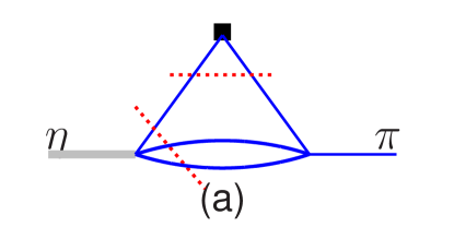
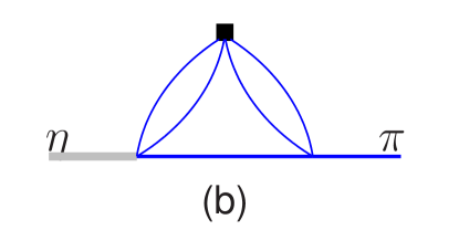
Figure 1: Two types of diagrams contributing to $\eta\pi$ form factors and involving one $\eta\to 3\pi$ vertex.

A usually accepted property of form factors involving two stable particles (like the pion or the nucleon electromagnetic form factors) is that they can be defined as analytic functions of the energy variable $s=(p_{1}-p_{2})^{2}$, with a cut along the positive real axis, the discontinuity along this cut being given by unitarity relations (e.g. [55]).

Here, we wish to consider the $\eta\pi$ form factors $f^{\eta\pi}_{+}$, $f^{\eta\pi}_{0}$ and, since the $\eta$ meson is unstable, one should be concerned about the presence of anomalous thresholds. We illustrate in Fig. 1 the two types of diagrams which involve the $\eta\to 3\pi$ decay amplitude at one vertex. We will consider here contributions of the form of Fig. 1(a) in which the normal threshold is $s_{th}=4m_{\pi}^{2}$. The contributions of the second type, as shown in Fig. 1(b) have a much higher normal threshold $s_{th}=16m_{\pi}^{2}$ and the discontinuity function is expected to be very much suppressed in the region $s\mathrel{\raise 2.32501pt\hbox{$<$}\kern-7.00002pt\lower 2.5187pt\hbox{$\sim$}}1$ $\hbox{GeV}^{2}$ because of the four-body phase space. Let us discuss here the question of the anomalous threshold in the toy model case where Fig. 1(a) represents a Feynman diagram with local vertices. The form factor can then be represented as an integral (e.g. [56])

$$f^{\eta\pi}(s)=\int_{4m_{\pi}^{2}}^{\infty}dt^{\prime}\,\rho(t^{\prime})K^{\eta\pi}(t^{\prime},s)+\cdots$$ (50)

where $K^{\eta\pi}(t^{\prime},s)$ corresponds to the simple triangle Feynman diagram with external momenta $p_{1}^{2}=\bar{m}^{2}_{\eta}$, $p_{2}^{2}=m_{\pi}^{2}$, $p_{3}^{2}=s$ and internal masses $m_{1}^{2}=m_{2}^{2}=m_{\pi}^{2}$, $m_{3}^{2}\equiv t^{\prime}$ (see fig. 2), and the weight function is

$$\rho(t^{\prime})={1\over 16\pi^{2}}\sqrt{1-{4m_{\pi}^{2}\over t^{\prime}}}\ .$$ (51)

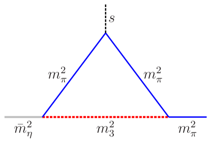
Figure 2: Triangle diagram in eq. (50).

In eq. (50), additional terms (including the UV divergent ones ) have been omitted since they are not concerned with the possibility of an anomalous threshold. We will vary the value of $\bar{m}^{2}_{\eta}$ and, since it can be considered as an energy variable, the amplitude may be defined by appending an infinitesimal positive imaginary part to it, i.e.

$$\bar{m}^{2}_{\eta}\equiv\lim_{\epsilon\to 0}(\bar{m}^{2}_{\eta}+i\epsilon)\ .$$ (52)

We first take $\bar{m}^{2}_{\eta}$ to be sufficiently small (e.g. $\bar{m}^{2}_{\eta}=m_{\pi}^{2}$) such that an ordinary dispersion relation (DR) holds and then increase $\bar{m}^{2}_{\eta}$ until it reaches the physical value $m_{\eta}^{2}$. The ordinary DR for the triangle graph reads,

$$K^{\eta\pi}(t^{\prime},s)={1\over\pi}\int_{4m_{\pi}^{2}}^{\infty}ds^{\prime}\,{L^{\eta\pi}(t^{\prime},s^{\prime})\over s^{\prime}-s}$$ (53)

where $L^{\eta\pi}(t^{\prime},s^{\prime})$ is the discontinuity function of the triangle graph,

$$L^{\eta\pi}(t^{\prime},s^{\prime})={1\over 16\pi\lambda^{1\over 2}(s^{\prime},\bar{m}^{2}_{\eta},m_{\pi}^{2})}\log{a+b\over a-b},$$

$$a=s^{\prime}-(\bar{m}^{2}_{\eta}+3m_{\pi}^{2}-2t^{\prime}),\ b=\sqrt{1-{4m_{\pi}^{2}\over s^{\prime}}}\lambda^{1\over 2}(s^{\prime},\bar{m}^{2}_{\eta},m_{\pi}^{2})\ .$$ (54)

We note that the discontinuity of the form factor is then given as an integral over $L^{\eta\pi}(t^{\prime},s)$

$$\hbox{disc}[f^{\eta\pi}(s)]=\int_{4m_{\pi}^{2}}^{\infty}dt^{\prime}\rho(t^{\prime})L^{\eta\pi}(t^{\prime},s)+\cdots$$ (55)

As discussed in refs. [57, 58] the presence of anomalous thresholds can be inferred from studying the motion of the singularities of the function $L^{\eta\pi}$ upon varying $\bar{m}^{2}_{\eta}$: if one of the singularities crosses the unitarity cut, it is then necessary to deform the contour in the dispersion representation (53), in order to properly define its analytical continuation as a function of $\bar{m}^{2}_{\eta}$, thereby introducing an anomalous threshold. In the present case (4), the singularities of the function $L^{\eta\pi}(t^{\prime},s)$ are given by the solutions of the equation $a^{2}-b^{2}=0$, which is quadratic in $s$

$$t^{\prime}s^{2}+t^{\prime}(t^{\prime}-3m_{\pi}^{2}-\bar{m}^{2}_{\eta}-i\epsilon)s+m_{\pi}^{2}(m_{\pi}^{2}-\bar{m}^{2}_{\eta}-i\epsilon)^{2}=0\ .$$ (56)

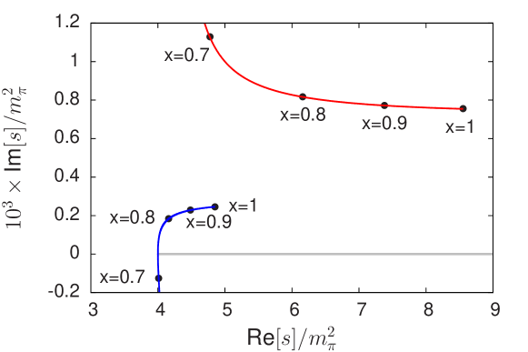
Figure 3: Illustration of the motion of the two singularities of the discontinuity function $L^{\eta\pi}(t^{\prime},s)$ in the $s$ plane for a given value of $t^{\prime}$ when varying the external mass squared $\bar{m}^{2}_{\eta}\equiv xm_{\eta}^{2}$. The plot corresponds to $t^{\prime}=5m_{\pi}^{2}$, $\epsilon=10^{-3}m_{\pi}^{2}$.

Let us consider three cases, depending on the value of the mass variable $t^{\prime}$

1. $t^{\prime}=4m_{\pi}^{2}$: In this case, the two singularities coincide and are given by

   $$s^{\pm}={1\over 2}(\bar{m}_{\eta}^{2}-m_{\pi}^{2}+i\epsilon),$$ (57)

   which is above the unitarity cut.

2. $4m_{\pi}^{2}<t^{\prime}\leq{1\over 2}(\bar{m}_{\eta}^{2}-m_{\pi}^{2})$: This is the most interesting situation, the motion of the two singularities $s^{\pm}(\bar{m}^{2}_{\eta})$ as a function of $x=\bar{m}^{2}_{\eta}/m_{\eta}^{2}$ is illustrated in Fig. 3. The figure shows that while $s^{+}(\bar{m}^{2}_{\eta})$ remains above the real axis, the other singularity does cross the real axis very close to $4m_{\pi}^{2}$. It is easy to see that the crossing occurs when $\bar{m}^{2}_{\eta}=m_{\pi}^{2}+2t^{\prime}$ and the value of the crossing point is

   $$s^{-}(m_{\pi}^{2}+2t^{\prime})=4m_{\pi}^{2}\left(1-{\epsilon^{2}\over 4t^{\prime}(t^{\prime}-4m_{\pi}^{2})}\right)\ ,$$ (58)

   which is located strictly below the normal threshold.

3. ${1\over 2}(\bar{m}_{\eta}^{2}-m_{\pi}^{2})<t^{\prime}\leq(\bar{m}_{\eta}-m_{\pi})^{2}$: In this case $s^{+}(\bar{m}_{\eta}^{2})$ remains above the real axis and $s^{-}(\bar{m}^{2}_{\eta})$ remains below it.

For larger values of $t^{\prime}$, it is easily verified that $s^{\pm}(\bar{m}_{\eta}^{2})$ do not come close to the unitarity cut. The conclusion of this discussion is that, for a Feynman diagram, the amplitude as given from Fig. 1(a) does not involve any anomalous threshold. We will argue in the next section that the same conclusion holds in a more realistic approach where the $\eta\to 3\pi$ amplitude is given from Khuri-Treiman equations solutions. The fact that the $\eta$ meson is unstable, i.e. $m_{\eta}>3m_{\pi}$, manifests itself in the violation of real analyticity, the discontinuity function is complex and does not coincide with the imaginary part of the diagram (the latter, indeed, is given by the sum of two Cutkosky contributions, corresponding to two physically allowed ways of cutting the diagram; see Fig. 1(a)).

5 Dispersive evaluation of $f^{\eta\pi}_{+}$

We have argued in sec. 2 that the dominant contribution to the discontinuity of $f^{\eta\pi}_{+}(s)$, with $s\mathrel{\raise 2.32501pt\hbox{$<$}\kern-7.00002pt\lower 2.5187pt\hbox{$\sim$}}1$ $\hbox{GeV}^{2}\$, was from the $n=\pi^{0}\pi^{+}$ state. Then, $\hbox{disc}[f^{\eta\pi}_{+}]$ was found to be proportional to the pion vector form factor $F_{V}^{\pi}$, which is well known from experiment, and to the $l=1$ projection of the $\eta\pi^{+}\to\pi^{0}\pi^{+}$ amplitude. In order to evaluate this amplitude, we will make use of the work of refs. [18, 19], who developed and solved a set of Khuri-Treiman [16] equations and applied the results in the physical region of the $\eta\to 3\pi$ decay. We briefly recall the main features of this formalism below (a very detailed account can be found in the thesis [59]). As it encodes the analyticity properties of the $\eta\pi^{+}\to\pi^{0}\pi^{+}$ amplitude, this formalism should be suitable for evaluating the amplitude in the partly unphysical region needed for computing $\hbox{disc}[f^{\eta\pi}_{+}]$.

5.1 Brief review of the Khuri-Treiman formalism

The Khuri-Treiman (KT) equations implement dispersion relations, crossing symmetry and unitarity in the approximation where a single state, $n=\pi\pi$, is retained in the unitarity relations. This approximation is acceptable when the Mandelstam variables $s$, $t$, $u$ are smaller than 1 ${\rm GeV}^{2}$ in magnitude. It was noted in refs. [18, 19] that, in the same region, the contributions from the discontinuities of the partial-waves $J\geq 2$ can also be neglected in the dispersion relations such that the decomposition theorem [60] may be applied to the $\eta\to 3\pi$ amplitude. As a result, it can be expressed in terms of three functions of a single variable, $M_{I}(w)$,

$$T_{\eta\pi^{0}\to\pi^{-}\pi^{+}}(s,t,u)=T_{\eta\pi^{+}\to\pi^{0}\pi^{+}}(t,s,u)=-\epsilon_{L}\times\!\Big{[}M_{0}(s)+(s-u)M_{1}(t)$$

$$\phantom{T_{\eta\pi^{0}\to\pi^{-}\pi^{+}}(s,t,u)=}+(s-t)M_{1}(u)+M_{2}(t)+M_{2}(u)-{2\over 3}M_{2}(s)\Big{]}$$ (59)

with

$$\epsilon_{L}={1\over Q^{2}}{m_{K}^{2}\over m_{\pi}^{2}}\,{m_{K}^{2}-m_{\pi}^{2}\over 3\sqrt{3}F_{\pi}^{2}},\quad Q^{2}={m_{s}^{2}-\hat{m}^{2}\over m_{d}^{2}-m_{u}^{2}}\ .$$ (60)

Based on usual Regge phenomenology for estimating the asymptotic behaviour, it was concluded in ref. [19] that $M_{0}$, $M_{2}$ should obey converging DR’s with two subtractions and $M_{1}$ a converging DR with a single subtraction,

$$M_{0}(w)=\tilde{\alpha}_{0}+\tilde{\beta}_{0}w+{w^{2}\over\pi}\int_{4m_{\pi}^{2}}^{\infty}ds^{\prime}\,\frac{\hbox{disc}[M_{0}(s^{\prime})]}{(s^{\prime})^{2}(s^{\prime}-w)}$$

$$M_{1}(w)={w\over\pi}\int_{4m_{\pi}^{2}}^{\infty}ds^{\prime}\,\frac{\hbox{disc}[M_{1}(s^{\prime})]}{s^{\prime}(s^{\prime}-w)}$$

$$M_{2}(w)={w^{2}\over\pi}\int_{4m_{\pi}^{2}}^{\infty}ds^{\prime}\,\frac{\hbox{disc}[M_{2}(s^{\prime})]}{(s^{\prime})^{2}(s^{\prime}-w)}\ .$$ (61)

In writing these DR’s one has further made use of freedom to redefine $M_{I}$ by linear functions without modifying the $\eta\pi\to\pi\pi$ amplitude in eq. (5.1) because of the constraint $s+t+u=m_{\eta}^{2}+3m_{\pi}^{2}\equiv 3s_{0}$. The functions $M_{I}(w)$ are analytic in the complex $w$ plane except for a cut along the real axis along $[4m_{\pi}^{2},\infty]$. The discontinuity along this cut is obtained from the unitarity relations of the $J=0,1$ partial-wave projections of the $\eta\pi\to\pi\pi$ amplitudes and they read,

$$\hbox{disc}[M_{I}(s)]_{\pi\pi}=\theta(s-4m_{\pi}^{2})\,e^{-i\delta_{I}(s)}\sin\delta_{I}(s)(M_{I}(s+i\epsilon)+\hat{M}_{I}(s))\ .$$ (62)

In eq. (62) the functions $\hat{M}_{I}$ are linear combinations of the angular integrals,

$${\langle z^{n}M_{I}\rangle}(s)={1\over 2}\int_{-1}^{1}dzz^{n}M_{I}(t(s,z))$$ (63)

with

$$t(s,z)={1\over 2}(3s_{0}-s+\kappa(s)z),\ \kappa(s)=\sqrt{1-4m_{\pi}^{2}/s}\sqrt{\lambda_{\eta\pi}{(s)}}\ .$$ (64)

The explicit expressions of $\hat{M_{I}}$ in terms of the angular integrals read [19]

$$\hat{M}_{0}={2\over 3}{\langle M_{0}\rangle}+{20\over 9}{\langle M_{2}\rangle}+2(s-s_{0}){\langle M_{1}\rangle}+{2\over 3}\kappa{\langle zM_{1}\rangle}$$

$$\hat{M}_{1}=\kappa^{-1}\left\{3{\langle zM_{0}\rangle}-5{\langle zM_{2}\rangle}+{9\over 2}(s-s_{0}){\langle zM_{1}\rangle}+{3\over 2}\kappa{\langle z^{2}M_{1}\rangle}\right\}$$

$$\hat{M}_{2}={\langle M_{0}\rangle}+{1\over 3}{\langle M_{2}\rangle}-{3\over 2}(s-s_{0}){\langle M_{1}\rangle}-{1\over 2}\kappa{\langle zM_{1}\rangle}\ .$$ (65)

Eqs. (5.1) and (62) (5.1) are a first form of the Khuri-Treiman integral equations for the $\eta\pi\to\pi\pi$ amplitude.

5.2 Singularities of the functions $\hat{M}_{I}$

Using the representation of $T_{\eta\pi\to\pi\pi}$ based on the decomposition theorem (5.1), we can now write the discontinuity of the form factor $f^{\eta\pi}_{+}$ as

$$\hbox{disc}[f^{\eta\pi}_{+}(s)]_{\pi\pi}=\theta(s-4m_{\pi}^{2}){(s-4m_{\pi}^{2})^{3\over 2}\over 48\pi\sqrt{s}}\epsilon_{L}F_{V}^{\pi}(s-i\epsilon)(M_{1}(s+i\epsilon)+\hat{M}_{1}(s))\ .$$ (66)

For completeness, let us mention the analogous relation for the scalar form factor,

$$\hbox{disc}[f^{\eta\pi}_{0}]_{\pi\pi}=\theta(s-4m_{\pi}^{2}){(s-4m_{\pi}^{2})^{1\over 2}\over 16\pi\sqrt{s}}{\Delta_{{\pi^{0}}{\pi^{+}}}\over\Delta_{\eta{\pi^{+}}}}\epsilon_{L}f_{0}^{\pi\pi}(s-i\epsilon)(M_{2}(s+i\epsilon)+\hat{M}_{2}(s))\ .$$ (67)

Adapting the discussion of sec. 4 about the presence of anomalous thresholds to the present, more realistic situation, requires one to investigate the singularities of the functions $\hat{M}_{I}(w)$ i.e. of the angular integrals given in (63). This can be done by inserting the dispersive representations of the functions $M_{I}$ (eqs. (5.1)) into the angular integrals (eqs. (63)) from which one obtains an expression of the functions ${\langle z^{n}M_{I}\rangle}$ as integrals over kernels $K^{(n)}(t^{\prime},w)$, $P^{(n)}(t^{\prime},w)$

$${\langle M_{0}\rangle}(w)=\tilde{\alpha}_{0}+{1\over 2}(3s_{0}-s)\tilde{\beta}_{0}-{1\over\pi}\int_{4m_{\pi}^{2}}^{\infty}dt^{\prime}K^{(0)}(t^{\prime},w)\,\hbox{disc}[M_{0}(t^{\prime})]$$

$${\langle zM_{0}\rangle}(w)={1\over 6}\kappa(w)\tilde{\beta}_{0}-{1\over\pi}\int_{4m_{\pi}^{2}}^{\infty}dt^{\prime}K^{(1)}(t^{\prime},w)\,\hbox{disc}[M_{0}(t^{\prime})]$$

$${\langle z^{n}M_{2}\rangle}(w)=-{1\over\pi}\int_{4m_{\pi}^{2}}^{\infty}dt^{\prime}K^{(n)}(t^{\prime},w)\,\hbox{disc}[M_{2}(t^{\prime})]$$

$${\langle z^{n}M_{1}\rangle}(w)=-{1\over\pi}\int_{4m_{\pi}^{2}}^{\infty}dt^{\prime}P^{(n)}(t^{\prime},w)\,\hbox{disc}[M_{1}(t^{\prime})]\ .$$ (68)

The kernels which are needed here are given explicitly in appendix A. They involve the logarithmic function

$$L(t^{\prime},w)={1\over 2}\int_{-1}^{1}dz\,{1\over t(w,z)-t^{\prime}}\ .$$ (69)

which controls their singularity structure. When performing the angular integration in eqs. (63), (69) one must keep in mind that the path of integration from $z=-1$ to $z=1$ must eventually be deformed in order not to intersect with the cut of the functions $M_{I}$, i.e. $4m_{\pi}^{2}\leq t(w,z)<\infty$, as is explained in detail in ref. [18]. The following expression of the logarithmic function exactly encodes these prescriptions on the integration path in a simple way,

$$L(t^{\prime},w)={\log(t^{\prime}-t^{+}(w))-\log(t^{\prime}-t^{-}(w))\over t^{+}(w)-t^{-}(w)}$$ (70)

where

$$t^{\pm}(w)={1\over 2}\Big{(}m_{\eta}^{2}+i\epsilon+3m_{\pi}^{2}-w\pm\sqrt{1-{4m_{\pi}^{2}\over s}}\lambda^{1\over 2}(m_{\eta}^{2}+i\epsilon,m_{\pi}^{2},w)\Big{)}$$ (71)

displaying explicitly the $i\epsilon$ prescription. From the form of the logarithmic function (70), (71) we can infer the following consequences:

1. Absence of anomalous thresholds: Inserting the representation of $\hat{M}_{1}$, $\hat{M}_{0}$ in terms of the kernels (5.2) one obtains an integral representation of the form factor discontinuities $\hbox{disc}[f^{\eta\pi}_{+}]$, $\hbox{disc}[f^{\eta\pi}_{0}]$ in terms of the logarithm function (70) which is analogous to eq. (55). Furthermore, the singularities of the logarithms are exactly the same. Therefore, the conclusion about the absence of anomalous thresholds, as discussed in sec. 4, applies also in the present realistic situation.

2. Cuts ${\cal C}$ of the $\hat{M}_{I}$ functions: They are given, using the integral representations in terms of kernels, as the ensemble of the singularities of the logarithmic function (70) (see [61]) i.e. the points $w$ which satisfy $t^{\pm}(w)=t^{\prime}$. This relation can be recast as a quadratic equation in $w$ identical to (56). Therefore,

   $${\cal C}=\{w:w=t^{\pm}(t^{\prime}),\ 4m_{\pi}^{2}\leq t^{\prime}<\infty\},$$ (72)

   The curve (72) includes the negative real axis, it extends into the complex plane and approaches infinitesimally close to the unitarity cut on the positive real axis in the region $4m_{\pi}^{2}\leq w\leq(m_{\eta}-m_{\pi})^{2}$ without, however, crossing it: this is shown on fig. 4. As a consequence, the functions $\hat{M}_{I}(s^{\prime})$ are unambiguously defined on the real axis in the integration range $4m_{\pi}^{2}\leq s^{\prime}<\infty$.

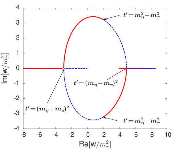
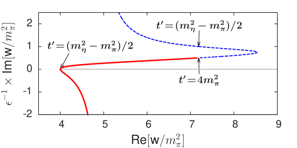
Figure 4: Complex cut ${\cal C}$ of the functions $\hat{M}_{I}(w)$ (see eq. (72): the solid (dashed) curves correspond to the points which satisfy $w=t^{-}(t^{\prime})$ ($t^{+}(t^{\prime})$). The lower figure shows an enlarged view of the vicinity of the unitarity cut.

The point $w=m_{-}^{2}\equiv(m_{\eta}-m_{\pi})^{2}$ requires special attention. At this point the difference between $t^{+}(w)$ and $t^{-}(w)$ is infinitesimal but their imaginary parts have different signs

$$t^{\pm}(m_{-}^{2})=m_{\pi}(m_{\eta}+m_{\pi})\pm{i\sqrt{\epsilon}\over 2}\sqrt{m_{\pi}(m_{\eta}-m_{\pi})}$$ (73)

which implies that the logarithmic function $L(t^{\prime},w)$ diverges when $\epsilon$ goes to zero and $t^{\prime}$ lies in the range $4m_{\pi}^{2}\leq t^{\prime}<m_{\pi}(m_{\eta}+m_{\pi})$

$$\lim_{w\to m_{-}^{2}}L(t^{\prime},w)={2\pi\over\sqrt{\epsilon}}{\theta(m_{\pi}(m_{\eta}+m_{\pi})-t^{\prime})\over\sqrt{m_{\pi}(m_{\eta}-m_{\pi})}}$$ (74)

which induces a divergence in the functions $\hat{M_{I}}(w)$ when $w\to m_{-}^{2}$

$$\lim_{w\to m_{-}^{2}}\hat{M}_{0}(w),\,\hat{M}_{2}(w)\sim O(\epsilon^{-{1\over 2}}),\quad\lim_{w\to m_{-}^{2}}\hat{M}_{1}(w)\sim O(\epsilon^{-{3\over 2}})\ .$$ (75)

However, integrals over $\hat{M}_{I}$ (as in eqs. (5.2), (78)) remain finite in the $\epsilon\to 0$ limit [18] such that the functions $M_{I}(w)$ themselves do no exhibit any divergence. The numerical treatment of the integrations involving $\hat{M}_{I}$ is the delicate part of solving the KT equations. When the integration variable is close to $m_{-}^{2}$ one must perform expansions in powers of $\sqrt{m_{-}^{2}-t^{\prime}}$ and use the analytical expressions for the integrals of the functions $\log(t^{\prime}-t^{\pm}(w))/(m_{-}^{2}-t^{\prime}+i\epsilon)^{n+1/2}$ (appearing in eq. (5.2)) and $1/((t^{\prime}-w-i\epsilon)(m_{-}^{2}-t^{\prime}+i\epsilon)^{n+1/2})$ (in eq. (78)). Analogous singular integrations appear in the dispersive representation of the vector form factor $f^{\eta\pi}_{+}$ as its discontinuity involves $\hat{M}_{1}$.

5.3 Matching with ChPT

In the form given by eqs. (5.1) (62) (5.1) the KT equations are linear integral equations with a singular Cauchy kernel. The most general solutions of such integral equations involve an arbitrary number of polynomial parameters [62, 63]. Physically, the polynomial growth is limited by asymptotic conditions on the amplitudes. In practice, however, the system of equations is valid only in the elastic scattering region, while the integrals run up to infinity. The polynomial part must thus be considered as a parametrisation of the corrections to the effects of the integration regions $s^{\prime},t^{\prime}\geq 1$ $\hbox{GeV}^{2}\$over the solutions in the elastic scattering region. For our purposes, we will consider here a four-parameter family of solutions. The polynomial dependence is exhibited by introducing the Omnès functions,

$$\Omega_{I}(w)=\exp\left[{w\over\pi}\int_{4m_{\pi}^{2}}^{\infty}ds^{\prime}\,{\delta_{I}(s^{\prime})\over s^{\prime}(s^{\prime}-w)}\right]$$ (76)

where $\delta_{I}$ is equal to the $S$ or $P$-wave $\pi\pi$ phase shift with isospin $I$ in the elastic region. The functions $M_{I}$ are then expressed as

$$M_{0}(w)=\Omega_{0}(w)\left(\alpha_{0}+\beta_{0}w+\gamma_{0}w^{2}+w^{2}\hat{I}_{0}(w)\right)$$

$$M_{1}(w)=\Omega_{1}(w)\left(\beta_{1}w+w\hat{I}_{1}(w)\right)$$

$$M_{2}(w)=\Omega_{2}(w)\left(w^{2}\hat{I}_{2}(w)\right)$$ (77)

where

$$\hat{I}_{a}(w)={1\over\pi}\int_{4m_{\pi}^{2}}^{\infty}ds^{\prime}{\sin\delta_{a}(s^{\prime})\hat{M}_{a}(s^{\prime})\over(s^{\prime})^{2-n_{a}}(s^{\prime}-w)|\Omega_{a}(s^{\prime})|},\quad n_{a}=\delta_{1a},$$ (78)

which ensure that the discontinuity eqs. (62) are obeyed. The two subtraction constants which appear in the dispersive representation (5.1) are simply related to the polynomial parameters: $\tilde{\alpha}_{0}=\alpha_{0}$, $\tilde{\beta}_{0}=\beta_{0}+\alpha_{0}\dot{\Omega}(0)$. Plugging this representation into eq. (5.1) one obtains a set of linear integral equations for the functions $\hat{M}_{I}$. As these are not singular equations anymore, one may thus expect that, for given values of the parameters $\alpha_{0}$, $\beta_{0}$, $\gamma_{0}$, $\beta_{1}$, if a solution exists for $\hat{M}_{I}$, it should be unique[19].

The most natural idea for determining the polynomial parameters is by matching the KT amplitude with the amplitude computed in the chiral expansion [17, 18, 19] in the region where the variables $s$, $t$, $u$ are small. More precisely, if $\macc@depth\char 1\relax\frozen@everymath{\macc@group}\macc@set@skewchar\macc@nested@a 111{M}(s,t,u)$ is the amplitude computed to chiral order $p^{N}$, then the parameters $\alpha_{0}$, $\beta_{0}$, $\beta_{1}$, $\gamma_{0}$ should be such that

$$M(s,t,u)-\macc@depth\char 1\relax\frozen@everymath{\macc@group}\macc@set@skewchar\macc@nested@a 111{M}(s,t,u)=O(p^{N+2})\ .$$ (79)

Considering the $N=4$ case, a first observation is that the differences of the discontinuities in each of the component functions $M_{I}$ are of chiral order $p^{6}$,

$$\hbox{disc}[M_{I}(w)-\macc@depth\char 1\relax\frozen@everymath{\macc@group}\macc@set@skewchar\macc@nested@a 111{M}_{I}(w)]=O(p^{6})$$ (80)

independently of the values of the polynomial parameters. This implies that the $O(p^{4})$ parts of the differences $M_{I}(w)-\macc@depth\char 1\relax\frozen@everymath{\macc@group}\macc@set@skewchar\macc@nested@a 111{M}_{I}(w)$ must be polynomial. Imposing that the $O(p^{4})$ parts of polynomial expansions of the differences $M_{I}-\macc@depth\char 1\relax\frozen@everymath{\macc@group}\macc@set@skewchar\macc@nested@a 111{M}_{I}$ vanish yields the following four matching equations [19]

$$\begin{array}[]{ll}\alpha_{0}=&9\,\big{(}\dfrac{1}{2}\macc@depth\char 1\relax\frozen@everymath{\macc@group}\macc@set@skewchar\macc@nested@a 111{M}^{\prime\prime}_{2}-\hat{I}_{2}\big{)}\,s_{0}^{2}+3(\macc@depth\char 1\relax\frozen@everymath{\macc@group}\macc@set@skewchar\macc@nested@a 111{M}^{\prime}_{2}-\macc@depth\char 1\relax\frozen@everymath{\macc@group}\macc@set@skewchar\macc@nested@a 111{M}_{1})\,s_{0}+\macc@depth\char 1\relax\frozen@everymath{\macc@group}\macc@set@skewchar\macc@nested@a 111{M}_{0}+\dfrac{4}{3}\macc@depth\char 1\relax\frozen@everymath{\macc@group}\macc@set@skewchar\macc@nested@a 111{M}_{2}\\[7.11317pt] \beta_{0}=&\!\!\!-9\,\big{(}\dfrac{1}{2}\macc@depth\char 1\relax\frozen@everymath{\macc@group}\macc@set@skewchar\macc@nested@a 111{M}^{\prime\prime}_{2}-\hat{I}_{2}\big{)}\,s_{0}+\macc@depth\char 1\relax\frozen@everymath{\macc@group}\macc@set@skewchar\macc@nested@a 111{M}^{\prime}_{0}+3\macc@depth\char 1\relax\frozen@everymath{\macc@group}\macc@set@skewchar\macc@nested@a 111{M}_{1}-\dfrac{5}{3}\macc@depth\char 1\relax\frozen@everymath{\macc@group}\macc@set@skewchar\macc@nested@a 111{M}^{\prime}_{2}-\Omega^{\prime}_{0}\alpha_{0}\\[7.11317pt] \beta_{1}=&\macc@depth\char 1\relax\frozen@everymath{\macc@group}\macc@set@skewchar\macc@nested@a 111{M}^{\prime}_{1}+\dfrac{1}{2}\macc@depth\char 1\relax\frozen@everymath{\macc@group}\macc@set@skewchar\macc@nested@a 111{M}^{\prime\prime}_{2}-\hat{I}_{1}-\hat{I}_{2}\\[7.11317pt] \gamma_{0}=&\dfrac{1}{2}\macc@depth\char 1\relax\frozen@everymath{\macc@group}\macc@set@skewchar\macc@nested@a 111{M}^{\prime\prime}_{0}+\dfrac{2}{3}\macc@depth\char 1\relax\frozen@everymath{\macc@group}\macc@set@skewchar\macc@nested@a 111{M}^{\prime\prime}_{2}-\hat{I}_{0}-\dfrac{4}{3}\hat{I}_{2}-\dfrac{1}{2}\Omega^{\prime\prime}_{0}\alpha_{0}-\Omega^{\prime}_{0}\beta_{0}\ .\end{array}$$ (81)

where the functions $\macc@depth\char 1\relax\frozen@everymath{\macc@group}\macc@set@skewchar\macc@nested@a 111{M}_{a}$, $\Omega_{a}$, $\hat{I}_{a}$ and their derivatives are all to be taken at $w=0$. In order to solve the set of eqs. (81), one must keep in mind that the integrals $\hat{I}_{a}$ carry an implicit linear dependence on the four polynomial parameters. This dependence must be determined by using four independent KT solutions in which one of the polynomial parameters is set to one and the others to zero.

The chiral NLO amplitude $\macc@depth\char 1\relax\frozen@everymath{\macc@group}\macc@set@skewchar\macc@nested@a 111{M}(s,t,u)$ was first computed in ref. [11], it is given in ref. [19] in a form which involves a single $O(p^{4})$ coupling constant, $L_{3}$. We will use here the value $L_{3}=(-3.04\pm 0.43)10^{-3}$ [64].

5.4 Numerical solutions and comparisons with the $\eta\to 3\pi$ data

We have constructed numerical solutions of the set of KT equations by iteration. The main differences with earlier work[18, 19] is that:

• we have used the kernel representations (5.2) for performing the angular integrations, which should be somewhat faster than the integration over a complex contour method used previously,

• The matching with ChPT was done via the four matching equations (81), which were solved with no approximations.

In ref. [19] only the last two matching equations were implemented while the first two were replaced by imposing that the amplitude $M(s,t,u)$ along the line $u=s$ has an Adler zero at the same position and with the same slope as the chiral NLO amplitude. We will see below (fig. 6 ) that the first two matching relations ensure essentially equivalent constraints on the Adler zero.

Concerning the phases $\delta_{I}(s)$ for $I=1$ and $I=2$, for which inelasticity sets in rather smoothly, we take the phases to be equal to the corresponding $\pi\pi$ scattering phase shifts up to $\sqrt{s}_{cut}=1.4$ GeV and, for $s>s_{cut}$ interpolate to the asymptotic values $\delta_{1}(\infty)=\pi$ and $\delta_{2}(\infty)=0$.

	$\alpha_{0}$	$\beta_{0}$	$\beta_{1}$	$\gamma_{0}$
cutoff(1)	$-0.60+i0.07$	$15.7-i0.69$	$6.95+i0.40$	$-0.77+i0.86$
cutoff(2)	$-0.61+i0.08$	$16.5-i0.88$	$6.89+i0.47$	$-26.5+i1.76$
fit	$-0.77-i0.02$	$19.8-i0.17$	$4.75$	$-34.9$

Table 1: Influence of the cutoff conditions (see text) for the phase $\delta_{0}$ on the values of the polynomial parameters derived from the matching equations (in appropriate powers of GeV). Also shown are the results of fitting two parameters to the experimental Dalitz plot results.

In the case of the $I=0$ $S$-wave, inelasticity sets in sharply around the $K\bar{K}$ threshold. We have employed two different phase choices in the inelastic region: a) the one used in ref. [18] (which we call cutoff (1)): for $s$ larger than $s_{cut}=(0.865)^{2}$ GeV², the phase is interpolated rapidly to $\delta_{0}(\infty)=0$ and b) a condition similar to that used in ref. [59]) (which we call cutoff (2)): for $s$ larger than $4m_{K}^{2}$, the phase is interpolated slowly to $\delta_{0}(\infty)=\pi$. These phases are illustrated in fig. 5. When used in the matching relations (81) these different conditions lead to rather different values for some of the polynomial parameters,, reflecting differences in the values of the integral $\hat{I}_{0}(0)$ as well as in the values of the Omnès function and its derivatives at $s=0$ (see table 1). However, the matching conditions ensure that the complete KT amplitude depends only moderately on the cutoff conditions. Fig. 6 illustrates some results, showing amplitudes along the line $t=s$ where an Adler zero is present in the chiral amplitude.

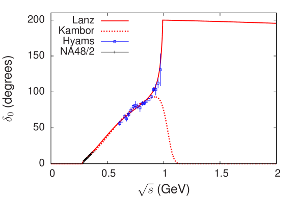
Figure 5: Illustration of $I=0$ phases used for computing the Omnès function $\Omega_{0}$ (eq. (76)) based on different assumptions in the inelastic region. The solid line is analogous to the phase used in ref. [59] and the dashed line is the phase used in ref. [18]. Also shown are some experimental $\pi\pi$ data from refs. [65, 66].

In order to assess the reliability of the $\eta\pi\to\pi\pi$ amplitude resulting from KT solutions with ChPT matching, let us compare with experimental results. From the integrated decay rate of the charged mode: $\Gamma_{\eta\to\pi^{0}\pi^{-}\pi^{+}}^{exp}=300\pm 11$ eV [67], one obtains for the central value of the double quark mass ratio: $Q\simeq 21.6$ with the cutoff (1) condition and $Q\simeq 21.5$ with the cutoff (2). This value is compatible with the result of ref. [18] ($Q=21.6\pm 1.3$, with NLO matching) and slightly smaller than the one quoted in ref. [59] ($Q=22.7$), based on the same formalism, but a somewhat different implementation of the matching with ChPT. The corresponding value of the quark mass ratio $\epsilon$, is $\epsilon=1.32\cdot 10^{-2}$. Using this value of $\epsilon$ in the chiral expansion of $f^{\eta\pi}_{+}(0)$, eq. (3.1), on obtains a result compatible with the one given in eq. (40), derived from experimental data of $K^{+}_{l3}$, $K^{0}_{l3}$ decays.

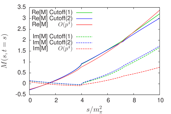
Figure 6: Results for the amplitude $M(s,t)$ along the line $t=s$ obtained from solving the KT equations together with the four chiral matching relations (81) using two different cutoff conditions for the phase $\delta_{0}$. Also shown is the chiral $O(p^{4})$ amplitude.

Precise measurements of the differential decay distributions across the Dalitz plot have been performed recently for both the charged [10] and the neutral decay modes [6, 7, 8, 9]. It is customary to represent these differential distributions in terms of a polynomial of two independent energy variables $X$, $Y$ (defined such that $X^{2}+Y^{2}\leq 1$ and $X=Y=0$ corresponds to the center of the Dalitz plot, where the three pions have equal kinetic energies, see appendix C)

$${d^{2}\Gamma_{c}\over dXdY}(X,Y)={d^{2}\Gamma_{c}\over dXdY}(0,0)\left(1+aY+bY^{2}+dX^{2}+fY^{3}+\cdots\right)$$ (82)

for the charged mode, and

$${d^{2}\Gamma_{n}\over dXdY}(X,Y)={d^{2}\Gamma_{n}\over dXdY}(0,0)\left(1+\alpha(X^{2}+Y^{2})+\cdots\right)$$ (83)

for the neutral mode. The experimental values of the Dalitz plot parameters $a$, $b$, $d$, $f$ and $\alpha$ are shown in table 2 together with results corresponding to KT solutions amplitudes. Implementation of rescattering effects via the KT equations leads to significantly improved results with respect to the simple use of the chiral NLO amplitude (see [11]) but the two Dalitz parameters $b$ and $d$ are still predicted to be too large.

Dalitz par.	experimental	cutoff(1)	cutoff(2)	Fit
a	$-1.090\pm 0.005^{+0.008}_{-0.019}$	$-1.171$	$-1.125$	$-1.062$
b	$0.124\pm 0.006\pm 0.010$	$0.260$	$0.196$	$0.163$
d	$0.057\pm 0.006^{+0.007}_{-0.016}$	$0.083$	$0.082$	$0.067$
f	$0.14\pm 0.01\pm 0.02$	$0.074$	$0.100$	$0.102$
$\alpha$	$-0.0315\pm 0.0015$	$-0.0127$	$-0.0260$	$-0.0336$

Table 2: Comparison between the experimental values of the Dalitz plot parameters for $\eta\to\pi^{0}\pi^{+}\pi^{-}$ and $\eta\to 3\pi^{0}$ and the predictions of the KT solution amplitudes with NLO matching and two different cutoff conditions (see table 1). The last column shows the result of a KT solution where part of the polynomial parameters are fitted to the data.

This discrepancy between the theoretical amplitude and experiment indicates that further effects need to be taken into account. These could be either chiral $O(p^{6})$ effects at the level of the matching equations or further rescattering effects. In this respect, one sees clearly from table 2 that the $\pi\pi$ phase choice which does include the $f_{0}(980)$ resonance leads to better results for the Dalitz plot parameters than the choice which does not. It is then not unlikely that the $a_{0}(980)$ resonance should be taken into account as well. It is also worth noting that preliminary results from analysis of new data sets by KLOE and WASA have been presented (see [68], p.16) which go in the direction of improving the agreement with the theoretical predictions.

For our present purposes, in addition to the KT amplitudes which obey the ChPT matching relations, we construct an amplitude which reproduces more closely the experimental results on the Dalitz plot. In order to do so, we allow the two polynomial parameters $\beta_{1}$, $\gamma_{0}$ to vary freely (still assuming their imaginary parts to be negligible) and use them as fit parameters. The last two polynomial parameters $\alpha_{0}$, $\beta_{0}$ are then fixed from the two conditions: 1) that the amplitude reproduces the position of the Adler zero $s_{A}$ of the NLO amplitude and 2) that the central value of the quark mass double ratio $Q$ from lattice QCD (the recent FLAG review [50] gives $Q^{latt}=22.6(7)(6)$ from $N_{f}=2+1$ simulations) is reproduced. The results from this amplitude for Dalitz plot parameters are displayed in the last column of table 2 and the corresponding polynomial parameters are shown on the last line of table 1.

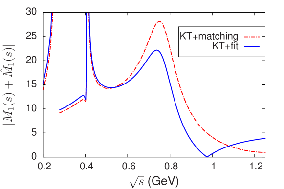
Figure 7: Modulus of function $M_{1}+\hat{M}_{1}$ obtained from KT solutions with two sets of polynomial parameters. Dash-dotted curve: parameters from $O(p^{4})$ matching (cutoff (2)), solid curve: parameters from fit.

5.5 Results for $f^{\eta\pi}_{+}$

In the elastic scattering region, the discontinuity of $f^{\eta\pi}_{+}(s)$ was given in eq. (a)) in terms of the pion form factor $F_{V}^{\pi}$ and the $l=1$ projection of the $\eta\pi^{+}\to\pi^{0}\pi^{+}$ amplitude. From the decomposition theorem, this projected amplitude may be expressed in terms of $M_{1}+\hat{M}_{1}$ (eq. (66)). We can now calculate this quantity from our solutions of the KT equations. Fig. 7 shows the numerical results for the modulus of $M_{1}+\hat{M}_{1}$. It illustrates the strong sensitivity to the choice of the polynomial parameters. The solution corresponding to fitted parameters (last line in table 1) has a significantly smaller resonance peak, which is related to the smaller size of the parameter $\beta_{1}$.

Concerning the pion form factor, we used the experimental measurements of $|F_{V}^{\pi}|$ from $\tau$ decays (which provide exactly the same form factor as needed here) by the Belle collaboration [69]. The measurement covers the energy range $0.297\leq\sqrt{s}\leq 1.255$ GeV which is essentially adequate for our purposes. We relied on the fit performed in ref. [69] in terms of Gounaris-Sakurai (GS) functions [70] for performing an extrapolation of $|F_{V}^{\pi}|$ in the small energy region down to the threshold and performing the numerical integrations. For the phase $\delta_{V}^{\pi}$, we assumed elastic unitarity to hold below 1 GeV and thus took $\delta_{V}^{\pi}$ to be equal to the $l=1$ $\pi\pi$ phase shift in accordance with Watson’s theorem. Above 1 GeV, we use the phase as predicted by the GS parametrisation.

Asymptotically, from the usual QCD-based arguments [71, 72], one expects the form factor $f^{\eta\pi}_{+}(s)$ to behave as $1/s\log(s)$, it should thus obey a convergent dispersion relation. We will actually use DR’s for $f^{\eta\pi}_{+}(s)/s^{N}$ in order to suppress the contribution from the integration region above 1 GeV. In practice, we will use $N=1$ or $N=2$ and check the stability of the result. For example, with $N=2$, the DR reads

$$f^{\eta\pi}_{+}(s)=f^{\eta\pi}_{+}(0)+s\dot{f}^{\eta\pi}_{+}(0)+{s^{2}\over\pi}\int_{4m_{\pi}^{2}}^{\infty}ds^{\prime}\,{\hbox{disc}[f^{\eta\pi}_{+}(s^{\prime})]\over(s^{\prime})^{2}(s^{\prime}-s)}\ .$$ (84)

The values of $f^{\eta\pi}_{+}$ and its derivative at $s=0$ from NLO ChPT were given in sec. 3. The value of the quark mass ratio $\epsilon$ used in eq. (43) was deduced from the quark mass double ratio $Q$ corresponding to the KT amplitude used (i.e. either $Q=21.5$ with matched polynomial parameters or $Q=22.6$ with fitted parameters) and using the central value of the result given in the FLAG review [50]: $2m_{s}/(m_{u}+m_{d})=27.46(15)(41)$.

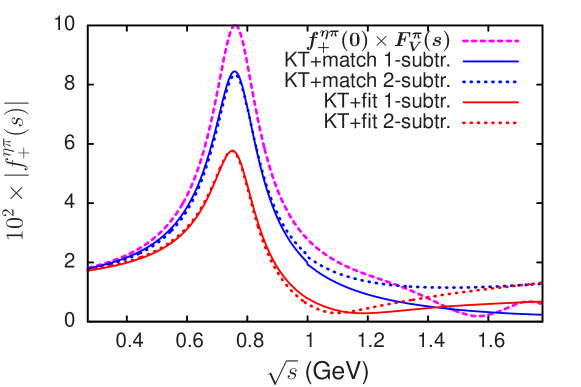
Figure 8: Dispersive calculations of the vector form factor $f^{\eta\pi}_{+}$. The upper and lower solid lines correspond to once-subtracted dispersion dispersion relations using KT amplitudes with matched and with fitted parameters respectively. The dotted lines correspond to twice subtracted dispersion relations. The pion vector form factor normalised to $f^{\eta\pi}_{+}(0)$ at $s=0$ is also shown for comparison (dashed line).

The results obtained using these dispersion relations together with $\eta\pi\to\pi\pi$ amplitudes from KT equations and also using the parametrisation given by the Belle collaboration [69] for the pion form factor are shown in fig. 8. The figure shows that the DR’s with $N=1$ or $N=2$ yield very similar results in the region $\sqrt{s}\leq 1$ GeV. As one can expect from the behaviour of $M_{1}+\hat{M}_{1}$ (see fig. 7) the KT amplitude with matched polynomial parameters gives rise to a larger $\rho$ peak than the one with the fitted parameters and the peak is more similar in shape to that of the pion vector form factor.

6 Dispersive estimate of $f^{\eta\pi}_{0}$

In this section we provide a qualitative estimate of the scalar form factor, assuming that there should be analogies between the $\pi\eta$ scattering amplitude and the well-known $\pi\pi$, $\pi K$ scattering amplitudes and also between $f^{\eta\pi}_{0}$ and the $\pi K$ scalar form factor.

6.1 Phase dispersive representation

The unitarity relations obeyed by the scalar form factor $f^{\eta\pi}_{0}$, associated with the the two-body channels $\pi\pi$, $\pi\eta$ and $K\bar{K}$ were written in sec. 2.2. Below the $K\bar{K}$ threshold, the contribution from $\pi\eta$ largely dominates since $\pi\pi$ is comparatively suppressed by isospin symmetry. It is then convenient to write the form factor as a phase dispersive representation,

$$f^{\eta\pi}_{0}(s)=f^{\eta\pi}_{0}(0)\times\exp\bigg{[}\zeta s+{s^{2}\over\pi}\int_{(m_{\eta}+m_{\pi})^{2}}^{\infty}{\phi^{\eta\pi}(s^{\prime})\over(s^{\prime})^{2}(s^{\prime}-s)}ds^{\prime}\bigg{]}$$ (85)

where $\phi^{\eta\pi}$ is the phase of the form factor and $\zeta=\dot{f}^{\eta\pi}_{0}(0)/f^{\eta\pi}_{0}(0)$. The representation (85) uses two subtractions in order to suppress, as much as possible, the contributions from the higher-energy regions. The values of the form factor and its derivative at $s=0$ can be taken from ChPT at $O(p^{4})$, see sec. 3. Below the $K\bar{K}$ threshold, $\eta\pi$ scattering can be assumed to be essentially elastic such that, in this region, the form factor phase can be identified with the $l=0$ elastic scattering phase shift $\delta_{0}^{\eta\pi}$ by Watson’s theorem.

The $S$-wave $\eta\pi$ scattering phase shift has not yet been directly measured, but detailed experimental information exists on the properties of the scalar resonances $a_{0}(980)$ and $a_{0}(1450)$. Furthermore, chiral symmetry constrains the phase shift to be very small at low energy [73]. For definiteness, we will make use of the $\eta\pi$-scattering model proposed in ref. [41], which encodes these various pieces of information in a simple way. It uses constraints on $\eta\pi$ scattering derived from the $\eta^{\prime}\to\eta\pi\pi$ decay amplitude [74]. The $\eta\pi$ amplitude is written in the following form

$${\cal T}^{\eta\pi}(s,t,u)=T_{CA}+A_{0}(s)+A_{0}(u)+F_{0}(t)$$ (86)

where the first term is the constant current algebra contribution,

$$T_{CA}={m_{\pi}^{2}\over 3F_{\pi}^{2}}(\cos\delta-\sqrt{2}\sin\delta)^{2}$$ (87)

(accounting for $\eta-\eta^{\prime}$ mixing, $\delta$ being the corresponding octet-singlet angle). The function $A_{0}$ represents a sum over tree-level amplitudes associated with the $a_{0}(980)$, $a_{0}(1450)$ resonances and $F_{0}$ is a similar sum involving the two isoscalar resonances $\sigma(600)$ and $f_{0}(980)$. These amplitudes are computed from a resonance chiral Lagrangian and thus behave as $O(p^{4})$ at small values of the Mandelstam variables. We used the set of resonance parameters from eqs. (4.7), (A17), (A1) of ref. [41]. The partial-wave amplitudes being given by

$$t^{\eta\pi}_{l}(s)={\sqrt{\lambda_{\eta\pi}{(s)}}\over 32\pi s}\int_{-1}^{1}dz\,P_{l}(z){\cal T}^{\eta\pi}(s,t,u)$$ (88)

we define the phase shift from the ansatz

$$\sin(2\delta_{l}^{\eta\pi})={2{\rm Re\,}{t^{\eta\pi}_{l}(s)}\over|1+2it^{\eta\pi}_{l}(s)|\ }\ ,$$ (89)

which applies also in the inelastic scattering region. The $l=0$ phase shift from this model is shown in fig. 9. It is in qualitatively good agreement with other approaches which have been proposed like the chiral unitary approach [77]. It is also in agreement with one of the models used in ref. [78] and probed against the recent high-statistics measurements of $\gamma\gamma\to\eta\pi$ scattering by the Belle collaboration [79].

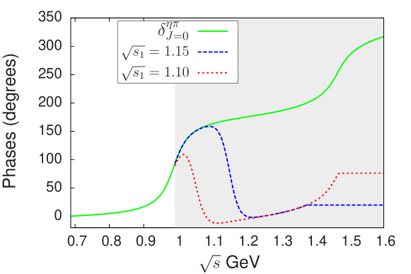
Figure 9: The solid line is the $l=0$ $\pi\eta$ scattering phase shift obtained from the model of ref. [41], the shaded area indicates the region where scattering is inelastic. The dashed lines shows the scalar form factor phase $\phi^{\eta\pi}$ for two values of $s_{1}$ (see text).

Above the $K\bar{K}$ threshold, $\eta\pi$ scattering becomes inelastic under the effect, mainly, of the two-body channels $K\bar{K}$ and $\eta^{\prime}\pi$. The phase $\phi^{\eta\pi}$ must then differ from $\delta_{0}^{\eta\pi}$. A global constraint on $\phi^{\eta\pi}$ arises from imposing that the form factor, as given from eq. (85), exhibits no exponential divergence asymptotically. This gives rise to a sum rule

$$\zeta\equiv{\dot{f}^{\eta\pi}_{0}(0)\over f^{\eta\pi}_{0}(0)}={1\over\pi}\int_{(m_{\eta}+m_{\pi})^{2}}^{\infty}{\phi^{\eta\pi}(s^{\prime})\over(s^{\prime})^{2}}\,ds^{\prime}\ .$$ (90)

Using the chiral expansion results for $\zeta$ (see sec. 3.3), the sum rule indicates that one should have $\phi^{\eta\pi}<<\delta_{0}^{\eta\pi}$ in the inelastic region. In order to estimate more precisely how $\phi^{\eta\pi}$ behaves, one may rely on an analogy with the phase of the $K\pi$ scalar form factor. In that case, there is enough experimental information on the elastic as well as the leading two-body inelastic $T$-matrix elements, such that the form factor can be deduced from solving a set of Muskhelishvili-Omnès equations. The analysis performed in ref. [80] shows that the form factor phase displays a sharp drop shortly after the onset of the leading inelastic channel. A similar behaviour has been also observed in the case of the $\pi\pi$ scalar form factor associated with the $\bar{u}u+\bar{d}d$ operator [82]. The authors argue that the presence of this phase drop is necessary in order to reproduce the correct value of the pion scalar radius via a sum rule analogous to eq. (90). We then propose the following simple model for the phase $\phi^{\eta\pi}$ assuming a fast decrease at $s=s_{1}$ and a constant value for $s>s_{2}$ with $4m_{K}^{2}<s_{1}<s_{2}$:

$$\begin{array}[]{ll}s\leq s_{2}:&\phi^{\eta\pi}(s)=\delta_{0}^{\eta\pi}(s)-\pi\theta(s-s_{1})\\ s>s_{2}:&\phi^{\eta\pi}(s)=\phi^{\eta\pi}(s_{2})\\ \end{array}$$ (91)

(a slight smoothing of the $\theta$ function is implemented in practice). For each value of $s_{1}$, the value of $s_{2}$ is determined such that the sum rule (90) is exactly satisfied. Fig. 9 illustrates the behaviour of $\phi^{\eta\pi}$ with $\sqrt{s_{1}}=1.05,\ 1.15$ GeV. In this model, $s_{1}$ is bounded from above: $\sqrt{s_{1}}<1.2$ GeV for otherwise, it is not possible to satisfy the sum rule (90).

6.2 Results for $f^{\eta\pi}_{0}$

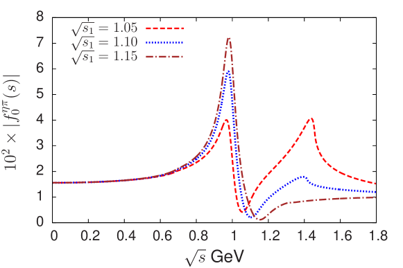
Figure 10: Modulus of the scalar form factor from the phase dispersive representation (85) and the phase model described in the text, for several values of the dip position $s_{1}$.

Using the phase $\phi^{\eta\pi}$ as described above, one can compute the scalar form factor from the dispersive representation (85). Results are shown in fig 10 for several values of $s_{1}$. The point $s_{1}$, where the phase drops, corresponds to a dip in the modulus of the form factor. Obviously, if the dip is located very close to the $K\bar{K}$ threshold, the peak of the $a_{0}(980)$ resonance is strongly reduced. This corresponds, in this approach, to a reduced coupling of the resonance to the $\bar{u}d$ scalar operator and thus to an exotic nature of the $a_{0}(980)$. One may formally define a coupling constant from the matrix element of the vector current involving the $a_{0}$ state [83]

$${\langle 0|j_{\mu}^{ud}|a_{0}^{-}(p)\rangle}=\sqrt{2}F_{a_{0}}p^{\mu}\ .$$ (92)

In a dispersive approach, it is in principle possible to identify such a coupling constant from the residue of the $a_{0}$ resonance pole of the scalar form factor on the second Riemann sheet. In a simpler way, one may obtain an estimate by matching the shape of the dispersive form factor with a Breit-Wigner-type shape. For this purpose, we have used the chiral resonance approach of ref. [23] in which one can vary the value of $F_{a_{0}}$ (via that of an $O(p^{6})$ chiral coupling constant, $d_{r}$) while the value of the form factor at the origin is kept fixed. In this manner, from the phase dispersive representation, with the largest allowed value of the dip parameter, we find

$$F_{a_{0}}\simeq 0.62\ \hbox{MeV}\$$ (93)

which thus represents an upper bound for this coupling in the present model. For comparison, based on QCD sum rules, values in the range $[0.8-1.6]$ MeV have been quoted [84, 83]. In the same framework, it was found in ref. [85] that, on the contrary, the $a_{0}$ coupling should be strongly suppressed, while estimates based on the bag model give a range of $[0.2-2.0]$ MeV [86]. A result from a lattice QCD simulation with $N_{f}=2$ dynamical quarks has been given [87], which corresponds to $F_{a_{0}}=[0.8-0.9]$ MeV.

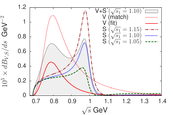
Figure 11: Contributions to the invariant mass distribution of the $\tau\to\eta\pi\nu$ branching fraction from the vector (V) and the scalar (S) form factors. For the vector contribution, the upper dotted curve corresponds to polynomial parameters from ChPT matching and the lower solid curve to parameters fitted to experiment. The scalar contribution is shown for several values of the dip parameter $s_{1}$. The shaded area shows a plausible central value for the sum of the two contributions .

7 Application to the $\tau\to\eta\pi\nu$ and $\eta_{l3}$ decays

We can now compute the contributions from the vector and scalar form factors to the differential decay width of the $\tau$ into $\eta\pi\nu$ (the relevant formula was given in eq. (7)). Fig. 11 shows the contribution from the vector form factor calculated from a KT amplitude with fitted polynomial parameters (lower curve) and that associated with parameters determined from ChPT matching (upper curve). The vector contribution is somewhat suppressed here by the kinematics but our calculations suggest that it should lead to a clearly visible $\rho$-meson peak. The contribution to the differential decay width from the scalar form factor is shown for three different values of the dip $s_{1}$.

The corresponding values for the integrated branching fraction of the $\tau\to\eta\pi\nu$ mode are given in table 3 and compared with some former results found in the literature. We quote here a plausible central value only, which corresponds to $\sqrt{s_{1}}=1.10$ GeV for the scalar form factor and to fitted polynomial parameters for the vector form factor. It is difficult to precisely evaluate the error, in particular in the case of the scalar form factor, because of the various assumptions and model dependence involved. A plausible guess however, in our approach, is that the scalar contribution to the branching fraction should lie in the range $0.1\cdot 10^{-5}\leq B_{S}\leq 0.6\cdot 10^{-5}$. This tends to be smaller than most previous estimates which are often based on simple scalar-dominance models. Conversely, in the dispersive approach, it seems difficult to accommodate a value for $B_{S}$ as small as quoted in ref. [34] even if the position of the dip $s_{1}$ is very close to the $K\bar{K}$ threshold, because of the contribution from below the resonance region.

In the case of the vector contribution, in view of some possible shifts in the experimental value of the $\eta\to 3\pi$ Dalitz plot parameters (see [68], p.16), a plausible range for the branching fraction should be: $0.10\cdot 10^{-5}\leq B_{V}\leq 0.40\times 10^{-5}$.

$10^{5}\times B_{V}$	$10^{5}\times B_{S}$	$10^{5}\times B_{V+S}$	ref.
0.25	1.60	1.85	Tisserant, Truong (1982)[29]
0.12	1.38	1.50	Pich (1987) [30]
0.15	1.06	1.21	Neufeld, Rupertsberger(1995)[23]
0.36	1.00	1.36	Nussinov, Soffer (2008)[32]
$[$0.2-0.6$]$	$[$0.2-2.3$]$	$[$0.4-2.9$]$	Paver, Riazuddin (2010)[33]
0.44	0.04	0.48	Volkov,Kostunin (2012)[34]
0.13	0.20	0.33	Present work

Table 3: Theoretical estimates of the branching fraction of the $\tau\to\eta\pi\nu$ mode, showing the separate contribution from the vector and scalar form factors. The central values from the approach used here are shown on the last line.

Finally, for the $\eta_{l3}$ decays, we find the following central values for the branching fractions (adding the two charge modes)

$$\begin{array}[]{l}B_{\eta\to\pi^{+}e^{-}\nu+c.c.}\simeq 1.40\times 10^{-13}\\ B_{\eta\to\pi^{+}\mu^{-}\nu+c.c.}=1.02\times 10^{-13}\\ \end{array}$$ (94)

The results, in this case, are practically identical to those computed with the chiral NLO form factors[23, 24]. An experimental upper bound on the $\eta_{e3}$ mode branching fraction has been obtained recently by the BESIII [88] collaboration

$$B_{\eta\to\pi^{+}e^{-}\nu+c.c.}<1.7\times 10^{-4}\ .$$ (95)

8 Conclusions

In this work, we have reconsidered the $\eta\pi$ isospin-violating vector and scalar form factors and the related energy distribution in the second-class $\tau\to\eta\pi\nu$ decay which should be measurable at future $B$ or $\tau$-charm factories. We have started from the NLO ChPT results for $f^{\eta\pi}_{+}(0)$ and for the derivatives $\dot{f}^{\eta\pi}_{+}(0)$, $\dot{f}^{\eta\pi}_{0}(0)$. In particular, for $f^{\eta\pi}_{+}(0)$ a relation was established [23] with the $K^{+}_{l3}$ and $K^{0}_{l3}$ decays which can now be used thanks to recent experimental progress [49]. These results at $s=0$ could be checked, in principle, in lattice QCD simulations including isospin violation.

In order to evaluate the form factors in the resonance regions we further relied on their analyticity properties. We argued that these should be the same as in the more familiar cases of the $\pi\pi$ or the $\pi K$ form factors, i.e., no anomalous threshold should be present despite the fact that the $\eta$ meson is unstable. Its instability only generates a few technical complications in the case of $f^{\eta\pi}_{+}$: the discontinuity along the unitarity cut is complex and, furthermore, it displays a divergence at the pseudothreshold $s=(m_{\eta}-m_{\pi})^{2}$.

Below 1 GeV, the essential contribution to the discontinuity is proportional to the $\eta\pi\to\pi\pi$ amplitude, projected on the $P$-wave. We constructed a four-parameter family of solutions of the Khuri-Treiman equations which we use in the dispersion relation for $f^{\eta\pi}_{+}$. The shape of the vector form factor, in particular the $\rho$-meson peak, is then correlated with the Dalitz plot parameters of the $\eta\to 3\pi$ amplitude (in particular, the parameter $d$). Upon using the recent experimental constraints for the Dalitz plot, we find the $\rho$-meson peak to be suppressed as compared with earlier evaluations and that its shape differs from the naive vector dominance model.

In the case of the scalar form factor $f^{\eta\pi}_{0}$, we used a phase dispersive representation. For the $\eta\pi$ scattering phase shift in the elastic region, we relied on the $\eta\pi$ scattering model proposed in ref. [41]. This model should be reasonable, at the qualitative level, but it is clear that there is much to be improved on our knowledge of $\eta\pi$ scattering. Again in this case, lattice QCD simulations which are making steady progress in evaluating meson-meson interactions (see [89] for recent work), could provide unique information, e.g., on the value of the scattering length.

At energies above the $K\bar{K}$ threshold, we argued that a plausible behaviour for the phase is that it should display a sharp fall-off (which corresponds to a dip in the modulus), by analogy with the cases of the $\pi\pi$ or the $\pi K$ scalar form factors, where the corresponding phase can be generated from dynamical models. In this approach the exotic (non-exotic) nature of the $a_{0}(980)$ resonance corresponds to the dip being situated close (far) from the resonance position. This feature of the phase can then be used in association with a global constraint from a sum rule, which relates the integral over the phase to the logarithmic derivative of the form factor at the origin. Varying the position of the dip generates the main source of uncertainty in this approach. The sum rule restricts the range of variation of the dip but the uncertainties still remain much larger than the $20\%$ level required to make the $\tau\to\eta\pi\nu$ process competitive for constraining the parameters of particle physics models involving charged Higgs bosons.

Appendix A Angular projection kernels

In sec. 5.2 the angular integrals of the functions $M_{I}(t(s,z))$ were expressed in terms of kernels. The kernels needed for $I=1$, firstly, have the following expression

$$P^{(0)}(t^{\prime},s)={1\over t^{\prime}}+L(t^{\prime},s)$$

$$P^{(1)}(t^{\prime},s)={2\over\kappa(s)}+{(2t^{\prime}+s-3s_{0})\over\kappa(s)}\,L(t^{\prime},s)$$

$$P^{(2)}(t^{\prime},s)={1\over 3t^{\prime}}+{2(2t^{\prime}+s-3s_{0})\over\kappa(s)^{2}}+{(2t^{\prime}+s-3s_{0})^{2}\over\kappa(s)^{2}}\,L(t^{\prime},s)\ ,$$ (96)

where the logarithmic function $L(t^{\prime},s)$ was given in eq. (70). For $I=0,2$ the two kernels which are needed read

$$K^{(0)}(t^{\prime},s)={3s_{0}-s\over 2(t^{\prime})^{2}}+P^{(0)}(t^{\prime},s)$$

$$K^{(1)}(t^{\prime},s)={\kappa(s)\over 6(t^{\prime})^{2}}+P^{(1)}(t^{\prime},s)$$ (97)

Appendix B Verification of the $O(p^{4})$ discontinuities

Let us verify here, using the general unitarity formulae for $f^{\eta\pi}_{+}(s)$ and $f^{\eta\pi}_{0}(s)$ given in secs. 2.1 and 2.2 that one reproduces the $O(p^{4})$ results. For this purpose, one must use the chiral expansions of the form factors and those of the scattering amplitudes which appear in the unitarity relations at order $p^{2}$. The expressions for the three relevant scattering amplitudes at $O(p^{2})$ are

$$T_{\eta{\pi^{+}}\to{\pi^{0}}{\pi^{+}}}(s,t,u)=-\epsilon\,{3t-4m_{\pi}^{2}\over 3F_{0}^{2}},$$

$$T_{\eta{\pi^{+}}\to\eta{\pi^{+}}}(s,t,u)={m_{\pi}^{2}\over 3F_{0}^{2}}$$

$$T_{\eta{\pi^{+}}\to{\bar{K}^{0}}{K^{+}}}(s,t,u)={\sqrt{6}(3s-4m_{K}^{2})\over 12F_{0}^{2}}+\sqrt{2}\epsilon{t-u\over 4F_{0}^{2}}\ .$$ (98)

The unitarity relation for $f^{\eta\pi}_{+}$ involves the $l=1$ partial-wave projections of these amplitudes which read

$${1\over 2}\int_{-1}^{1}dzz\,T_{\eta{\pi^{+}}\to{\pi^{0}}{\pi^{+}}}=-\epsilon\,\sqrt{{s-4m_{\pi}^{2}\over s}}\,{\sqrt{\lambda_{\eta\pi}(s)}\over 6F_{0}^{2}},\$$

$${1\over 2}\int_{-1}^{1}dzz\,T_{\eta{\pi^{+}}\to{\bar{K}^{0}}{K^{+}}}=\sqrt{2}\epsilon\,\sqrt{{s-4m_{K}^{2}\over s}}\,{\sqrt{\lambda_{\eta\pi}(s)}\over 12F_{0}^{2}}\ .$$ (99)

while the $l=1$ projection of $T_{\eta{\pi^{+}}\to\eta{\pi^{+}}}$ vanishes. Using also that the vector form factors $F_{V}^{\pi}=F_{V}^{K}=1$ at $O(p^{2})$, one easily finds from the unitarity relations of sec. 2.1

$${\rm Im\,}f^{\eta\pi}_{+}(s)=\epsilon{(s-4m_{\pi}^{2})\over 6F_{0}^{2}}{\rm Im\,}\bar{J}_{\pi\pi}(s)+\epsilon{(s-4m_{K}^{2})\over 12F_{0}^{2}}{\rm Im\,}\bar{J}_{KK}(s)\ .$$ (100)

Analogously, the unitarity relation for $f^{\eta\pi}_{0}$ involves the $l=0$ partial-wave projections

$${1\over 2}\int_{-1}^{1}dz\,T_{\eta{\pi^{+}}\to\pi^{0}{\pi^{+}}}=\epsilon{3s-4m_{K}^{2}\over 6F_{0}^{2}}$$

$${1\over 2}\int_{-1}^{1}dz\,T_{\eta{\pi^{+}}\to\eta{\pi^{+}}}={m_{\pi}^{2}\over 3F_{0}^{2}}$$

$${1\over 2}\int_{-1}^{1}dz\,T_{\eta{\pi^{+}}\to{\bar{K}^{0}}{K^{+}}}=\sqrt{6}\,{3s-4m_{K}^{2}\over 12F_{0}^{2}}\ .$$ (101)

Using the unitarity relations in sec. 2.2 and the $O(p^{2})$ expressions for the scalar form factors $f_{0}^{\pi\pi}=f_{0}^{KK}=1$ and $f_{0}^{\eta\pi}=\epsilon$, one obtains

$${\rm Im\,}f^{\eta\pi}_{0}(s)=-\epsilon{\Delta_{{\pi^{0}}{\pi^{+}}}\over\Delta_{\eta\pi^{+}}}{(3s-4m_{K}^{2})\over 6F_{0}^{2}}{\rm Im\,}\bar{J}_{\pi\pi}(s)$$

$$\phantom{{\rm Im\,}f^{\eta\pi}_{0}(s)}+\epsilon{m_{\pi}^{2}\over 3F_{0}^{2}}{\rm Im\,}\bar{J}_{\eta\pi}(s)+{\Delta_{K^{0}K^{+}}\over\Delta_{\eta\pi}}{\sqrt{3}(3s-4m_{K}^{2})\over 12F_{0}^{2}}{\rm Im\,}\bar{J}_{KK}(s)\ .$$ (102)

Dropping the double isospin-suppressed term and expanding $\Delta_{K^{0}K^{+}}=m^{2}_{K^{0}}-m^{2}_{K^{+}}$ at $O(p^{2})$ and $O(e^{2})$ one recovers exactly the imaginary part of the $O(p^{4})$ formula (44).

Appendix C Dalitz plot parameters

For the charged decay, $\eta\to\pi^{+}\pi^{-}\pi^{0}$, a point inside the Dalitz plot may be determined in terms of two coordinates $X$,$Y$ defined as

$$X=\sqrt{3}{T_{{\pi^{+}}}-T_{{\pi^{-}}}\over Q_{c}},\quad Y=3{T_{{\pi^{0}}}\over Q_{c}}-1$$ (103)

where $T_{\pi_{i}}=p^{0}_{\pi_{i}}-m_{\pi_{i}}$ is the kinetic energy of the pion $\pi_{i}$ in the $\eta$ rest frame and $Q_{c}=\sum_{i}T_{\pi_{i}}=m_{\eta}-2m_{\pi^{+}}-m_{\pi^{0}}$. In terms of the Mandelstam variables, one has

$$X={\sqrt{3}(u-t)\over 2m_{\eta}Q_{c}},\quad Y={3((m_{\eta}-m_{\pi^{0}})^{2}-s)\over 2m_{\eta}Q_{c}}-1\ .$$ (104)

The Dalitz plot coefficients parametrise the variation of the square of the amplitude from the center of the plot

$$\rho_{c}(X,Y)={|{\cal M}_{c}(X,Y)|^{2}\over|{\cal M}_{c}(0,0)|^{2}}=1+aY+bY^{2}+dX^{2}+fY^{3}+GX^{2}Y+\cdots\ .$$ (105)

The parametrisation accounts for the invariance of the amplitude under the transformation $X\to-X$ which results from charge conjugation invariance.

In the case of the decays into three neutral pions one similarly introduces two variables

$$X=\sqrt{3}{T_{\pi^{0}_{1}}-T_{\pi^{0}_{2}}\over Q_{n}},\quad Y=3{T_{\pi^{0}_{3}}\over Q_{n}}-1$$ (106)

with $Q_{n}=m_{\eta}-3m_{\pi^{0}}$. The amplitude is invariant under Bose symmetry transformations $\pi^{0}_{i}\leftrightarrow\pi^{0}_{j}$. Using eq. (106), one deduces that it must be invariant under the following transformations of the $X$, $Y$ variables

$$X\to-X,\quad(X+iY)\to\exp({-i\pi\over 3})(X-iY)\ .$$ (107)

The expansion of the amplitude squared around the center of the Dalitz plot thus has the form,

$$\rho_{n}(X,Y)={|{\cal M}_{n}(X,Y)|^{2}\over|{\cal M}_{n}(0,0)|^{2}}=1+2\alpha(X^{2}+Y^{2})+2\gamma(3X^{2}Y-Y^{3})+\cdots\ .$$ (108)

Appendix D Second-class amplitude in $\tau\to\pi^{0}\pi^{+}\nu$ decay

We remark here that the $\pi\pi$ scalar form factor $f_{0}^{\pi\pi}$ (see eq. (20)), while involving no resonance contribution (to first order in isospin breaking) can be estimated in an essentially model independent way in the low-energy region. The $\pi^{0}\pi^{+}$ system with $l=0$ must be in an isospin $I=2$ state. From Watson’s theorem, the phase of the scalar form factor $\phi_{0}$, must coincide with the $l=0$, $I=2$ $\pi\pi$ scattering phase shift $\delta_{0}^{2}$ in an energy range $s<s_{in}\simeq 1\ \hbox{GeV}^{2}$ where $\pi\pi$ scattering is elastic to a good approximation. We can then express $f_{0}^{\pi\pi}$ as a phase dispersive representation,

$$f_{0}^{\pi\pi}(s)=\exp\left({s\over\pi}\int_{4m_{\pi}^{2}}^{\infty}ds^{\prime}{\delta_{0}^{2}(s^{\prime})\over s^{\prime}(s^{\prime}-s)}\right)\exp\left({s\over\pi}\int_{s_{in}}^{\infty}ds^{\prime}{\phi_{0}(s^{\prime})-\delta_{0}^{2}(s^{\prime})\over s^{\prime}(s^{\prime}-s)}\right)\$$ (109)

(using that $f_{0}^{\pi\pi}(0)=F_{V}^{\pi}(0)=1$). At energies $s<<s_{in}$ we can neglect the effect of the second exponential in eq. (109) and thus obtain an approximation of the form factor in terms of the known $I=2$ phase shift.

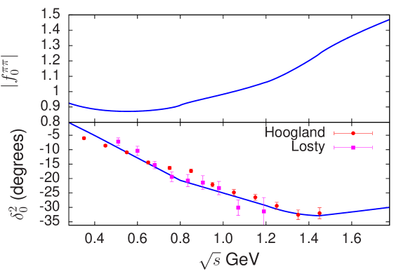
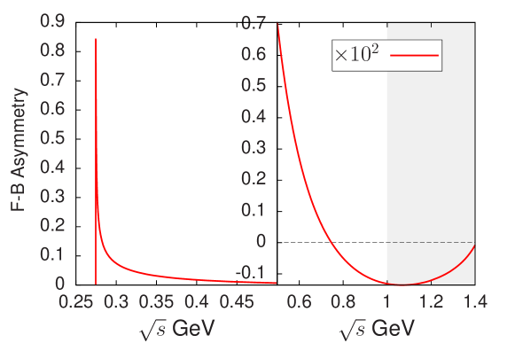
Figure 12: The upper figure shows the $I=2$ $S$-wave $\pi\pi$ phase shift (the experimental data are taken from refs. [90, 91]) and the scalar form factor from eq. (109), neglecting the second exponential. The lower figure shows the forward-backward asymmetry in the $\tau\to\pi^{0}\pi^{+}\nu$ decay as a function of the $\pi\pi$ energy. The shaded area indicates the region where the calculation becomes unreliable.

The form factor $f_{0}^{\pi\pi}$ plays a role in the search for CP violation [92]. Let us consider here its effect in generating a forward-backward asymmetry in the $\tau\to\pi^{0}\pi^{+}\nu$ decay,

$${\cal A}_{\pi\pi}(s)=\dfrac{\int_{0}^{1}d\cos\theta{d^{2}\Gamma\over dsd\cos\theta}-\int_{-1}^{0}d\cos\theta{d^{2}\Gamma\over dsd\cos\theta}}{\int_{0}^{1}d\cos\theta{d^{2}\Gamma\over dsd\cos\theta}+\int_{-1}^{0}d\cos\theta{d^{2}\Gamma\over dsd\cos\theta}}$$ (110)

where $\theta$ is the angle between the three-momenta of the $\pi^{+}$ and the $\tau$ in the $\pi\pi$ center-of-mass system. In the energy range $s<s_{in}$ one can express the FB asymmetry in terms of the moduli of the form factors and the $I=1,2$ phase shifts,

$${\cal A}_{\pi\pi}(s)=\dfrac{3\Delta_{{\pi^{+}}{\pi^{0}}}\sqrt{\lambda_{{\pi^{+}}{\pi^{0}}}(s)}|F_{V}^{\pi}(s)||f_{0}^{\pi\pi}(s)|\cos(\delta_{1}^{1}-\delta_{0}^{2})}{|F_{V}^{\pi}(s)|^{2}\lambda_{{\pi^{+}}{\pi^{0}}}(s)(1+{2s/m_{\tau}^{2}})+3|f_{0}^{\pi\pi}(s)|^{2}\Delta^{2}_{{\pi^{+}}{\pi^{0}}}}\ .$$ (111)

Fig. 12 shows that the asymmetry is very small except however in the energy region $\sqrt{s}\leq 300$ MeV where it is positive and larger that 10%.

References

- [1] R.F. Dashen, Phys.Rev. 183, 1245 (1969)
- [2] D. Sutherland, Phys.Lett. 23, 384 (1966)
- [3] R. Baur, J. Kambor, D. Wyler, Nucl.Phys. B460, 127 (1996), hep-ph/9510396
- [4] A. Deandrea, A. Nehme, P. Talavera, Phys.Rev. D78, 034032 (2008), 0803.2956
- [5] C. Ditsche, B. Kubis, U.G. Meissner, Eur.Phys.J. C60, 83 (2009), 0812.0344
- [6] C. Adolph et al. (WASA-at-COSY), Phys.Lett. B677, 24 (2009), 0811.2763
- [7] M. Unverzagt et al. (Crystal Ball at MAMI , TAPS , A2), Eur.Phys.J. A39, 169 (2009), 0812.3324
- [8] S. Prakhov et al. (Crystal Ball at MAMI, A2), Phys.Rev. C79, 035204 (2009), 0812.1999
- [9] F. Ambrosino et al. (KLOE), Phys.Lett. B694, 16 (2010), 1004.1319
- [10] F. Ambrosino et al. (KLOE), JHEP 0805, 006 (2008), 0801.2642
- [11] J. Gasser, H. Leutwyler, Nucl.Phys. B250, 539 (1985)
- [12] J. Bijnens, K. Ghorbani, JHEP 0711, 030 (2007), 0709.0230
- [13] K. Kampf, M. Knecht, J. Novotny, M. Zdrahal, Phys.Rev. D84, 114015 (2011), 1103.0982
- [14] S.P. Schneider, B. Kubis, C. Ditsche, JHEP 1102, 028 (2011), 1010.3946
- [15] C. Roiesnel, T.N. Truong, Nucl.Phys. B187, 293 (1981)
- [16] N. Khuri, S. Treiman, Phys.Rev. 119, 1115 (1960)
- [17] A. Neveu, J. Scherk, Annals Phys. 57, 39 (1970)
- [18] J. Kambor, C. Wiesendanger, D. Wyler, Nucl.Phys. B465, 215 (1996), hep-ph/9509374
- [19] A. Anisovich, H. Leutwyler, Phys.Lett. B375, 335 (1996), hep-ph/9601237
- [20] G. Colangelo, S. Lanz, H. Leutwyler, E. Passemar, PoS EPS-HEP2011, 304 (2011)
- [21] S. Lanz, PoS CD12, 007 (2013), 1301.7282
- [22] H. Leutwyler, Mod.Phys.Lett. A28, 1360014 (2013), 1305.6839
- [23] H. Neufeld, H. Rupertsberger, Z.Phys. C68, 91 (1995)
- [24] D. Scora, K. Maltman, Phys.Rev. D51, 132 (1995)
- [25] S. Weinberg, Phys.Rev. 112, 1375 (1958)
- [26] J.E. Bartelt et al. (CLEO), Phys.Rev.Lett. 76, 4119 (1996)
- [27] P. del Amo Sanchez et al. (BaBar), Phys.Rev. D83, 032002 (2011), 1011.3917
- [28] K. Hayasaka (Belle Collaboration), PoS EPS-HEP2009, 374 (2009)
- [29] S. Tisserant, T. Truong, Phys.Lett. B115, 264 (1982)
- [30] A. Pich, Phys.Lett. B196, 561 (1987)
- [31] V. Bednyakov, Phys.Atom.Nucl. 56, 86 (1993)
- [32] S. Nussinov, A. Soffer, Phys.Rev. D78, 033006 (2008), 0806.3922
- [33] N. Paver, Riazuddin, Phys.Rev. D82, 057301 (2010), 1005.4001
- [34] M. Volkov, D. Kostunin, Phys.Rev. D86, 013005 (2012), 1205.3329
- [35] D. Asner, T. Barnes, J. Bian, I. Bigi, N. Brambilla et al., Int.J.Mod.Phys. A24, S1 (2009), 0809.1869
- [36] A. Bondar (Charm-Tau Factory), Phys.Atom.Nucl. 76(9), 1072 (2013)
- [37] A. Akeroyd et al. (SuperKEKB Physics Working Group) (2004), hep-ex/0406071
- [38] A. Bramon, S. Narison, A. Pich, Phys.Lett. B196, 543 (1987)
- [39] A. Pich, P. Tuzon, Phys.Rev. D80, 091702 (2009), 0908.1554
- [40] M. Jung, A. Pich, P. Tuzon, JHEP 1011, 003 (2010), 1006.0470
- [41] D. Black, A.H. Fariborz, J. Schechter, Phys.Rev. D61, 074030 (2000), hep-ph/9910351
- [42] A. Sirlin, Rev.Mod.Phys. 50, 573 (1978)
- [43] J. Erler, Rev.Mex.Fis. 50, 200 (2004), hep-ph/0211345
- [44] V. Cirigliano, M. Knecht, H. Neufeld, H. Rupertsberger, P. Talavera, Eur.Phys.J. C23, 121 (2002), hep-ph/0110153
- [45] J. Gasser, H. Leutwyler, Nucl.Phys. B250, 465 (1985)
- [46] R. Urech, Nucl.Phys. B433, 234 (1995), hep-ph/9405341
- [47] H. Neufeld, H. Rupertsberger, Z.Phys. C71, 131 (1996), hep-ph/9506448
- [48] B. Ananthanarayan, B. Moussallam, JHEP 0205, 052 (2002), hep-ph/0205232
- [49] M. Antonelli, V. Cirigliano, G. Isidori, F. Mescia, M. Moulson et al., Eur.Phys.J. C69, 399 (2010), 1005.2323
- [50] S. Aoki, Y. Aoki, C. Bernard, T. Blum, G. Colangelo et al. (FLAG Working Group) (2013), 1310.8555
- [51] J. Bijnens, P. Talavera, JHEP 0203, 046 (2002), hep-ph/0203049
- [52] C. Callan, S. Treiman, Phys.Rev.Lett. 16, 153 (1966)
- [53] R.F. Dashen, M. Weinstein, Phys.Rev.Lett. 22, 1337 (1969)
- [54] B. Ananthanarayan, B. Moussallam, JHEP 0406, 047 (2004), hep-ph/0405206
- [55] G. Barton, Introduction to dispersion techniques in field theory, Lecture notes and supplements in physics (W.A. Benjamin, New York, 1965)
- [56] J. Gasser, M. Sainio, Eur.Phys.J. C6, 297 (1999), hep-ph/9803251
- [57] S. Mandelstam, Phys.Rev.Lett. 4, 84 (1960)
- [58] R. Oehme, Phys.Rev. 6, 1840 (1961)
- [59] S. Lanz, Ph.D. thesis, University of Bern (2011)
- [60] J. Stern, H. Sazdjian, N. Fuchs, Phys.Rev. D47, 3814 (1993), hep-ph/9301244
- [61] J. Kennedy, T.D. Spearman, Phys.Rev. 126, 1596 (1961)
- [62] L. Muskhelishvili, N., Singular Integral Equations (P. Noordhof, Groningen, 1953)
- [63] R. Omnès, Nuovo Cim. 8, 316 (1958)
- [64] J. Bijnens, I. Jemos, Nucl.Phys. B854, 631 (2012), 1103.5945
- [65] B. Hyams, C. Jones, P. Weilhammer, W. Blum, H. Dietl et al., Nucl.Phys. B64, 134 (1973)
- [66] J. Batley et al. (NA48-2), Eur.Phys.J. C70, 635 (2010)
- [67] J. Beringer et al. (Particle Data Group), Phys.Rev. D86, 010001 (2012)
- [68] M. Amaryan, M. Bashkanov, M. Benayoun, F. Bergmann, J. Bijnens et al. (2013), 1308.2575
- [69] M. Fujikawa et al. (Belle Collaboration), Phys.Rev. D78, 072006 (2008), 0805.3773
- [70] G. Gounaris, J. Sakurai, Phys.Rev.Lett. 21, 244 (1968)
- [71] A. Duncan, A.H. Mueller, Phys.Rev. D21, 1636 (1980)
- [72] G.P. Lepage, S.J. Brodsky, Phys.Rev. D22, 2157 (1980)
- [73] V. Bernard, N. Kaiser, U.G. Meissner, Phys.Rev. D44, 3698 (1991)
- [74] A.H. Fariborz, J. Schechter, Phys.Rev. D60, 034002 (1999), hep-ph/9902238
- [75] B. Kubis, S.P. Schneider, Eur.Phys.J. C62, 511 (2009), 0904.1320
- [76] M. Kolesar, J. Novotny, Eur.Phys.J. C56, 231 (2008), 0802.1289
- [77] J. Oller, E. Oset, J. Pelaez, Phys.Rev. D59, 074001 (1999), hep-ph/9804209
- [78] N. Achasov, G. Shestakov, Phys.Rev. D81, 094029 (2010), 1003.5054
- [79] S. Uehara et al. (Belle), Phys.Rev. D80, 032001 (2009), 0906.1464
- [80] M. Jamin, J.A. Oller, A. Pich, Nucl.Phys. B622, 279 (2002), hep-ph/0110193
- [81] B. El-Bennich, A. Furman, R. Kaminski, L. Lesniak, B. Loiseau et al., Phys.Rev. D79, 094005 (2009), 0902.3645
- [82] B. Ananthanarayan, I. Caprini, G. Colangelo, J. Gasser, H. Leutwyler, Phys.Lett. B602, 218 (2004), hep-ph/0409222
- [83] S. Narison, Phys.Lett. B216, 191 (1989)
- [84] K. Maltman, Phys.Lett. B462, 14 (1999), hep-ph/9906267
- [85] V. Elias, A. Fariborz, F. Shi, T.G. Steele, Nucl.Phys. A633, 279 (1998), hep-ph/9801415
- [86] S. Fajfer, R. Oakes, Phys.Lett. B213, 376 (1988)
- [87] C. McNeile, C. Michael (UKQCD Collaboration), Phys.Rev. D74, 014508 (2006), hep-lat/0604009
- [88] M. Ablikim et al. (BESIII), Phys.Rev. D87(3), 032006 (2013), 1211.3600
- [89] C. Lang, L. Leskovec, D. Mohler, S. Prelovsek, Phys.Rev. D86, 054508 (2012), 1207.3204
- [90] M. Losty, V. Chaloupka, A. Ferrando, L. Montanet, E. Paul et al., Nucl.Phys. B69, 185 (1974)
- [91] W. Hoogland, S. Peters, G. Grayer, B. Hyams, P. Weilhammer et al., Nucl.Phys. B126, 109 (1977)
- [92] P. Avery et al. (CLEO), Phys.Rev. D64, 092005 (2001), hep-ex/0104009