subref \newrefsubname = section \RS@ifundefinedthmref \newrefthmname = theorem \RS@ifundefinedlemref \newreflemname = lemma
Extracting hadron masses from fixed
topology simulations
Arthur Dromard, Marc Wagner
Goethe-Universität Frankfurt am Main, Institut für Theoretische Physik,
Max-von-Laue-Straße 1, D-60438 Frankfurt am Main, Germany
July 16, 2014
Abstract
Lattice QCD simulations tend to become stuck in a single topological sector at fine lattice spacing or when using chirally symmetric overlap quarks. In such cases physical observables differ from their full QCD counterparts by finite volume corrections. These systematic errors need to be understood on a quantitative level and possibly be removed. In this paper we extend an existing relation from the literature between two-point correlation functions at fixed and the corresponding hadron masses at unfixed topology by calculating all terms proportional to and , where is the spacetime volume. Since parity is not a symmetry at fixed topology, parity mixing is comprehensively discussed. In the second part of this work we apply our equations to a simple model, quantum mechanics on a circle both for a free particle and for a square-well potential, where we demonstrate in detail, how to extract physically meaningful masses from computations or simulations at fixed topology.
1 Introduction
A QCD path integral includes the integration over all possible gauge or gluonic field configurations. These gauge field configurations can be classified according to their topological charge, which is integer. The numerical method to solve QCD path integrals is lattice QCD. In lattice QCD the path integral is simulated by randomly generating a representative set of gauge field configurations using Hybrid Monte Carlo (HMC) algorithms (cf. e.g. [1]). These algorithms modify a given gauge field configuration in a nearly continuous way. One of the key ideas of such a process is to generate almost exclusively gauge field configurations, which have small Euclidean action, i.e. which have a large weight and, therefore, dominate the path integral (importance sampling).
To simulate a QCD path integral correctly, it is essential to sample gauge field configurations from many topological sectors. A serious problem is, however, that topological sectors are separated by large action barriers, which increase, when decreasing the lattice spacing. As a consequence, common HMC algorithms are not anymore able to frequently change the topological sector for lattice spacings [2, 3], which are nowadays still fine, but within reach.
For some lattice discretizations, e.g. for chirally symmetric overlap quarks, the same problem arises already at much coarser lattice spacings. Such simulations are typically performed in a single topological sector, i.e. at fixed topological charge [4, 5], which introduces systematic errors. As an example one could mention [6], where different pion masses have been obtained for different topological charges and spacetime volumes. Those differences have to be quantified and, if not negligible compared to statistical errors, be removed.
There are also applications, where one might fix topology on purpose, either by sorting the generated gauge field configurations with respect to their topological charge or by directly employing so-called topology fixing actions (cf. e.g. [7, 8, 9]). For example, when using a mixed action setup with light overlap valence and Wilson sea quarks, approximate zero modes in the valence sector are not compensated by the sea. The consequence is an ill-behaved continuum limit [10, 11]. Since such approximate zero modes only arise at non-vanishing topological charge, fixing topology to zero might be a way to circumvent the problem.
In view of these issues it is important to study the relation between physical quantities (i.e. quantities corresponding to path integrals, where gauge field configurations from many topological sectors are taken into account) and correlation functions from fixed topology simulations.
In the literature one can find an equation describing the behavior of two-point correlation functions (suited to determine hadron masses) at fixed topology, derived up to first order and in part also to second order in ( is the topological susceptibility, is the spacetime volume) [12], and a general discussion of higher orders for arbitrary -point correlation functions at fixed topology [13]. In the first more theoretically oriented part of this work (sections 2 to 4) we extend the calculations from [12] by including all terms proportional to and . Since in many ensembles from typical nowadays lattice QCD simulations111In particular for expensive overlap quarks as well as for very small lattice spacings, where the problem of topology freezing is most severe, one is often restricted to rather small volumes , because of limited HPC resources. This in turn implies a small value of . (cf. e.g. [14, 15, 16, 17]), fixed topology corrections of order or even might be sizable. Another issue we address in detail is parity mixing in fixed topology two-point correlation functions. Since parity is not a symmetry at fixed topology, masses of negative and positive parity hadrons have to be extracted from the same correlation function or matrix (in the context of the meson this mixing has been observed and discussed in [13]). We also summarize all sources of systematic error and discuss the range of parameters (e.g. spatial and temporal extension of spacetime, topological charge, hadron masses), where the expansions of two-point correlation functions at fixed topology are accurate approximations.
In the second part of this work (section 5) we demonstrate, how to extract hadron masses from fixed topology simulations in practice. To this end we apply the previously obtained expansions of two-point correlation functions at fixed topology to a simple model, a quantum mechanical particle on a circle with and without potential. This model can be solved numerically up to arbitrary precision (there is no need to perform any simulations, only ordinary differential equations have to be solved) and, therefore, provides an ideal testbed. We have generated data points of correlation functions from many topological sectors and volumes and fit and compare different orders and versions of the previously derived correlator expansions. The results collected in various plots and tables are expected to provide helpful insights and guidelines for hadron mass determinations in quantum field theories, e.g. in QCD, at fixed topology (for related exploratory studies in the Schwinger model and the and non-linear Sigma model cf. [18, 19, 20, 21]).
2 The partition function at fixed topology and finite spacetime volume
In this section we calculate the dependence of the Euclidean QCD partition function at fixed topological charge on the spacetime volume , denoted as , up to .
2.1 Calculation of the expansion of
The Euclidean QCD partition function at non-vanishing angle and finite spacetime volume is defined as
| (2.1) |
[24] with
| (2.2) |
where is the periodic time extension, the spatial volume, , is the energy eigenvalue of the -th eigenstate of the Hamiltonian and the Euclidean QCD action without -term. Similarly, the Euclidean QCD partition function at fixed topological charge and finite spacetime volume is defined as
| (2.3) |
Using
| (2.4) |
it is easy to see that and are related by a Fourier transform,
| (2.5) |
One can show that [12], which implies . Using this together with (2.1) and (2.2) one can express the topological susceptibility, defined as
| (2.6) |
according to
| (2.7) |
(throughout this paper denotes the -th derivative of the quantity with respect to ). Moreover, we neglect ordinary finite volume effects, i.e. finite volume effects not associated with fixed topology. These are expected to be suppressed exponentially with increasing spatial volume (cf. section 4.2 for a discussion). In other words we assume to be sufficiently large such that , where is the energy density of the vacuum.
At sufficiently large the partition function is dominated by the vacuum, i.e.
| (2.8) |
where . The exponentially suppressed correction will be omitted in the following (cf. section 4.2 for a discussion). To ease notation, we define
| (2.9) |
Using also (2.8) the partition function at fixed topology (2.5) can be written according to
| (2.10) |
where the integral (2.10) can be approximated by means of the saddle point method. To this end, we expand around its minimum and replace by , which introduces another exponentially suppressed error (cf. section 4.2 for a discussion),
| (2.11) |
can be determined as a power series in . Due to , the expansion of the vacuum energy density around is
| (2.12) |
(note that ). Consequently,
| (2.13) |
It is straightforward to solve the defining equation for , , with respect to ,
| (2.14) |
Finally the saddle point method requires to deform the contour of integration to pass through the saddle point, which is just a constant shift of the real axis by the purely imaginary . We introduce the real coordinate parameterizing the shifted contour of integration yielding
| (2.15) |
After defining
| (2.16) |
a more compact notation for the result (2.15) is
| (2.17) |
where can also be written as
| (2.18) |
We now insert and (eqs. (2.13) and (2.14)) and perform the integration over order by order in (note that ). To this end we use the relations
| (2.19) | ||||
The terms in (2.18) are
-
•
for proportional to ,
-
•
for proportional to ,
-
•
for proportional to , …
Moreover, , , , … have to be even, otherwise the corresponding term in (2.18) vanishes, due to (2.19). Finally every odd and contributes in leading order in one power of . Therefore, up to it is sufficient to consider the following terms:
-
•
, :
(2.20) -
•
, :
(2.21) -
•
, :
(2.22) -
•
, :
(2.23) -
•
, :
(2.24) -
•
, , :
(2.25) -
•
, :
(2.26) -
•
, , :
(2.27) -
•
, , :
(2.28) -
•
, :
(2.29) -
•
, , :
(2.30) -
•
, :
(2.31) -
•
, , :
(2.32) -
•
, :
(2.33)
Inserting these expressions into (2.18) leads to
| (2.34) | ||||
and, after inserting the expansion of (2.14), yields
| (2.35) | ||||
2.2 Comparison with [12]
3 Two-point correlation functions at fixed topology and finite spacetime volume
In this section we derive a relation between physical hadron masses (i.e. at unfixed topology and ) and the corresponding two-point correlation functions at fixed topological charge and finite spacetime volume , denoted as , up to .
3.1 Calculation of the expansion of
Two-point correlation functions at fixed topological charge and finite spacetime volume are defined as
| (3.1) |
denotes a suitable hadron creation operator, for example for the charged pion a common choice is
| (3.2) |
(cf. e.g. [26] for an introduction in lattice hadron spectroscopy and the construction of hadron creation operators). is related to a corresponding two-point correlation function at non-vanishing angle and finite spacetime volume defined as
| (3.3) |
via a Fourier transform,
| (3.4) |
can be expressed in terms of energy eigenstates and eigenvalues,
| (3.5) |
When applied to the vacuum , the hadron creation operator creates a state, which has the quantum numbers of the hadron of interest , which are assumed to be not identical to those of the vacuum, even at . These states are denoted by , the corresponding eigenvalues by . is typically the lowest state in that sector333Note that parity is not a symmetry at . Therefore, states with defined parity at , which have lighter parity partners (e.g. positive parity mesons), have to be treated and extracted as excited states at and, consequently, also at fixed topology. This more complicated case is discussed in section 3.3., i.e. with mass (in this section we again neglect ordinary finite volume effects, i.e. finite volume effects not associated with fixed topology; cf. section 4.2 for a discussion). Using this notation one can rewrite (3.5) according to
| (3.6) | ||||
where and is the mass of the first excitation with the quantum numbers of .
For suitably normalized hadron creation operators , e.g. operators
| (3.7) |
where is a local operator, i.e. an operator exciting quark and gluon fields only at or close to , is independent of , i.e. . Moreover, for operators respecting either or , i.e. operators with defined parity , one can show by using , where is a non-unique phase. In the following we assume that is suitably normalized and has defined parity. Then can be written as a power series around according to
| (3.8) |
Inserting in (3.6) and neglecting exponentially suppressed corrections (cf. section 4.2 for a discussion) leads to
| (3.9) |
In analogy to (2.9) we define
| (3.10) |
For two-point correlation functions at fixed topology we then arrive at a similar form as for (eq. (2.10)),
| (3.11) |
With
| (3.12) |
the expansion of the exponent is
| (3.13) |
Up to its minimum can easily be obtained by using (2.14),
| (3.14) | ||||
can be written in the same form as (eq. (2.17)),
| (3.15) |
Using (2.35) and (2.38) yields an explicit expression up to ,
| (3.16) | ||||
with
| (3.17) | ||||
After inserting (eq. (2.38)), it is straightforward to obtain the final result for two-point correlation functions at fixed topology,
| (3.18) | ||||
where and are given in (2.35) and (3.17) (note that after inserting and in (3.18) the error is ). For some applications it might be helpful to have an expression for two-point correlation functions at fixed topology, which is of the form
| (3.19) |
i.e. where fixed topology effects only appear in the exponent and are sorted according to powers of . Such an expression can be obtained in a straightforward way from (3.18),
| (3.20) | ||||
Note that the order of the error is the same for both (3.18) and (3.20).
3.2 Comparison with [12]
3.3 Parity mixing
Parity is not a symmetry at . Therefore, states at cannot be classified according to parity and it is not possible to construct two-point correlation functions , where only or states contribute. Similarly, contains contributions both of states with or , since it is obtained by Fourier transforming (cf. (3.4)). Consequently, one has to determine the masses of and parity partners from the same two-point correlation functions444Note the similarity to twisted mass lattice QCD, where parity is also not an exact symmetry, and where and states are usually extracted from the same correlation matrix (cf. e.g. [27, 28, 29, 30, 31, 32, 33]).. While usually there are little problems for the lighter state (in the case of mesons typically the ground state), its parity partner (the ground state) has to be treated as an excitation. To precisely determine the mass of an excited state, a single correlator is in most cases not sufficient. For example to extract a first excitation it is common to study at least a correlation matrix formed by two hadron creation operators, which generate significant overlap to both the ground state and the first excitation.
We discuss the determination of and parity partners from fixed topology computations in a simple setup: a correlation matrix
| (3.23) |
with hadron creation operators and generating at unfixed topology and small mainly and , respectively. An example for such operators is
| (3.24) |
corresponding to the mesons and its parity partner . Without loss of generality we assume that the ground state (at ) has , denoted by , and the first excitation has , denoted by .
In the following we derive expressions for the four elements of the correlation matrix , . We proceed similar as in section 3.1. This time, however, we consider the two lowest states and (not only a single state),
| (3.25) |
(which is the generalization of (3.6) with exponentially suppressed corrections from higher excitations neglected), where
| (3.26) |
The overlaps of the trial states and the lowest states , and , have to be treated in a more general way, since the leading order of their expansion can be proportional to a constant, to or to depending on the indices , and . Since at parity is a symmetry, . Consequently,
-
•
, ,
while
-
•
, .
From the definition of (eq. (3.26)) one can conclude
-
•
, ,
-
•
, ,
-
•
, .
Using and , where is a non-unique phase, one can show
-
•
, (i.e. only even powers of in the corresponding expansions),
-
•
, (i.e. only odd powers of in the corresponding expansions).
Technically it is straightforward to consider not only the ground state , but also a first excitation : the contributions of the two states are just summed in (3.25), i.e. one can independently determine their Fourier transform and, hence, their contribution to the correlation matrix at fixed topology, . Additional calculations have to be done, however, for off-diagonal elements, where , and for contributions to diagonal matrix elements, where (cf. the following two subsections). Contributions to diagonal matrix elements, where , have already been determined (cf. section 3.1).
3.3.1 Calculation for , where
We proceed as in section 3.1. can be written as a power series around ,
| (3.27) |
The corresponding contribution to (cf. (3.25)) is
| (3.28) |
As before we define
| (3.29) |
For the contribution to the correlation matrix at fixed topology we then obtain
| (3.30) |
where is defined by (3.12) and (3.13). Consequently, its minimum is given by (3.14). (3.30) can be written as
| (3.31) | ||||
where is defined in (3.15) and
| (3.32) | ||||
As in section 2.1 it is easy to identify and calculate all terms of up to :
-
•
, ():
(3.33) -
•
, ():
(3.34) -
•
, , ():
(3.35)
Inserting these expressions into (3.32) leads to
| (3.36) |
The final explicit expression up to for the contribution to (eq. (3.31)) is
| (3.37) | ||||
After dividing by (eq. (2.38)), it is straightforward to obtain the final result. In exponential form (3.19) it is
| (3.38) | ||||
3.3.2 Calculation for , where
We proceed as in section 3.1. can be written as a power series around ,
| (3.39) |
The corresponding contribution to (cf. (3.25)) is
| (3.40) |
As before we define
| (3.41) |
For the contribution to the correlation matrix at fixed topology we then obtain
| (3.42) |
where is defined by (3.12) and (3.13). Consequently, its minimum is given by (3.14). (3.42) can be written as
| (3.43) | ||||
where is defined in (3.15), is defined in (3.32) and
| (3.44) | ||||
As in section 2.1 it is easy to identify and calculate all terms of up to :
-
•
():
(3.45) -
•
, ():
(3.46) -
•
, ():
(3.47) -
•
, , ():
(3.48)
Inserting these expressions into (3.44) leads to
| (3.49) |
3.3.3 The correlation matrix at fixed topology at
The correlation matrix , can be obtained by properly adding the results (3.20), (3.38) and (3.51). At first order in it is given by
| (3.52) | |||
| (3.53) | |||
| (3.54) |
where and (cf. (3.8)). The quantities are products of the more fundamental (cf. (3.26)) and, therefore, are not independent and fulfill certain constraints. Since the diagonal elements of are real and ,
-
•
and real (4 real parameters),
-
•
real (2 real parameters).
Moreover, from follows
-
•
and (4 real parameters).
Quite often one can define the hadron creation operators and in such a way that the off-diagonal elements of are real (or purely imaginary), which reduces the number of real parameters contained in from 10 to 8. There are further parameters, , , , and , i.e. in total 13 parameters.
(3.52) to (3.54) clearly show that parity mixing at fixed topology is already present at order . In particular this will cause problems, when trying to extract a hadron, which has a lighter parity partner, from a single two-point correlation function: e.g. the first term in (eq. (3.53)) is suited to determine a positive parity meson; however, there is a contamination by the corresponding lighter negative parity meson due to the second term, which is only suppressed proportional to with respect to the spacetime volume; since the first term is exponentially suppressed with respect to the temporal separation compared to the second term (), a precise determination of from the single correlator seems extremely difficult and would probably require extremely precise simulation results. Using the full correlation matrix (3.52) to (3.54) should, however, stabilize a fit to extract and at the same time (this is discussed in detail in section 5.3.4), similar to what is usually done at ordinary unfixed topology computations, when determining excited states.
This parity mixing at fixed topology has already been observed and discussed in the context of the meson in [13]. When considering the correlation function with a suitable meson creation operator, e.g.
| (3.55) |
one finds
| (3.56) |
where has been used ( is in this context the vacuum state). Using from [13] shows that there is a time independent contribution to the correlation function as in [13].
4 Discussion of errors
In this section we discuss, in which regime of parameters our expansions of two-point correlation functions at fixed topology (3.18) and (3.20) are accurate approximations.
4.1 Errors proportional to
In section 2.1 the spacetime dependence of two-point correlation functions has been derived up to . More precisely, the error is
| (4.1) |
(cf. (3.18), the text below (3.18) and (3.20)). This error will be small, if
-
(C1)
.
In other words, computations at fixed topology require large spacetime volumes (in units of the topological susceptibility ), while the topological charge may not be too large. We have also used , which requires
-
(C2)
.
The time dependence of this constraint excludes the use of large values of .
4.2 Exponentially suppressed errors
In sections 2.1 and 3.1 several exponentially suppressed corrections have been neglected:
-
(a)
Ordinary finite volume effects, i.e. finite volume effects not associated with fixed topology:
Such finite volume effects also appear in QCD simulations, where topology is not fixed. These effects are expected to be proportional to , where is the mass of the pion (the lightest hadron mass) and is the periodic spatial extension. -
(b)
Contributions of excited states to the partition function and to two-point correlation functions:
Excited states contribute to the partition function proportional to (cf. (2.8)), where is the mass of the lightest hadron, i.e. .
The corresponding dominating terms in a two-point correlation function are proportional to and (cf. (3.6)), where is the mass of the hadron of interest and the difference to its first excitation. - (c)
In zero temperature QCD simulations typically . For sufficiently large values of , e.g.
-
(C3)
as typically required in QCD simulations, corrections (a) and for the partition function also (b) should essentially be negligible. To be able to ignore corrections (b) for two-point correlation functions, one needs
-
(C4)
.
Corrections (c) can be neglected, if , which is already part of (C1).
For a discussion of the conditions (C1) to (C4) in the context of a numerical example cf. section 5.
5 Calculations at fixed topology in quantum mechanics
To test the equations derived in the previous sections, in particular (3.18) and (3.20), we study a simple model, quantum mechanics on a circle. It can be solved analytically or, in case of a potential, numerically up to arbitrary precision. We extract the difference of the two lowest energy eigenvalues, the equivalent of a hadron mass in QCD, from two-point correlation functions calculated at fixed topology. The insights obtained might be helpful for determining hadron masses from fixed topology simulations in QCD.
5.1 A particle on a circle in quantum mechanics
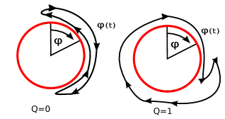
The Lagrangian of a quantum mechanical particle (mass ) on a circle (radius ) parameterized by the angle is
| (5.1) |
where is the moment of inertia. The potential will be specified below.
A periodic time with extension implies , , and gives rise to topological charge
| (5.2) |
The topological charge density is . Exemplary paths with topological charge and are sketched in Figure 5.1.
The path integral for the Euclidean partition function is
| (5.3) |
where the integration is over all paths, which are -periodic modulo , i.e. over all topological sectors.
The corresponding path integral over a single topological sector , which is relevant in the context of topology fixing, is
| (5.4) | ||||
(note that the analog of the spacetime volume in QCD is in quantum mechanics the temporal extension , i.e. throughout this section ). One can read off both and . The -dependent Hamiltonian, which can be obtained as usual, is
| (5.5) |
5.2 A free particle,
5.2.1 Eigenfunctions and eigenvalues
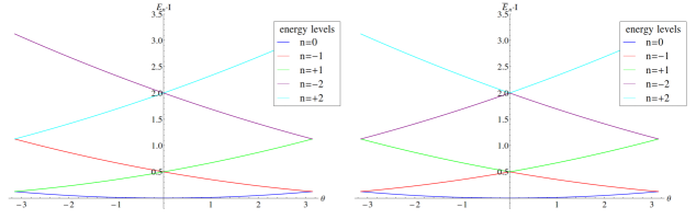
For the eigenfunctions and eigenvalues of can be determined analytically,
| (5.6) |
Note that in previous sections we used . While the spectrum fulfills this symmetry, it is clearly violated by our mathematical parameterization (5.6) for (cf. Figure 5.2, left plot). An equivalent set of eigenfunctions and eigenvalues fulfilling the symmetry is
| (5.7) |
(cf. Figure 5.2, right plot).
5.2.2 Partition function
The partition function is the Fourier transform of (cf. (5.4)). After inserting the eigenvalues and changing the variables of integration according to , one obtains a Gaussian integral, which is analytically solvable,
| (5.8) | ||||
5.2.3 Two-point correlation function
We use the creation operator (on a circle operators must be -periodic in ). Note that
- •
-
•
has non-vanishing overlap to the first excitation ,
i.e. is a suitable creation operator for the first excitation .
The two-point correlation function is the Fourier transform of , which can be expanded in terms of energy eigenstates (cf. (3.4) and (3.5)). After inserting the eigenvalues (eq. (5.6)), using and changing the variables of integration according to as in (5.8), one again obtains a Gaussian integral, which can be solved exactly,
| (5.10) |
The analog of the lightest hadron mass in QCD is the difference of the energy eigenvalues of the first excitation and the ground state,
| (5.11) |
Clearly , which implies . This in turn severely violates condition (C2) of section 4.1, which was assumed to be fulfilled, when deriving the approximations of two-point correlation functions (3.18) and (3.20). In other words, agreement between the exact result (5.10) and (3.18) and (3.20) cannot be expected and is neither observed.
To circumvent the problem, one can use the eigenvalue parameterization (5.6), which, however, does not fulfill . The consequence is that the expansion (3.13) may also contain odd terms , , etc. For a free particle, however, only few parameters are non-zero,
-
•
,
-
•
(the two lightest hadron masses need to be considered, since for and for ; cf. Figure 5.2)
, -
•
.
All further parameters , and vanish. Consequently, , and , while for . In other words in (3.13) there is only a single additional term, . Since this term is proportional to , and since there is already a term proportional to in (3.13), , it can easily be included in the calculation from section 3 by replacing and in (3.16), respectively, and by adding both results, to obtain . Inserting the above listed parameters and dividing by (eq. (5.9)) one finds
| (5.12) |
which is identical to the exact result (5.10), even though power corrections proportional to and exponentially suppressed corrections have been neglected.
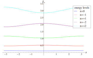
5.3 A particle in a square well
Now we study a square well potential
| (5.13) |
( is the depth and the width of the well). Again we use the creation operator , for which one can show 555A complicated theory like QCD has many symmetries and, therefore, many orthogonal sectors of states, which are labeled by the corresponding quantum numbers (total angular momentum, charge conjugation, flavor quantum numbers). In such a theory one typically chooses an operator exciting states, which do not have the quantum numbers of the vacuum, i.e. where , due to symmetry. In the simple quantum mechanical model parity is the only symmetry, which is broken at . Therefore, constructing an appropriate creation operator is less straightforward, because is not guaranteed by obvious symmetries, but has to be shown explicitly. (cf. appendix A.2).
5.3.1 Solving the model numerically
For the square well potential (5.13) the Schrödinger equation cannot be solved analytically, but numerically up to arbitrary precision, i.e. no simulations are required. For these numerical computations we express all dimensionful quantities in units of , i.e. we work with dimensionless quantities (denoted by a hat ) , and . For the numerical results presented in this section we have used and .
We proceeded as follows:
- 1.
- 2.
- 3.
-
4.
Perform a Fourier transformation numerically to obtain , the exact correlation function at fixed topology.
-
5.
Define and calculate the effective mass
(5.16)
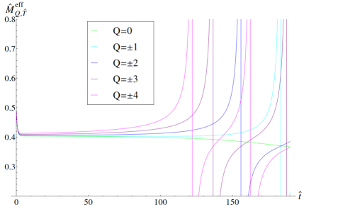
5.3.2 Effective masses at fixed topology
In Figure 5.4 we show effective masses (eq. (5.16)) as functions of the temporal separation for different topological sectors and . As usual at small temporal separations the effective masses are quite large and strongly decreasing, due to the presence of excited states. At large temporal separations there are also severe deviations from a constant behavior. This contrasts ordinary quantum mechanics or quantum field theory (i.e. at unfixed topology) and is caused by topology fixing. This effect is also visible in the expansion of the two point correlation function, in particular in (3.20), where the exponent is not purely linear in for large , but contains also terms proportional to and . At intermediate temporal separations there are plateau-like regions, which become smaller with increasing topological charge .
5.3.3 Comparison of the expansions of and the exact result
In Figure 5.5 we show effective masses derived from the expansions of two-point correlation functions666Note that in quantum mechanics a expansion is a expansion. (3.18) (left column) and (3.20) (right column) using the definition (5.16). The first, second and third row correspond to , and , respectively. To illustrate the relative importance of , and terms, we also show versions of (3.18) and (3.20), which are only derived up to and . While less accurate, these expressions contain a smaller number of parameters, which might be an advantage, when e.g. fitting to results from lattice simulations (such a fitting is discussed in section 5.3.4). In detail the following curves are shown with and the parameters taken from Table 1:
- •
- •
-
•
from (3.18) (which is derived up to );
14 parameters (, , , , , , , , , , , , , ). - •
- •
-
•
from (3.20) (which is derived up to );
11 parameters (, , , , , , , , , , ).
Note that the definition (5.16) of eliminates , i.e. effective masses have one parameter less than the corresponding two-point correlation functions. For comparison we also include the exact result already shown and discussed in Figure 5.4. Finally, the dashed line indicates the “hadron mass” at unfixed topology, to demonstrate the effect of topology fixing on effective masses.
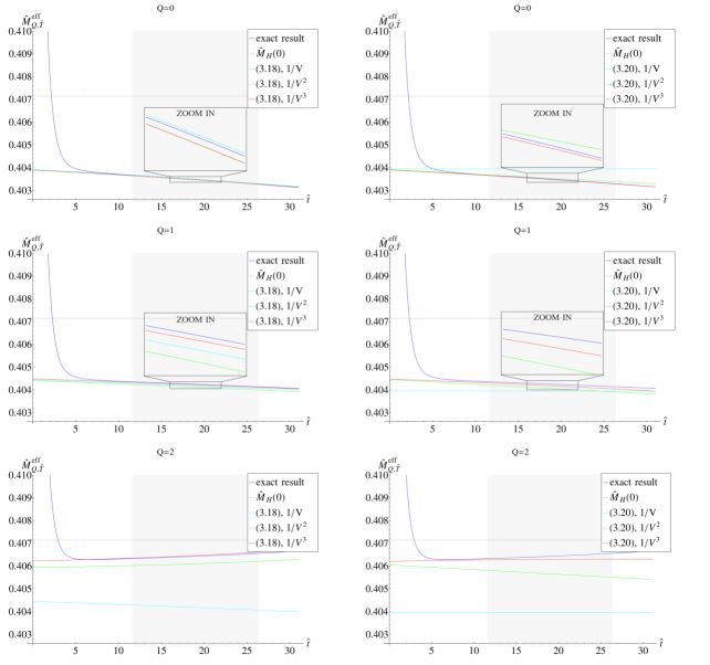
The validity of the shown expansions has been discussed in section 4 and summarized in terms of four conditions, which we check for the quantum mechanical example with parameters , and :
-
•
(C1):
and for , i.e. fulfilled. might need a larger extension. - •
-
•
(C3):
Figure 5.3 shows that (the analog of in QCD) is minimal at , . corresponds to and , i.e. the condition is clearly fulfilled. -
•
(C4):
Figure 5.3 shows that is minimal at , ; therefore, corresponds to . We consider and shade the corresponding safe region in light gray.
Finally can be solved with respect to resulting in . Clearly also this condition is fulfilled.
The effective mass plots shown in Figure 5.5 are consistent with these estimates. There is nearly perfect agreement between the expansions of and the exact results in the gray regions. On the other hand the difference of the effective mass at fixed topology and the mass at unfixed topology (the quantity one is finally interested in) is quite large. This clearly indicates that determining hadron masses from fixed topology simulations with standard methods (e.g. fitting a constant to an effective mass at large temporal separations) might lead to sizable systematic errors, which, however, can be reduced by orders of magnitude, when using the discussed expansions of .
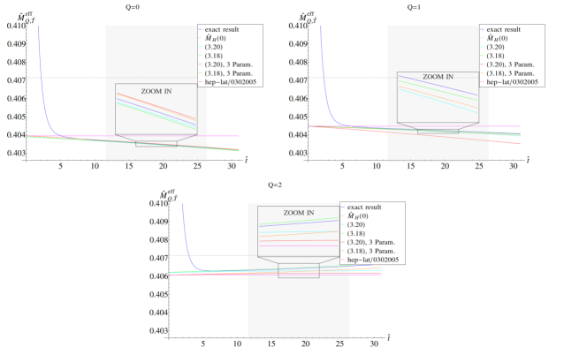
The number of parameters, in particular for the expansions derived up to , i.e. (3.18) and (3.20), is quite large. This could be a problem, when fitting these expressions to lattice results for two-point correlation functions, where statistical accuracy is limited, e.g. for expensive QCD simulations. A possibility to benefit from the higher order expansions at least to some extent, while keeping at the same time the number of fit parameters small, is to use eqs. (3.18) and (3.20) (i.e. expansions up to ), but to set parameters, which are expected to be less important, to zero. In Figure 5.6 we explore this possibility by restricting (3.18) and (3.20) to the parameters , , and , which are the 4 parameters of eq. (3.21), the expansion from the seminal paper [12]. In detail the following curves are shown with the parameters taken from Table 1:
Even though the number of parameters is identical, the “parameter restricted expansions”, in particular (5.21), are significantly closer to the exact result. In practice, when fitting to a correlator from fixed topology QCD simulations with statistical errors, where one is limited in the number of fit parameters, using (5.21) might be the best compromise.
5.3.4 Extracting hadron masses from fixed topology simulations
A straightforward method to determine physical hadron masses (i.e. hadron masses at unfixed topology) from fixed topology simulations based on the expansion (3.21) and (3.22) has been proposed in [12]:
- 1.
-
2.
Determine the hadron mass (the hadron mass at unfixed topology), and by fitting (3.22) to the fixed topology hadron masses obtained in step 1.
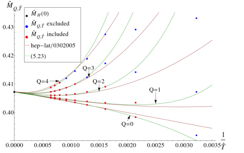
Note, however, that two-point correlation functions at fixed topology do not decay exponentially at large temporal separations (cf. e.g. (3.18)), as their counterparts at unfixed topology do. Therefore, determining a fixed topology and finite volume mass is not clear without ambiguity. One could e.g. define at some temporal separation , where the expansion is a good approximation, i.e. where the conditions (C2) and (C4) from section 4 are fulfilled, using (5.16), i.e.
| (5.23) |
We now follow this strategy to mimic the method to determine a physical hadron mass (i.e. at unfixed topology) from fixed topology computations using the quantum mechanical model. To this end we choose , i.e. a value inside the “safe gray regions” of Figure 5.5 and Figure 5.6. We use the exact result for the effective mass (shown e.g. in Figure 5.4) in (5.23) to generate values for several topological charges and temporal extensions . Then we perform a single fit of either the expansion (3.22) from [12] or our version restricted to three parameters (eq. (5.21)) inserted in (5.23) to these masses , to determine (the hadron mass at unfixed topology), and (the curves in Figure 5.7). Only those masses enter the fit, for which the conditions (C1) (we study both and ) and (C2) from section 4 are fulfilled. Both expansions give rather accurate results for (cf. Table 2, top, column “fitting to ”; the relative errors are below ) and reasonable results for (cf. Table 2, bottom, column “fitting to ”; relative errors of a few percent). Note that the relative errors for both and are smaller, when using the version restricted to three parameters (5.21).
results from fixed topology computations (exact result: )
| fitting to | fitting to correlators | ||||
|---|---|---|---|---|---|
| expansion | result | rel. error | result | rel. error | |
| hep-lat/0302005 | |||||
| (5.21) | |||||
| hep-lat/0302005 | |||||
| (5.21) | |||||
results from fixed topology computations (exact result: )
The drawback of this method is that only fixed topology results at a single value, , enter the final result for the hadron mass at unfixed topology. To exploit the input data and also the derived expansions for the two-point correlation functions at fixed topology more fully, we propose another method:
-
1.
Perform simulations at fixed topology for different topological charges and spacetime volumes . Determine for each simulation.
-
2.
Determine the physical hadron mass by performing a single minimizing fit of the preferred expansions of (in this work we have discussed nine different versions, (3.18) (3.20), (3.21) and (3.22), (5.17), (5.18), (5.19), (5.20), (5.21), (5.22)) with respect to its parameters (cf. section 5.3.3 for a detailed summary of available expansions and their parameters) to the two-point correlation functions obtained in step 1. This input from step 1 is limited to those , and values, for which the conditions (C1), (C2) and (C4) from section 4 are fulfilled.
Note that this method can also be applied when using correlation matrices at fixed topology. Then corresponding expansions, e.g. (3.52) to (3.54), have to fitted simultaneously to all elements of the correlation matrix.
We apply this strategy to the quantum mechanical example using the same and values as before. is limited to and sampled equidistantly. Since our input data is exact777Note that in QCD the exact correlator at fixed topological charge and spacetime volume will be provided by lattice simulations, i.e. has statistical errors., i.e. has no statistical errors, the minimizing fit becomes and ordinary least squares fit. Again we compare the expansion from [12] (eqs. (3.21) and (3.22)) and our version restricted to three parameters (5.21). As before, we find rather accurate results for and (cf. Table 2, columns “fitting to correlators”). Note that the relative errors for both and are smaller, when using the version restricted to three parameters (5.21). The relative errors are also smaller compared to the previously discussed method of “fitting to ”.
6 Conclusions and outlook
In this work we have extended a calculation of the , and dependence of two-point correlation functions at fixed topology from [12]. While in [12] the expansion included all terms of and some of , we have derived the complete result up to . Since in many ensembles of typical nowadays lattice QCD simulations (cf. e.g. [14, 15, 16, 17]), fixed topology corrections of order or even might be sizable, in particular for topological charge , as e.g. demonstrated in Figure 5.6. We have also discussed parity mixing in detail, which appears at fixed topology already at . In particular we have derived corresponding expansions of correlation functions between and operators as well as contributions of opposite parity hadrons to correlation functions between operators of identical parity.
We have applied, discussed and checked our results in the context of a simple model, a quantum mechanical particle on a circle, both in the free case and for a square well potential. We have studied and compared various orders and versions of the expansion of differing in accuracy and in the number of parameters. We also discussed and demonstrated, how to extract a mass at unfixed topology from computations of two-point correlation functions at fixed topology. In practice, e.g. in QCD, where computed two-point correlation functions have limited accuracy, due to statistical errors, one probably needs a expansion of with a rather small number of parameters to be able to perform a stable fit. We recommend to use the expansion (5.21), which seems to be a good compromise:
- •
-
•
At the same time the number of fit parameters is quite small (, and ), the same as for the expansion from [12].
Currently we are applying the equations and methods derived and discussed in this work to simple quantum field theories, e.g. the Schwinger model and pure Yang-Mills theory (cf. also [18, 19, 20, 21, 23] for existing work in this direction). The final goal is, of course, to develop and establish methods to reliably extract hadron masses from QCD simulations at fixed topology.
Appendix A Technical aspects of a quantum mechanical particle on a circle in a square well
A.1 Wave functions
After replacing , Schrödinger’s equation is
| (A.1) |
The wave function with energy in “region 1”, , where , is
| (A.2) |
in “region 2”, , where ,
| (A.3) |
The coefficients , , and have to be chosen such that both the wave function and its derivative are continuous, i.e. that
| (A.4) | ||||
are fulfilled, which is only possible for specific discrete values of . Note that, even after properly normalizing the wave function , its coefficients , , and are only unique up to a phase.
A.2 Probability density to find a particle
The probability density to find a particle with wave function is . In the following it will be shown that .
First note that and fulfill the same Schrödinger equation, which implies
| (A.5) |
where is a non-unique phase.
Now consider region 1, where
| (A.6) |
and
| (A.7) |
Inserting these expressions in (A.5) yields
| (A.8) |
and, consequently,
| (A.9) |
With this relation it is easy to show that the probability density is an even function,
| (A.10) | ||||
Using similar arguments one can show that also in region 2 is an even function.
Acknowledgments
We thank Wolfgang Bietenholz, Krzysztof Cichy, Christopher Czaban, Dennis Dietrich, Gregorio Herdoiza, Karl Jansen and Andreas Wipf for discussions.
We acknowledge support by the Emmy Noether Programme of the DFG (German Research Foundation), grant WA 3000/1-1.
This work was supported in part by the Helmholtz International Center for FAIR within the framework of the LOEWE program launched by the State of Hesse.
References
- [1] A. D. Kennedy, hep-lat/0607038.
- [2] M. Lüscher and S. Schaefer, JHEP 1107, 036 (2011) [arXiv:1105.4749 [hep-lat]].
- [3] S. Schaefer, PoS LATTICE 2012, 001 (2012) [arXiv:1211.5069 [hep-lat]].
- [4] S. Aoki et al. [JLQCD Collaboration], Phys. Rev. D 78, 014508 (2008) [arXiv:0803.3197 [hep-lat]].
- [5] S. Aoki, T. -W. Chiu, G. Cossu, X. Feng, H. Fukaya, S. Hashimoto, T. -H. Hsieh and T. Kaneko et al., PTEP 2012, 01A106 (2012).
- [6] D. Galletly, M. Gurtler, R. Horsley, H. Perlt, P. E. L. Rakow, G. Schierholz, A. Schiller and T. Streuer, Phys. Rev. D 75, 073015 (2007) [hep-lat/0607024].
- [7] H. Fukaya, S. Hashimoto, T. Hirohashi, K. Ogawa and T. Onogi, Phys. Rev. D 73, 014503 (2006) [hep-lat/0510116].
- [8] W. Bietenholz, K. Jansen, K. -I. Nagai, S. Necco, L. Scorzato and S. Shcheredin, JHEP 0603, 017 (2006) [hep-lat/0511016].
- [9] F. Bruckmann, F. Gruber, K. Jansen, M. Marinkovic, C. Urbach and M. Wagner, Eur. Phys. J. A 43, 303 (2010) [arXiv:0905.2849 [hep-lat]].
- [10] K. Cichy, G. Herdoiza and K. Jansen, Nucl. Phys. B 847, 179 (2011) [arXiv:1012.4412 [hep-lat]].
- [11] K. Cichy, V. Drach, E. Garcia-Ramos, G. Herdoiza and K. Jansen, Nucl. Phys. B 869, 131 (2013) [arXiv:1211.1605 [hep-lat]].
- [12] R. Brower, S. Chandrasekharan, J. W. Negele and U. J. Wiese, Phys. Lett. B 560, 64 (2003) [hep-lat/0302005].
- [13] S. Aoki, H. Fukaya, S. Hashimoto and T. Onogi, Phys. Rev. D 76, 054508 (2007) [arXiv:0707.0396 [hep-lat]].
- [14] S. Aoki et al. [JLQCD and TWQCD Collaborations], Phys. Lett. B 665, 294 (2008) [arXiv:0710.1130 [hep-lat]].
- [15] T. W. Chiu, T. H. Hsieh and Y. Y. Mao, Phys. Lett. B 702, 131 (2011) [arXiv:1105.4414 [hep-lat]].
- [16] K. Cichy et al. [ETM Collaboration], JHEP 1402, 119 (2014) [arXiv:1312.5161 [hep-lat]].
- [17] R. C. Brower et al. [LSD Collaboration], arXiv:1403.2761 [hep-lat].
- [18] W. Bietenholz, I. Hip, S. Shcheredin and J. Volkholz, Eur. Phys. J. C 72, 1938 (2012) [arXiv:1109.2649 [hep-lat]].
- [19] W. Bietenholz and I. Hip, J. Phys. Conf. Ser. 378, 012041 (2012) [arXiv:1201.6335 [hep-lat]].
- [20] C. Czaban and M. Wagner, arXiv:1310.5258 [hep-lat].
- [21] I. Bautista, W. Bietenholz, U. Gerber, C. P. Hofmann, Héc. Mejía-Díaz and L. Prado, arXiv:1402.2668 [hep-lat].
- [22] A. Dromard and M. Wagner, arXiv:1309.2483 [hep-lat].
- [23] C. Czaban, A. Dromard and M. Wagner, arXiv:1404.3597 [hep-lat].
- [24] S. R. Coleman, Subnucl. Ser. 15, 805 (1979).
- [25] C. Bonati, M. D’Elia, H. Panagopoulos and E. Vicari, Phys. Rev. Lett. 110, 252003 (2013) [arXiv:1301.7640 [hep-lat]].
- [26] J. Weber, S. Diehl, T. Kuske and M. Wagner, arXiv:1310.1760 [hep-lat].
- [27] K. Jansen et al. [ETM Collaboration], JHEP 0812, 058 (2008) [arXiv:0810.1843 [hep-lat]].
- [28] C. Michael, A. Shindler and M. Wagner [ETM Collaboration], JHEP 1008, 009 (2010) [arXiv:1004.4235 [hep-lat]].
- [29] R. Baron et al. [ETM Collaboration], Comput. Phys. Commun. 182, 299 (2011) [arXiv:1005.2042 [hep-lat]].
- [30] M. Wagner and C. Wiese [ETM Collaboration], JHEP 1107, 016 (2011) [arXiv:1104.4921 [hep-lat]].
- [31] M. Kalinowski and M. Wagner [ETM Collaboration], PoS ConfinementX , 303 (2012) [arXiv:1212.0403 [hep-lat]].
- [32] M. Kalinowski and M. Wagner [ETM Collaboration], Acta Phys. Polon. Supp. 6, no. 3, 991 (2013) [arXiv:1304.7974 [hep-lat]].
- [33] M. Kalinowski and M. Wagner [ETM Collaboration], PoS LATTICE 2013, 241 (2013) [arXiv:1310.5513 [hep-lat]].