Stability and instability of expanding solutions to the Lorentzian constant-positive-mean-curvature flow

Abstract.

We study constant mean curvature Lorentzian hypersurfaces of $\mathbb{R}^{1,d+1}$ from the point of view of its Cauchy problem. We completely classify the spherically symmetric solutions, which include among them a manifold isometric to the de Sitter space of general relativity. We show that the spherically symmetric solutions exhibit one of three (future) asymptotic behaviours: (i) finite time collapse (ii) convergence to a time-like cylinder isometric to some $\mathbb{R}\times\mathbb{S}^{d}$ and (iii) infinite expansion to the future converging asymptotically to a time translation of the de Sitter solution. For class (iii) we examine the future stability properties of the solutions under arbitrary (not necessarily spherically symmetric) perturbations. We show that the usual notions of asymptotic stability and modulational stability cannot apply, and connect this to the presence of cosmological horizons in these class (iii) solutions. We can nevertheless show the global existence and future stability for small perturbations of class (iii) solutions under a notion of stability that naturally takes into account the presence of cosmological horizons. The proof is based on the vector field method, but requires additional geometric insight. In particular we introduce two new tools: an inverse-Gauss-map gauge to deal with the problem of cosmological horizon and a quasilinear generalisation of Brendle’s Bel-Robinson tensor to obtain natural energy quantities.

1. Introduction

In this paper we study Lorentzian (i.e. time-like) hypersurfaces $M\subset\mathbb{R}^{1,d+1}$ of $d+2$ dimensional Minkowski spaces with constant, positive mean curvature (“$M$ is $\mathrm{C}_{+}\mathrm{MC}$”). The limiting case where $M$ has everywhere vanishing mean curvature (“$M$ is $\mathrm{C}_{0}\mathrm{MC}$”) is actively studied under names such as relativistic membranes and extremal or time-like minimal/maximal hypersurfaces. Mathematically they give rise to natural classes of quasilinear wave equations with clear geometric interpretation, and serve as a testing ground for development of techniques in geometric analysis and in the study of nonlinear waves on curved backgrounds; some recent successes can be found in [DKSW13, NT13, Lin04, Bre02]. On the other hand, manifolds which are $\mathrm{C}_{0}\mathrm{MC}$ give one plausible description of a classical (as opposed to quantum), relativistic, extended test object moving freely in space [AC79a]. Understanding such objects seems to be a first step toward the quantization of extended relativistic objects (see [Hop13] for a recent topical review of the physical perspective).

If $\mathrm{C}_{0}\mathrm{MC}$ manifolds are “freely evolving”, then $\mathrm{C}_{+}\mathrm{MC}$ manifolds are those subject to a “constant normal force”. The analogy is clearest when we start with dimension $d=0$. The ambient space-time is then a $2$-dimensional Lorentzian manifold, and our manifold $M$ is simply a curve. By assumption $M$ is taken to be time-like, and so we interpret it as the world-line of a particle. Taking an arc-length (i.e. proper time) parametrisation, the mean curvature of $M$ is nothing more than the acceleration of this particle! Hence in the $d=0$ case, the $\mathrm{C}_{0}\mathrm{MC}$ manifolds are geodesics, and the $\mathrm{C}_{+}\mathrm{MC}$ manifolds are those subject to a constant force, once we appeal to Newton’s second law. (See also the discussion in [AC79a].)

(It is interesting to note that one can alternatively characterise geodesics in a pseudo-Riemannian manifold as the image of a harmonic map from $\mathbb{R}$. Swapping the source space to a higher-dimensional manifold gives another possible interpretation of what it means to describe a freely evolving, classical, relativistic, extended test object.)

Just as the equations describing a Riemannian hypersurface of prescribed mean curvature have an elliptic nature, the equations describing our Lorentzian hypersurfaces are hyperbolic partial differential equations, with a locally well-posed initial value problem. The easiest way to see this is to fix a point $x\in M$ and consider $M$, locally in a neighbourhood of $x$, as a graph over the tangent plane $\Pi_{x}$ to $M$. Letting $\phi$ be the height of the graph (in the direction of the Minkowski normal direction to $\Pi_{x}$), the mean curvature (see Appendix A.2 for a quick review) of $M$ is given by

(1.1) $$\text{mean curvature}=\frac{\partial}{\partial y_{i}}\left(\frac{m^{ij}\frac{\partial}{\partial y_{j}}\phi}{\sqrt{1+m^{ij}\partial_{i}\phi\partial_{j}\phi}}\right)$$

where $\{y_{0},\dots,y_{d}\}$ is a flat (Minkowski) coordinate system for the hyperplane $\Pi_{x}$ and $m^{ij}$ is the induced Minkowski metric with signature $(-+\cdots+)$. That $M$ remains time-like is captured in the condition $1+m^{ij}\partial_{i}\phi\partial_{j}\phi>0$. Cast in this form it is evident that $\mathrm{C}_{+}\mathrm{MC}$ and $\mathrm{C}_{0}\mathrm{MC}$ manifolds can be locally described by quasilinear wave equations, which classically admit well-posed initial value problems [CH62, HKM76, Kla80]. Taking advantage of the finite speed of propagation for such equations, these local descriptions can be glued together (a technique common in geometric wave equations and mathematical relativity, see e.g. [FB52, Rin09, KM95]) to get the desired local existence of evolution.

Remark 1.1.

More precisely, the Cauchy problem of the constant mean curvature flow can be phrased as following. Let $\Sigma$ be a $d$–dimensional smooth manifold, and $H$ the value of the prescribed mean curvature. Our initial data is $\Upsilon_{0}:\Sigma\to\mathbb{R}^{1,d+1}$ a (sufficiently regular) embedding such that $\Upsilon_{0}(\Sigma)$ is a space-like submanifold, together with $\Upsilon_{1}:\Sigma\to\mathbb{R}^{1,d+1}$ a family of future-directed time-like vectors. A solution to the Cauchy problem is an embedding $\Upsilon:\mathbb{R}\times\Sigma\to\mathbb{R}^{1,d+1}$ satisfying $\Upsilon(\mathbb{R}\times\Sigma)$ has the constant mean curvature $H$, such that $\Upsilon(0,\mathord{\bullet})=\Upsilon_{0}(\mathord{\bullet})$ and that the image of $\mathrm{d}{\Upsilon}(0,\mathord{\bullet})$ is spanned by the image of $\mathrm{d}{\Upsilon_{0}}(\mathord{\bullet})$ and $\Upsilon_{1}(\mathord{\bullet})$. Note that phrased in this way there is considerable gauge freedom in the diffeomorphism $\Upsilon$ due to diffeomorphism invariance. To get a well-posed problem one would need to fix a gauge or coordinate system. When $\Upsilon_{0}$ takes value in $\{0\}\times\mathbb{R}^{d+1}\subset\mathbb{R}^{1,d+1}$ a convenient gauge is to require that $\Upsilon(t,\mathord{\bullet})\in\{t\}\times\mathbb{R}^{d+1}$ and that $\partial_{t}\Upsilon(t,\mathord{\bullet})$ be orthogonal to $\Upsilon(t,\Sigma)$. It is relatively simple to convert between a solution described in this gauge with the local solution defined by solving (1.1).

For obtaining global estimates in the case where $\Sigma$ is a $d$–dimensional (topological) sphere, and the initial data $\Upsilon_{0,1}$ are “sufficiently small”, it turns out a more convenient gauge choice is what we will call the inverse-Gauss-map gauge, and which we will discuss in Section 4.

When facing an evolution equation with well-posed local dynamics, it is natural to ask “for which classes of initial data do we have global existence of solutions?” When furthermore certain explicit solutions are known, it is also natural to ask “are the behaviours exhibited by those explicit solutions stable?” These two questions drive the analysis of the current paper.

1.1. Some known results in the $\mathrm{C}_{0}\mathrm{MC}$ case

To give examples of the type of answers that one looks for in regards to the two questions above, let us briefly review the recent progress concerning the case of $\mathrm{C}_{0}\mathrm{MC}$ manifolds.

The first results concerning global stability are that for the “trivial solution” of the $\mathrm{C}_{0}\mathrm{MC}$ equations. One easily sees that the Minkowski space $\mathbb{R}^{1,d}$ embeds in $\mathbb{R}^{1,d+1}$ as a hyperplane, and this embedding is totally geodesic, and hence has vanishing mean curvature. Brendle ([Bre02] for $d\geq 3$) and Lindblad ([Lin04] for $d=2$) were able to show that starting with initial data “sufficiently close” (in a Sobolev sense) to one of these time-like hyperplanes, the solution to the $\mathrm{C}_{0}\mathrm{MC}$ equations exist for all time and converges asymptotically in time back to said hyperplane.

As the solution is a perturbation of a hyperplane, the manifold $M$ in this case can be globally represented as a graph. The results and Brendle and Lindblad can thus be understood, via (1.1), as a statement about global well-posedness and scattering for a quasilinear wave equation on $\mathbb{R}^{1,d}$, and in fact can be deduced from earlier works of Christodoulou [Chr86] and Klainerman [Kla86]. The decay that drives the asymptotic convergence then takes its origins in the linear decay of waves on Minkowski space with $d\geq 2$, and the crucial observation that allows the nonlinearity to be controlled by the linear decay is that (1.1) obeys both the quadratic [Chr86, Kla86] and, in Lindblad’s case, the cubic [Ali01a, Ali01b] null conditions.

There are, of course, other known explicit global solutions to the $\mathrm{C}_{0}\mathrm{MC}$ equations. In fact, if one starts with any complete minimal hypersurface in $\mathbb{R}^{d+1}$, extending it trivially in the time direction leads to a geodesically complete $\mathrm{C}_{0}\mathrm{MC}$ manifold $M$. One can then ask whether the same stability property enjoyed by the hyperplane shown by Brendle and Lindblad (global existence for perturbed initial data, asymptotic decay of the perturbation) is also shared by such $M$. Exactly this question was studied recently by the author, together with R. Donninger, J. Krieger, and J. Szeftel, for $M$ being the stationary solution generated by the catenoid, with $d=2$ [DKSW13]. The catenoid is variationally unstable as a minimal surface [FCS80], a fact leading directly to linear instability of the stationary catenoid solution under the $\mathrm{C}_{0}\mathrm{MC}$ flow. Nevertheless, in [DKSW13] the authors were able to construct a centre manifold for the evolution: under some symmetry assumptions (which in particular allows the authors to avoid some difficulty having to do with the trapping of null geodesics) they were able to show the existence of a co-dimension 1 set of small perturbations which evolve into solutions that converge asymptotically back to the catenoid. The main decay mechanism here is, again, the dispersive decay of solutions to the linear wave equation (on a now curved background, and with a short-range potential); here they crucially exploited the catenoid’s nature as an asymptotically flat manifold.

On the other hand certain blow-up results are available. It is expected that for $M$ arising from initial data that is a compact manifold, one should have finite time singularity formation under the $\mathrm{C}_{0}\mathrm{MC}$ equations. This is motivated in part by the non-existence of compact minimal hypersurfaces in $\mathbb{R}^{d+1}$, which implies there are no stationary solutions to the $\mathrm{C}_{0}\mathrm{MC}$ equations with compact spatial cross-section. The singularity formation can also be easily verified in the spherically symmetric case. Here the manifold can be described as the set $\{r=f(t)\}$ where $f$ solves the nonlinear ordinary differential equation (see also Section 2 below)

(1.2) $$0=ff^{\prime\prime}+d[1-(f^{\prime})^{2}].$$

That the manifold is time-like requires $|f^{\prime}|<1$, and by assumption $f>0$ (it is the value of the radial coordinate). From convexity one can easily see the finite time collapse of any initial data. (For $d=1,2$ the equation can be explicitly solved in terms of trigonometric and Jacobi elliptic functions respectively.) Outside of spherical symmetry, the recent work of Nguyen and Tian [NT13] verified singularity formation in dimension $d=1$ for initial data being a closed curve, and provided detailed information about the behaviour of the solution at the singular point.

1.2. Positive mean curvature

An immediate difference one notices when studying the $\mathrm{C}_{+}\mathrm{MC}$ case is that there exist global-in-time solutions with compact spatial cross sections. In fact, as the sphere $\mathbb{S}^{d}\subset\mathbb{R}^{d+1}$ is a constant positive mean curvature hypersurface, its trivial extension in time gives a stationary $\mathrm{C}_{+}\mathrm{MC}$ manifold; physically one may think of this as a soap bubble supported by a pressure differential. As we will discuss in Section 2 below in the context of spherical symmetry and time-symmetric initial data, for a fixed value of the mean curvature, this static solution forms a barrier between solutions which collapses in finite time (both in the future and in the past) and solutions which expand indefinitely. This immediately implies the instability of this stationary solution (which is isometric to the Einstein cylinder) under small perturbations, which then leads to an interesting open question in the direction of [DKSW13]:

Question 1.

Does there exist some non-trivial set of initial perturbations of the data generating $\mathbb{R}\times\mathbb{S}^{d}$ on which the $\mathrm{C}_{+}\mathrm{MC}$ flow (with mean curvature $d$) is orbitally stable?

A few remarks are in order. Firstly, the question is stated in terms of orbital stability instead of asymptotic stability as the latter would essentially require proving certain small data solutions to a quasilinear wave equation on the Einstein cylinder decay in time. This seems highly unlikely to the author as even for the linear wave equation on the Einstein cylinder one has no dispersive decay (there are finite energy mode solutions whose amplitudes are constant in time). Secondly, once we allow ourselves to consider solutions which remain bounded asymptotically, there are obvious initial perturbations, which correspond to the translation symmetries of $\mathbb{R}^{d+1}$, leading to orbital stability; hence the requirement that the initial perturbation is non-trivial.

We will not address Question 1 in this paper beyond the spherically symmetric case; see Theorem 2.21. Instead, the main focus is the following, slightly easier problem.

Question 2.

Are the spherically symmetric expanding solutions “outside” the “Einstein cylinder” stable under the $\mathrm{C}_{+}\mathrm{MC}$ flow in any sense?

That this question may be more tractable comes from the expansion of the background solution. That the expansion of space-time can drive the decay of solutions to wave equations, even when the spatial topology is compact, is a well-studied phenomenon from the study of space-times with positive cosmological constant in general relativity. In some cases the decay given by this expansion can be seen as stronger and giving rise to better estimates, compared to the dispersion on a flat space-time. For the linear wave equation, for example, the accelerated expansion of the space-time leads to exponential (in proper time) decay of solutions to a constant (see, e.g. [MSBV14] and references therein); dispersion on a flat space-time only gives polynomial decay. For a nonlinear example one may consider Friedrich’s proof of the stability of de Sitter space [Fri86] compared to the Christodoulou-Klainerman theorem on stability of Minkowski space [CK93].

It is however easy to see that the answer to Question 2 must be in the negative if one studies the perturbed solution $M$ as a graph in the normal bundle over the spherically symmetric expanding background. A first class of unstable perturbations are easily understood: again we make use of the symmetries of the ambient space-time. Isometries of $\mathbb{R}^{1,d+1}$ send $\mathrm{C}_{+}\mathrm{MC}$ manifolds to other $\mathrm{C}_{+}\mathrm{MC}$ manifolds; the spatial and temporal translations in particular preserves none of the spherically symmetric expanding solutions. As we shall see in Section 3.2, the corresponding perturbations grow exponentially in proper time. A second class of perturbations correspond to the purely radial perturbations. From the analysis of the corresponding ODE system in Section 2, we will also see that these give rise to also exponentially growing perturbations.

Remark 1.2.

It turns out that the rate of growth depends on how one measures time and how one measures the deviation of a solution from the spherically symmetric expanding background. For the former it is convenient to measure with respect to a time function that is “proper” (by which we mean has unit length) relative to the induced Lorentzian geometry of the spherically symmetric expanding background. The latter is more complicated. If one treats the solution as a graph in the normal bundle of the background, then we indeed have linear instability leading to exponential growth (and in particular neither asymptotic nor orbital stability holds). In terms of the formulation given in Section 2 where the solutions are described as graphs $r=f(t)$, the orbital stability of solutions is an easy corollary of the analyses leading up to Theorem 2.22. In Section 9.1 we will also see how one can interpret the spherically symmetric expanding solutions as orbitally stable under general perturbations; this, however, will be a direct consequence of the our more detailed control on the asymptotic behaviour of solutions.

In order to deal with these unstable perturbations, a commonly used technique is that of modulation theory, originally introduced for proving orbital (instead of asymptotic) stability of certain stationary solutions of semilinear equations [Wei85, Wei86]. A key feature to this theory is to identify a finite dimensional subspace (the modulation space) of the solution space which captures the instability (in the asymptotic sense) of the (linearised) evolution. The partial differential equation then is decomposed as a coupled system of ordinary differential equations (the modulation equations) describing the trajectory (of the projection) on the modulation space along with a partial differential equation describing the dynamics transverse to the modulation space. The choice of the modulation space and modulation equations are so that the remaining PDE enjoys better stability or compactness properties, rendering the problem more tractable. In many (semilinear) cases the modulation equations can be tracked “in the large”, leading to results on orbital stability or stable blow-up dynamics (e.g. [MRS10, RR12]). For quasilinear equations, the dependence of the linearised operator on the background solution makes the procedure more delicate; but if one restricts attention to showing the existence of a centre manifold for the evolution, the basic method of Lyapunov and Perron can be viewed as a “baby” version of modulation theory, from which some success can be obtained (for example [DKSW13]).

If one were to try to adapt the idea of modulation theory (or at the very least, the Lyapunov-Perron method) naïvely to the $\mathrm{C}_{+}\mathrm{MC}$ setting to study the stability of spherically symmetric expanding solutions, one runs into an obstacle tied to the background geometry. As is well-known in the literature in mathematical relativity, a feature of expanding solutions such as the de Sitter geometry or the Friedmann-Lemaître-Robertson-Walker (FLRW) geometry is the presence of cosmological horizons. Roughly speaking, from the intrinsic point of view the space-time may be expanding faster than the speed of light, leading to regions which asymptotically cannot communicate with each other. (This will be explained in more detail in Section 3.) The net effect of these cosmological horizons is that, asymptotically, one needs to keep track of an infinite dimensional modulation space, which effectively obviates the advantages usually proffered by the use of modulation theory.

Our resolution of this conundrum is through a geometrically motivated replacement of modulation theory, which in practice is implemented through a good gauge choice (see Section 4). The rough idea is the following: an analysis of the spherically symmetric expanding solutions shows that they all share the same asymptotic profile. This suggests that at the derivative level the perturbations should “converge to zero”. One should then try to formulate the equation “at the level of the first derivative”. (Note that the perturbation equations for the solution described as a graph over the perturbed background have a scalar dependence on the solution itself, so formulating the equation for the derivatives is not as simple as just commuting the equation with a differential operator.)

An imperfect analogy can be drawn with the various proofs of the stability of Minkowski space. In harmonic coordinates, the vacuum Einstein equations can be written as a quasilinear wave equation for the components of the metric itself. This equation however does not satisfy the classical null condition and it is not until the recent work of Lindblad and Rodnianski [LR10, LR05] that the global behaviour of small-data solutions is understood in terms of the so-called weak null condition. Furthermore, asymptotically there is a certain loss of control for solutions to equations satisfying the weak null condition compared to those to equations satisfying the classical null condition [Ali03, Lin08], a phenomenon having to do with the fact that the background Minkowskian geometry is a poor approximation of the true dynamical null geometry of the solution. Morally speaking this corresponds to the approach studying the $\mathrm{C}_{+}\mathrm{MC}$ problem as a quasilinear equation for the height function of a graph over a background $\mathrm{C}_{+}\mathrm{MC}$ manifold. Our approach, then, is more similar to the proof of Christodoulou and Klainerman [CK93]. There the authors studied an system of associated equations at the level of the second derivatives of the unknown metric (the Weyl curvature), with one family of equations (the Bianchi identities) arising from an integrability constraint (morally that the curvature is the “derivative of something else”), and another (the dual Bianchi identities) a consequence of the original vacuum Einstein equations (note that the vacuum Einstein equations is “lower order” than the dual Bianchi identities). One exploits the dispersive nature of this system of equations (obtained by considering the true dynamical null geometry of the solution) to gain decay estimates, which one can then integrate (null structure equations) to obtain control on the first derivatives of the metric (Ricci rotation coefficients). As will be discussed in Section 4, we will study for the $\mathrm{C}_{+}\mathrm{MC}$ system also an associated system of equations at “higher order” than the statement of constant mean curvature, consisting of an integrability constraint and an equation derived as a consequence of constant mean curvature. This will allow us to directly prove the decay on the level of derivatives without worrying about the possible exponential growth of the height function itself.

At this point we should mention that similar results (exponential growth of the unknown together with decay of derivatives) have also been obtained recently in the context of nonlinear stability of spatially homogeneous solutions to coupled systems of Einstein’s equation with positive cosmological constant with various matter fields [Rin08, RS13, Spe12, Spe13, HS13]. The positive cosmological constant drives an accelerated expansion and leads naturally to discussions similar to Question 2. A typical feature of the results mentioned here is that the control obtained for the fundamental unknown, which let us call $u$, takes the form

$$\left\lVert e^{-t}u(t,\cdot)-u_{0}(\cdot)\right\rVert_{\infty}\lesssim e^{-t}$$

while

$$\left\lVert u_{0}\right\rVert_{\infty}\approx\epsilon$$

where $\epsilon$ is the size of the initial perturbation, while for higher derivatives of $u$ one gets improved decay. In particular, for the unknown $u$ itself, one cannot prove that it decays to zero, even after renormalisation; one can only expect (renormalisable) exponential growth. This freezing-in of the initial perturbation seems to be a stable feature of stability problems for background with accelerated expansion. Compare to this our geometrical approach provides a small gain: we are in fact able to extract quite precisely the asymptotic behaviour of our perturbed solutions (see next section).

We remark here also that the methods employed in [Rin08, RS13, Spe12, Spe13, HS13] study directly the equations at the level of the metric (similar to [LR05] and comparable to the case of studying the height function of the graphical description in our problem), and requires carefully keeping track the structure of the equation to verify that the exponential growth of the unknown itself will not cause problems. In comparison our geometric approach allows us to be much more schematic when considering the structure of the equations — this is attested in the relative simplicity of the proof of Theorem 8.1 below. Unfortunately it is not clear to the author whether a similar approach is available to treat the problems in general relativity.

1.3. Main results and outline of paper

We start with some remarks. First, we will use throughout the Japanese bracket notation $\left\langle x\right\rangle\overset{\mbox{\tiny{def}}}{=}\sqrt{1+x^{2}}$ for $x\in\mathbb{R}$. Secondly, we give a quick review of pseudo-Riemannian geometry in the Appendix, which includes setting of the convention for the definition of the mean curvature (in our convention the unit sphere $\mathbb{S}^{d}\subset\mathbb{R}^{d+1}$ has positive mean curvature $d$). Thirdly, examining the behaviour of the mean curvature under scaling transformations (see Appendix A.2 and (A.5b)), we see that when studying the $\mathrm{C}_{+}\mathrm{MC}$ problem, we can assume without loss of generality that the mean curvature scalar is fixed to be $(d+1)$.

In Section 2, we study the $\mathrm{C}_{+}\mathrm{MC}$ problem in spherical symmetry. The equations of motion reduce to a single second order ordinary differential equation, and we completely classify its asymptotic behaviour (including the blow-up cases), first qualitatively in Section 2.1 and then quantitatively in Section 2.2. As we have already seen above, symmetries of the ambient space can generate instabilities for the associated equations of motion; a fact we will recover from our analysis. However, our asymptotic profile also implies that this is the only instability in the spherical symmetric case, and we have indeed a modulational stability result. To illustrate, we give here a rough version of Theorem 2.22.

Theorem 1.3.

Let $M=\left\{\;(t,x)\in\mathbb{R}_{+}\times\mathbb{R}^{d+1}\;\middle|\;\left\lvert x\right\rvert=f(t)\;\right\}$ denote a spherically symmetric $\mathrm{C}_{+}\mathrm{MC}$ manifold, such that the defining function $f(t):\mathbb{R}_{+}\to\mathbb{R}_{+}$ satisfies $\lim_{t\to\infty}f(t)=\infty$. Then $M$ as an individual solution is unstable under small perturbations. However, the family of all time translations of $M$ is future asymptotically stable.

The natural question to ask after the previous theorem is whether it extends to the case without spherical symmetry. In Section 3 we show that the answer is no, by exploiting the finite speed of propagation properties of hyperbolic partial differential equations, and the presence of so-called “cosmological horizons” on expanding space-times such as de Sitter space $\mathcal{M}_{\mathrm{dS}}$ (see Appendix A.3 for the definition). The main results of this section are Theorems 3.5 and 3.6. The first theorem applies to the linearised equation around $\mathcal{M}_{\mathrm{dS}}$, where the solution is treated as a graph over the normal bundle of $\mathcal{M}_{\mathrm{dS}}$: it indicates that the linearised equation has an infinite dimensional set of unstable directions, making naive applications of modulation theory unsuitable. The second theorem shows that the (finite dimensional) family generated by the application of the Poincaré group to $\mathcal{M}_{\mathrm{dS}}$ cannot exhaust all possible asymptotic structures, in stark contrast to the spherically symmetric case.

The remaining sections are devoted to proving that, in spite of the results obtained in Section 3, one can still have a positive answer to Question 2 if one refines the notion of “stability”. (We remark here that while the Sections 2 and 3 have some independent interest and lays the motivation and intuition for the rest of the paper, the material presented in the remaining sections are essentially logically independent.) Returning to the issue of cosmological horizons, we see that it forces an asymptotic decoupling of disjoint spatial regions of the solution. Thus one should expect that, in order to apply some sort of modulation theory, the modulation parameter should no longer be just a running function of time. Instead, it should be given by a function defined over the entire space-time: this nicely dovetails with the intuition that the modulation space is infinite dimensional. The actual implementation of this idea, however, is geometrical: we find a mapping from our perturbed manifold to the standard $\mathcal{M}_{\mathrm{dS}}$ such that certain geometric quantities (including the difference of the induced metrics and the difference of induced second fundamental forms and their derivatives) decay asymptotically. We may interpret our final result (Theorem 9.1) as

Theorem 1.4.

Let $M$ be the (future) $\mathrm{C}_{+}\mathrm{MC}$ manifold generated by a small perturbation of the initial data for a spherically symmetric, future expanding solution described in Section 2 (which includes, in particular, the $\mathcal{M}_{\mathrm{dS}}$ solution). Then as long as the initial perturbation is sufficiently small, we have that

• $M$ is future global;

• $M$ converges in time, spatially locally, to a (space-time) translation of the original expanding solution. By spatially locally one should think a notion such as “along tubular neighbourhoods ‘of fixed spatial size $\epsilon\ll 1$’ of time-like curves”.

In order to obtain the above results, we introduce two new tools, which, to the specialists, would be the main contribution of this paper. The first, as already mentioned, is the inverse-Gauss-map gauge, our geometric replacement for modulation theory. This is developed in Section 4. Under the inverse-Gauss-map gauge, the equations of motions reduce to a relatively simple form (4.18) which is a quasilinear divergence-curl system. To establish the suitable a priori energy estimates for demonstrating decay, we first refine Brendle’s Bel-Robinson tensor [Bre02] in Section 5 to a very general setting in order to apply to our quasilinear situation. This allows us to prove $L^{2}$-based energy estimates in Section 7.1; these estimates are somewhat unintuitively weighted in time (the unweighted $L^{2}$ norms are allowed to grow exponentially in proper time). The favourable geometry of $\mathcal{M}_{\mathrm{dS}}$ allows us to dwarf this growth by the exponential growth of the spatial volume, which, via a Sobolev embedding, gives that the $L^{\infty}$ norm will in fact decay exponentially (in proper time), assuming boundedness of the weighted $L^{2}$ energy. Small data global existence and asymptotic stability then follows by a standard bootstrap argument.

In writing up this paper, concision is sacrificed for motivation and for a desire for the manuscript to be reasonably self-contained. The author wishes the readers grant him this indulgence.

1.4. Acknowledgements

This paper has its genesis in a question posed to the author by Lars Andersson at the 2014 OXPDE workshop in Nonlinear Wave Equations and General Relativity; as such the author must thank Lars for the interesting question, and also OXPDE, especially Gui-Qiang Chen and Qian Wang, for their hospitality. The research for this paper can thus be said to have its seeds sown at Oxford; the author is otherwise supported by the Swiss National Science Foundation through a grant to Joachim Krieger, who has on many occasions also lent the author his sympathetic ear. The author would also like to thank Joules Nahas for several profitable discussions; Jared Speck for clarifying some details of his work on the stability of expanding FLRW solutions; and Demetrios Christodoulou for some insightful comments on the manuscript.

2. Rotationally symmetric solutions

Under rotational symmetry, the equation for constant mean curvature reduces to an ordinary differential equation in the extrinsic time variable $t$: let $r$ be the radial coordinate, the inward unit normal to the rotationally symmetric surface given by the graph of $r=f(t)$ is

$$\vec{n}=-\frac{1}{\sqrt{1-(f^{\prime})^{2}}}(\partial_{r}+(f^{\prime})\partial_{t}).$$

A direct computation yields that the nonlinear ODE for constant mean curvature $c$ is

(2.1) $$[1-(f^{\prime})^{2}]d+ff^{\prime\prime}=c[1-(f^{\prime})^{2}]^{\frac{3}{2}}f,$$

as indicated before, by rescaling we can fix $c=d+1$ for convenience. We can equivalently write (2.1), with the choice of $c$ fixed, as

(2.2) $$\left(\frac{f^{\prime}}{\sqrt{1-(f^{\prime})^{2}}}\right)^{\prime}=(d+1)-\frac{d}{f\sqrt{1-(f^{\prime})^{2}}}.$$

The equation (2.1) admits two explicit solutions. The pseudo-sphere $\mathcal{M}_{\mathrm{dS}}=\mathbb{S}^{1,d+1,1}$ as described in Appendix A.3 corresponds to the solution $f(t)=\left\langle t\right\rangle$. Another explicit solution is given by the cylinder $f(t)\equiv\frac{d}{d+1}$. Note that as (2.1) is autonomous, time translations of solutions are also solutions.

In this section we will analyse the ODE (2.1) and describe the asymptotic behaviours of the solutions. Observe that from the fundamental theorem of existence and uniqueness of ordinary differential equations, if $f(t_{0})\neq 0$ and $\left\lvert f^{\prime}(t_{0})\right\rvert<1$, the equation (2.1) has an unique local solution also satisfying $f\neq 0$ and $\left\lvert f^{\prime}\right\rvert<1$. These two conditions are geometric in nature: when $f=0$ the solution manifold $\{r=f(t)\}$ collapses to a point and fails to be regular, while when $\left\lvert f^{\prime}\right\rvert=1$ the induced pseudo-Riemannian structure on the solution manifold $\{r=f(t)\}$ becomes degenerate. We first prove a blow-up criterion.

Proposition 2.1.

Let $\left\lvert t_{1}\right\rvert,\left\lvert t_{2}\right\rvert<\infty$, and let $f:(t_{1},t_{2})\to\mathbb{R}_{+}$ be a $C^{2}$ solution of (2.1). If $\sup_{(t_{1},t_{2})}\left\lvert\log f\right\rvert<\infty$, and $\left\lvert f^{\prime}(t_{0})\right\rvert<1$ for some $t_{0}\in(t_{1},t_{2})$, then $\sup_{(t_{1},t_{2})}\left\lvert f^{\prime}\right\rvert<1$.

Proof.

Consider the quantity $u=1-(f^{\prime})^{2}$. A direct computation from (2.1) gives

(2.3) $$(\log u)^{\prime}=\frac{u^{\prime}}{u}=2\frac{f^{\prime}}{f}\left[d-(d+1)fu^{\frac{1}{2}}\right].$$

Observe that $u>0\implies\left\lvert f^{\prime}\right\rvert<1$, and that by construction $u\leq 1$. Thus the right-hand side of (2.3) is bounded whenever $u>0$ and $\log f$ is bounded. Let $U$ be the connected component containing $t_{0}$ of the open subset $\left\{\;t\in(t_{1},t_{2})\;\middle|\;u>0\;\right\}$. Integrating (2.3) from $t_{0}$, using the boundedness of $t_{1},t_{2}$, gives that $\sup_{U}\left\lvert\log u\right\rvert<\infty$, and hence $U$ is closed. Therefore $U=(t_{1},t_{2})$ and $\sup_{(t_{1},t_{2})}\left\lvert f^{\prime}\right\rvert<1$. ∎

The implied bound on $f^{\prime}$ in Proposition 2.1 also shows that starting from initial data $f(t_{0})>0$ and $\left\lvert f^{\prime}(t_{0})\right\rvert<1$, the solution $f$ cannot blow-up to $\infty$ in finite time. Hence we have the continuation criterion

Corollary 2.2.

With initial data $f(t_{0})\in\mathbb{R}_{+}$ and $f^{\prime}(t_{0})\in(-1,1)$, the solution can be extended as long as $f$ is bounded away from $0$.

2.1. Classification

Next we make precise the notion of the cylindrical solution $f\equiv\frac{d}{d+1}$ being a barrier between global existence and finite time extinction.

Proposition 2.3.

If $f(t_{0})>\frac{d}{d+1}$, and $f^{\prime}(t_{0})\geq 0$ then $f$ can be extended to a solution on the whole ray $[t_{0},\infty)$ with $0\leq f^{\prime}<1$, and such that $f$ grows unboundedly as $t\to\infty$. Similarly, if $f(t_{0})>\frac{d}{d+1}$ and $f^{\prime}(t_{0})\leq 0$ then $f$ can be extended to a solution on the whole ray $(-\infty,t_{0}]$ with $-1<f^{\prime}\leq 0$, and such that $f$ grows unboundedly as $t\to-\infty$.

Proof.

By time reversal it suffices to consider the case $f^{\prime}(t_{0})\geq 0$. For the existence proof we need to show that $f$ remains bounded below. Rearranging (2.1) we get

(2.4) $$f^{\prime\prime}=\frac{1-(f^{\prime})^{2}}{f}\left[(d+1)f\sqrt{1-(f^{\prime})^{2}}-d\right]$$

which implies that whenever $f(t)\sqrt{1-(f^{\prime}(t))^{2}}>\frac{d}{d+1}$, we must have $f^{\prime\prime}(t)>0$. In view of the initial conditions this implies $f^{\prime}(t)>0$ for all $t>t_{0}$ when the solution exists. This further implies that $f(t)\geq f(t_{0})>\frac{d}{d+1}$ and by Corollary 2.2 the solution can be extended for all future time.

To show that the solution cannot remain bounded, we argue by contradiction. We have shown that $f^{\prime}(t)>0$ for all $t>t_{0}$. Were $f$ to remain bounded, necessarily $\lim_{t\to\infty}f^{\prime}(t)=0$. But since we know that $f(t)\geq f(t_{0})>\frac{d}{d+1}$, for all sufficiently large $s$ this gives $f(s)\sqrt{1-(f^{\prime}(s))^{2}}>\frac{d}{d+1}$, and hence by (2.4) again $f^{\prime\prime}(s)>0$, which then gives a contradiction with the assumed decay of $f^{\prime}$. ∎

Proposition 2.4.

If $f(t_{0})\sqrt{1-(f^{\prime}(t_{0}))^{2}}<\frac{d}{d+1}$, then the solution extinguishes in finite time. More precisely, under the above assumption

• if $f^{\prime}(t_{0})\leq 0$ then there exists $t_{1}>t_{0}$ such that the solution exists on $[t_{0},t_{1})$, and $\lim_{t\nearrow t_{1}}f(t)=0$.

• if $f^{\prime}(t_{0})\geq 0$ then there exists $t_{1}<t_{0}$ such that the solution exists on $(t_{1},t_{0}]$ and $\lim_{t\searrow t_{1}}f(t)=0$.

Proof.

For convenience write $\gamma=\frac{f^{\prime}}{\sqrt{1-(f^{\prime})^{2}}}$ and $\eta=f\sqrt{1-(f^{\prime})^{2}}$. From (2.2) we see

(2.5) $$\eta\gamma^{\prime}=(d+1)\eta-d.$$

A direct computation shows

(2.6) $$\eta^{\prime}=f^{\prime}\sqrt{1-(f^{\prime})^{2}}\left(1-\eta\gamma^{\prime}\right).$$

Thus whenever $\eta<\frac{d}{d+1}$ we have $\eta\gamma^{\prime}<0$ and $\eta^{\prime}f^{\prime}\geq 0$. Hence if $f^{\prime}(t_{0})\leq 0$ (or $\geq 0$) we must have that for all $t>t_{0}$ (or $<t_{0}$) where the solution exists, $\eta(t)\leq\eta(t_{0})<\frac{d}{d+1}$. Now, we have that

$$\gamma^{\prime}=\frac{f^{\prime\prime}}{[1-(f^{\prime})^{2}]^{\frac{3}{2}}}$$

and hence our control on $\eta(t)$ implies that $f^{\prime\prime}(t)<0$ in the relevant intervals. Hence in finite time $f$ must become zero. ∎

Remark 2.5.

Suppose that $f(t_{0}^{\prime})\sqrt{1-(f^{\prime}(t_{0}^{\prime}))}=\frac{d}{d+1}$. Then in the proof above we see that $\gamma^{\prime}(t_{0}^{\prime})=0$, which implies that $\eta^{\prime}(t_{0}^{\prime})=f^{\prime}(t_{0}^{\prime})\sqrt{1-(f^{\prime}(t_{0}^{\prime}))^{2}}$. Hence if $f^{\prime}(t_{0}^{\prime})<0$ (or $<0$), at time $t_{0}=t_{0}^{\prime}+\epsilon$ (or $-\epsilon$) for some $\epsilon>0$ sufficiently small, the hypotheses of Proposition 2.4 are satisfied, and we also have finite time collapse. The remaining case is when $\eta(t_{0}^{\prime})=\frac{d}{d+1}$ and $\gamma(t_{0}^{\prime})=0$: this corresponds to the static cylindrical solution $f\equiv\frac{d}{d+1}$.

Remark 2.6.

Combining (2.5) and (2.6) we get

(2.7) $$\eta^{\prime}=f^{\prime}\sqrt{1-(f^{\prime})^{2}}(d+1)(1-\eta).$$

The corresponding stationary solution $\eta\equiv 1$ is given by precisely the pseudo-sphere $f(t)=\left\langle t\right\rangle$.

Propositions 2.4 and 2.3 completely characterises solutions of (2.1) when $f^{\prime}=0$ somewhere. They fall into three classes:

Expanding solutions:

The derivative $f^{\prime}$ vanishes at exactly one point $t_{0}$, the solution exists globally, with $f(t)>\frac{d}{d+1}$ always. Furthermore $\lim_{t\to\pm\infty}f(t)=\infty$.

Static cylinder:

$f\equiv\frac{d}{d+1}$, $f^{\prime}\equiv 0$.

Big bang and big crunch:

The solution exists on a bounded interval $(t_{1},t_{2})$ with $\left\lvert t_{1}\right\rvert+\left\lvert t_{2}\right\rvert<\infty$. The derivative $f^{\prime}$ vanishes at exactly one point $t_{0}\in(t_{1},t_{2})$. $f(t)<\frac{d}{d+1}$ always, and $\lim_{t\to t_{1},t_{2}}f(t)=0$.

From Cauchy stability the class of expanding solutions and the class of “big bang and big crunch” solutions are stable under small perturbations, in the sense that sufficiently small perturbations of a solution in one of the two above classes will be another solution in the same class.

To categorise the remaining solutions for which $f^{\prime}$ never vanishes, we need the following lemma.

Lemma 2.7.

Let $f$ be a positive $C^{2}$ solution of (2.1) on $(t_{0},\infty)$ and $f^{\prime}\neq 0$. Then if $\lim_{t\to\infty}f(t)<\infty$ we must have $\lim_{t\to\infty}f(t)=\frac{d}{d+1}$.

Proof.

If $f$ is monotonic and bounded, then $\lim_{t\to\infty}f^{\prime}(t)=0$. Then by (2.4) we have that for all sufficiently large $s$, $f^{\prime\prime}(s)$ is signed and bounded away from zero if $\lim_{t\to\infty}f(t)\neq\frac{d}{d+1}$. This gives a contradiction with the decay of $f^{\prime}$. ∎

Remark 2.8.

Lemma 2.7 implies that when $f^{\prime}$ never vanishes, the solution belongs to one of the six classes given by

1. $f^{\prime}>0$: $f$ collapses to $0$ in finite time in the past, and grows unboundedly in the future.

2. $f^{\prime}>0$: $f$ collapses to $0$ in finite time in the past, and asymptotically approaches $\frac{d}{d+1}$ from below.

3. $f^{\prime}>0$: $f$ exists globally; it approaches to $\frac{d}{d+1}$ from above in the past, and it grows unboundedly in the future.

and their time reversals.

Lemma 2.9.

All six classes in Remark 2.8 are non-empty.

Proof.

That the first class in Remark 2.8 and its time-reversal are non-empty follows by applying Propositions 2.3 and 2.4 to initial data with $f(t_{0})=\frac{d}{d+1}$ and $f^{\prime}(t_{0})\neq 0$. This further implies that the other classes are also non-empty: we give the proof for the third class; the proof for the remaining classes are similar and omitted.

Let $f_{0}$ be a solution that collapses in finite time in the past, and expands indefinitely in the future; then at some value $t_{0}$ we can satisfy $f_{0}(t_{0})>\frac{d}{d+1}$, and $f_{0}^{\prime}(t_{0})>0$.

Now let $f_{(\lambda)}$ be the solution given by $f_{(\lambda)}(t_{0})=f_{0}(t_{0})$ and $f^{\prime}_{(\lambda)}(t_{0})=\lambda$, where $\lambda\in(-1,1)$. Define the sets

$$C=\left\{\;\lambda\in(-1,1)\;\middle|\;f_{(\lambda)}\text{ collapses in finite time in the past}\;\right\}$$

and

$$E=\left\{\;\lambda\in(-1,1)\;\middle|\;f_{(\lambda)}\text{ expands indefinitely in the past}\;\right\},$$

neither is empty since $f_{0}\in C$ and $f_{(\lambda)}\in E$ for every $\lambda\leq 0$ by Proposition 2.3. From Propositions 2.3 and 2.4, together with Cauchy stability for the initial value problem, we have that both $C$ and $E$ are open sets. As $(-1,1)$ is connected, there must then exist a $\lambda^{\prime}>0$ such that $f_{(\lambda^{\prime})}$ neither expands indefinitely in the past nor collapses in finite time. Hence it must be in the third class of Remark 2.8. ∎

The construction given in the proof above in fact shows that for each $r_{0}$, there exists some $\lambda_{0}$ such that the solution corresponds to $f(t_{0})=r_{0}$ and $f^{\prime}(t_{0})=\lambda_{0}$ converges to $\frac{d}{d+1}$ in the future (past). To understand better the dependence of $\lambda_{0}$ on $r_{0}$, we observe the following maximum principle.

Lemma 2.10.

Let $f_{1}$ and $f_{2}$ be two distinct solutions to (2.1), then $(f_{2}-f_{1})^{2}$ has at most one critical point, and it must be a local minimum.

Proof.

Assume $t_{0}$ is a critical point of $(f_{2}-f_{1})^{2}$. By the fundamental uniqueness theorem of ODEs, since $f_{1}$ and $f_{2}$ are distinct solutions, either $f_{2}(t_{0})=f_{1}(t_{0})$ or $f_{2}^{\prime}(t_{0})=f_{1}^{\prime}(t_{0})$. In the first case since $(f_{2}-f_{1})^{2}$ is non-negative, the critical point must be a local minimum. In the second case (2.1) implies that at the point $t_{0}$

$$(f_{2}-f_{1})^{\prime\prime}=\frac{d[1-(f_{1}^{\prime})^{2}](f_{2}-f_{1})}{f_{1}f_{2}}$$

holds, which implies that

$$[(f_{2}-f_{1})^{2}]^{\prime\prime}=2(f_{2}-f_{1})(f_{2}-f_{1})^{\prime\prime}+2[(f_{2}-f_{1})^{\prime}]^{2}>0.$$

Thus any critical point of $(f_{2}-f_{1})^{2}$ must be a local minimum, which rules out the possibility of more than one critical point, since between any two local minimum there must be a local maximum. ∎

Corollary 2.11.

Let $f_{1}$ and $f_{2}$ be two distinct solutions to (2.1).

1. $f_{1}$ and $f_{2}$ intersect at most once. If they do intersect, then $f_{2}-f_{1}$ is strictly monotonic.

2. $f_{1}$ and $f_{2}$ are parallel at most once. When they are parallel, it is when $f_{2}-f_{1}$ is at a strict minimum.

Corollary 2.12.

1. For every $r_{0}\in\mathbb{R}_{+}$, there exists exactly one $\lambda_{0}\in(-1,1)$ such that the solution with data $f(t_{0})=r_{0}$ and $f^{\prime}(t_{0})=\lambda_{0}$ satisfies $\lim_{t\to\infty}f(t)=\frac{d}{d+1}$; solutions with $f(t_{0})=r_{0}$ and $f^{\prime}(t_{0})>\lambda_{0}$ (or $<\lambda_{0}$) will expand indefinitely (or collapse in finite time) to the future.

2. For every $\lambda_{0}\in(-1,1)$, there exists exactly one $r_{0}\in\mathbb{R}^{+}$ such that the solution with data $f(t_{0})=r_{0}$ and $f^{\prime}(t_{0})=\lambda_{0}$ satisfies $\lim_{t\to\infty}f(t)=\frac{d}{d+1}$. Solutions with $f^{\prime}(t_{0})=\lambda_{0}$ and $f(t_{0})>r_{0}$ (or $<r_{0}$) will expand indefinitely (or collapse in finite time) to the future.

Proposition 2.13.

Let $\lambda_{+}:\mathbb{R}_{+}\to(-1,1)$ be the assignment given by Corollary 2.12, and $\lambda_{-}$ be the one of the time-reversed version. Then $\lambda_{\pm}$ are smooth, strictly monotonic functions on $\mathbb{R}_{+}\setminus\{d/(d+1)\}$, and continuous at $d/(d+1)$.

Proof.

Let $f_{1,+}$ be a solution that collapses in finite-time in the past and converges to $\frac{d}{d+1}$ in the future. Since $f^{\prime}_{1,+}>0$ always, we have that the function $f^{\prime}_{1,+}\circ f^{-1}_{1,+}:(0,d/(d+1))\to(0,1)$ is a smooth function, and clearly it agrees with $\lambda_{+}$. Similarly using $f_{2,+}$ the solution that expands indefinitely in the past and converges to $\frac{d}{d+1}$ in the future, we show that $\lambda_{+}$ is smooth on $(d/(d+1),\infty)$. By their definitions it is also clear that

$$\lim_{r\nearrow\frac{d}{d+1}}f^{\prime}_{1,+}\circ f^{-1}_{1,+}(r)=0=\lim_{r\searrow\frac{d}{d+1}}f^{\prime}_{2,+}\circ f^{-1}_{2,+}(r)$$

establishing continuity. Monotonicity then follows from the continuity and the fact that by Corollary 2.12 that $\lambda_{\pm}$ are invertible. ∎

2.2. Asymptotics

For the non-static solutions, it is clear that due to the freedom of time translation, the solutions cannot be asymptotically stable in the direction where the solution expands or collapses. To understand their behaviour, we examine in more detail the asymptotic behaviour of solutions.

2.2.1. Convergence to $\frac{d}{d+1}$

One can converge from above, or from below. From below, it is clear that the quantity $f\sqrt{1-(f^{\prime})^{2}}<\frac{d}{d+1}$ throughout, and hence by (2.4) we have $f^{\prime\prime}<0$ throughout. For the decay of $f^{\prime}$ to zero, we must have that $f^{\prime\prime}$ is integrable. Using that $(1-(f^{\prime})^{2})/f>1$ in the limit, this implies that

$$(d+1)f\sqrt{1-(f^{\prime})^{2}}-d$$

(which is strictly increasing since $\left\lvert f^{\prime}\right\rvert$ is decreasing and $f$ is increasing) must be integrable.

In the case of convergence from above, we note that if $f\sqrt{1-(f^{\prime})^{2}}$ ever falls below $\frac{d}{d+1}$, then Proposition 2.4 kicks in and we have finite time collapse. This implies that necessarily we must have $f\sqrt{1-(f^{\prime})^{2}}>\frac{d}{d+1}$ throughout. Thus $f^{\prime\prime}$ is positive throughout and, as above, must remain integrable. Hence in this case we also have that $\left\lvert f\sqrt{1-(f^{\prime})^{2}}-\frac{d}{d+1}\right\rvert$ is integrable.

On the other hand, since $f$ is monotonic and converges, we must also have $\left\lvert f^{\prime}\right\rvert$ be integrable. Using that $1-x^{2}>(1-\left\lvert x\right\rvert)^{2}$ we have that $1-\sqrt{1-(f^{\prime})^{2}}$ is integrable, and hence

Proposition 2.14.

If $\lim_{t\to\infty}f(t)=\frac{d}{d+1}$ for a (semi-global) solution, we must have that $\left\lvert f(t)-\frac{d}{d+_{1}}\right\rvert$ is integrable. Analogously for the case $t\to-\infty$.

2.2.2. Expansion

Assume now that $f(t)$ expands indefinitely as $t\to\infty$; the $t\to-\infty$ case can be dealt with analogously. In the following analysis, we assume that $t$ is sufficiently large so that from our previous analysis $f^{\prime}(t)>0$. Recall the quantity $\eta=f\sqrt{1-(f^{\prime})^{2}}$. Going back to (2.7) we see that the stationary solution $\eta=1$ is attractive, in the sense that if $\eta<1$ then $\eta^{\prime}>0$ and if $\eta>1$ then $\eta^{\prime}<0$. In particular, $\eta-1$ cannot change sign.

Lemma 2.15.

Under our expansion assumption, $\lim_{t\to\infty}f^{\prime}(t)=1$.

Proof.

From the discussion above $\eta$ is bounded and monotonic, and hence must converge as $t\to\infty$. This requires $\eta^{\prime}\to 0$. From (2.7) we see that this requires either $\eta\to 1$, $f^{\prime}\to 0$, or $\sqrt{1-(f^{\prime})^{2}}\to 0$. The middle option is impossible in the expansion case in view of (2.4). As $f$ increases unboundedly by assumption, if $\eta\to 1$ we must have $\sqrt{1-(f^{\prime})^{2}}\to 0$. Since $f^{\prime}>0$ we have that the limit must be $f^{\prime}\to 1$. ∎

Lemma 2.16.

Under the above assumptions, $1-f^{\prime}(t)$ is integrable.

Proof.

In the case $\lim\eta\neq 1$, the fact that $\eta^{\prime}$ is integrable implies that $\sqrt{1-(f^{\prime})^{2}}$ is integrable by (2.7). As pointwise for $x\in(0,1)$ we have $\sqrt{1-x^{2}}\geq 1-x$, we have that $1-f^{\prime}$ is also integrable.

In the case $\lim\eta=1$ (in fact this argument works as long as $\lim\eta>\frac{d}{d+1}$), we note that asymptotically, by (2.5) we have $\gamma^{\prime}\approx 1$. Thus for some sufficiently large $T$ we have that, for every $t>T$

$$\gamma(t)-\gamma(T)\geq\frac{1}{2}(t-T).$$

This implies that, using the definition $\gamma=\frac{f^{\prime}}{\sqrt{1-(f^{\prime})^{2}}}<\frac{1}{\sqrt{1-(f^{\prime})^{2}}}$, that

$$\frac{1}{\frac{1}{2}(t-T)+\gamma(T)}\geq\sqrt{1-(f^{\prime})^{2}}.$$

So asymptotically we have that

$$1-f^{\prime}=\frac{1-(f^{\prime})^{2}}{1+f^{\prime}}\lesssim\frac{1}{t^{2}}$$

giving also integrability. ∎

Corollary 2.17.

There exists a constant $\tau_{0}$ such that

$$\lim_{t\to\infty}\left\lvert f(t)-(t-\tau_{0})\right\rvert=0.$$

In terms of the geometric picture, every expanding $\mathrm{C}_{+}\mathrm{MC}$ manifold is asymptotic to a light-cone.

Remark 2.18.

As the pseudo-sphere $\mathcal{M}_{\mathrm{dS}}$ is also an expanding solution, and asymptotes to a light-cone, equivalently we can say that every expanding $\mathrm{C}_{+}\mathrm{MC}$ manifold is asymptotic to a time-translation of $\mathcal{M}_{\mathrm{dS}}$. This fact is what will drive our stability analysis later: one can hope that the $\mathcal{M}_{\mathrm{dS}}$ gives a suitable asymptotic profile once we factor in the Euclidean symmetries. Note also that in the case where the solution expands both in the future and the past, the parameter $\tau_{0}$ in the previously corollary can be different at the two ends, and similarly the past and future expansions need not be asymptotic to the same $\mathcal{M}_{\mathrm{dS}}$ solution.

2.2.3. Collapse

We complete the analysis by examining the asymptotic behaviour at the collapse points $f\to 0$. This follows by examining the equation (2.5) for the quantity

$$\gamma=\frac{f^{\prime}}{\sqrt{1-(f^{\prime})^{2}}}$$

which we rewrite in integral form as

(2.8) $$\gamma(t_{2})-\gamma(t_{1})=(d+1)(t_{2}-t_{2})-\int_{t_{1}}^{t_{2}}\frac{d}{\eta(s)}\leavevmode\nobreak\ \mathrm{d}{s}.$$

Now, let $f\to 0$ as $t\nearrow T$ (the collapse in the past can be treated analogously). By Proposition 2.1 we have that $\left\lvert f^{\prime}\right\rvert\leq 1$ for the duration of the evolution, and hence $\lim_{t\nearrow T}\eta(t)=0$, where we recall that $\eta=f\sqrt{1-(f^{\prime})^{2}}$. Revisiting (2.7) tells us that $\eta^{\prime}$ remains bounded, hence we have the blow-up rate

$$\frac{1}{\eta(t)}\gtrsim\frac{1}{T-t}.$$

This in particular implies that $\frac{1}{\eta}$ is not integrable. So (2.8) implies that

$$\lim_{t\nearrow T}\gamma(t)=-\infty.$$

Using again that $f^{\prime}$ remains bounded on the interval of existence, we see that this requires

$$\lim_{t\nearrow T}1-(f^{\prime})^{2}=0.$$

Hence we have proven

Lemma 2.19.

The derivative $\left\lvert f^{\prime}\right\rvert$ converges to $1$ when $f$ collapses to $0$.

This can be strengthened a little to a rate of convergence. Revisiting (2.7) we see that this means $\eta(t)\lesssim(T-t)^{2}$ in a small neighbourhood. This implies that $\left\lvert\gamma(t)\right\rvert\gtrsim\frac{1}{T-t}$, and hence

Proposition 2.20.

If $\lim_{t\nearrow T}f(t)=0$, then in a small neighbourhood $(T-\epsilon,T)$ the following estimate holds:

$$1-\left\lvert f^{\prime}(t)\right\rvert\leq\sqrt{1-(f^{\prime}(t))^{2}}\lesssim T-t.$$

2.3. Stability and instability

We now summarise the stability and instability properties of solutions to (2.1) in view of the analyses given above. This answers exactly Questions 1 and 2 posed in the introduction for the spherically symmetric case. We will phrase our statements in terms of future stability, but the time-reversed case is analogous.

Theorem 2.21.

Let $f$ be a semi-global solution to (2.1) such that $\lim_{t\to\infty}f(t)=\frac{d}{d+1}$. Then $f$ is future unstable: generic perturbations of $f$ will either collapse in finite time or expand indefinitely in the future. There exists however a co-dimension 1 set of stable perturbations.

Proof.

Follows immediately from Corollary 2.12 and Proposition 2.13. ∎

Theorem 2.22.

Let $f$ be a semi-global solution to (2.1) such that $f$ expands indefinitely in the future. Then $f$ is future asymptotically unstable. However, writing $f_{\tau}(t)=f(t+\tau)$, the family of time-translates $\{f_{\tau}\}_{\tau\in\mathbb{R}}$ is future asymptotically stable, in the sense that for every initial data sufficiently close to that of $f$, one can find $\tau_{0}$ such that the perturbed solution converges to $f_{\tau_{0}}$ as $t\nearrow\infty$.

Proof.

That for generic perturbations $f$ is future asymptotically unstable follows from the time-translation symmetry of (2.1). The stability of the family $\{f_{\tau}\}$ follows from Corollary 2.17 and Remark 2.18. ∎

Theorem 2.23.

Let $f$ be a solution to (2.1) that collapses in finite time in the future. Then $f$ is future unstable, in the sense that a generic perturbation of $f$ collapses at a different finite time in the future. However, the family of time translations $\{f_{\tau}\}_{\tau\in\mathbb{R}}$ as defined in the previous theorem is stable, in the sense that for every initial data sufficiently close to that of $f$, one can find $\tau_{0}$ such that the perturbed solution collapses at the same time as $f_{\tau_{0}}$, and the first derivative converges to that of $f_{\tau_{0}}$.

Proof.

The generic instability follows again from the time-translation symmetry of the equation. The stability statement is an immediate consequence of the asymptotic profile given by Proposition 2.20. ∎

3. Cosmological horizon as stability obstacle

From here on we will focus on the future stability of a spherically symmetric solution that expands indefinitely in the future. In general the Minkowski space $\mathbb{R}^{1,1+d}$ has the full Poincaré group of symmetries, which consists of spatial and temporal translations, spatial rotations, Lorentz boosts, and their compositions. Under the assumption of spherical symmetry, the only relevant symmetry is that of time translation. And we have see in Theorem 2.22 that modulo the symmetry of time translations, the expanding solutions can be regarded as asymptotically stable.

One may then ask naïvely whether a similar result holds outside spherical symmetry: are spherically symmetric future-expanding solutions asymptotically stable if we allow ourselves the full Poincaré group of symmetries? The answer, as it turns out, is no. We first discuss the difficulty by analysing the linear stability of the pseudo-sphere $\mathcal{M}_{\mathrm{dS}}$, treating the perturbed solution as a graph over the pseudo-sphere background. Next we will describe the geometric origins of this difficulty (namely, the presence of cosmological horizons in de Sitter space) and show that the naïve statement above must be false.

3.1. Geometry of the pseudo-sphere

By the pseudo-sphere we refer to the isometric image of de Sitter space embedded in a higher dimensional Minkowski space. As described in Appendix A.3, the set

$$\mathcal{M}_{\mathrm{dS}}=\mathbb{S}^{1,d+1,1}=\left\{\;(x^{0},\dots,x^{d+1})\in\mathbb{R}^{1,d+1}\;\middle|\;-(x^{0})^{2}+\sum_{i=1}^{d+1}(x^{i})^{2}=1\;\right\}$$

is a $\mathrm{C}_{+}\mathrm{MC}$ manifold with mean curvature $d+1$ and unit inward normal vector $\vec{n}=-\sum_{i=0}^{1+d}x^{i}\partial_{x^{i}}$.

Since the indefinite orthogonal group $O(1,d+1)$ preserves the Minkowski form on $\mathbb{R}^{1,d+1}$, we see that $\mathcal{M}_{\mathrm{dS}}$ is invariant under its action. In particular, this induces a family of $(d+1)(d+2)/2$ Killing vector fields on $\mathcal{M}_{\mathrm{dS}}$ exhibiting its maximally symmetric nature. More precisely, the Lorentz boosts

(3.1) $$\Lambda_{(i)}=x^{0}\partial_{x^{i}}+x^{i}\partial_{x^{0}},\quad i\in\{1,\dots,d+1\}$$

and the spatial rotations

(3.2) $$\Omega_{(ij)}=x^{i}\partial_{x^{j}}-x^{j}\partial_{x^{i}},\quad i,j\in\{1,\dots,d+1\}$$

generate the symmetries of $\mathcal{M}_{\mathrm{dS}}$.

From their definitions it is clear that $\Omega_{(ij)}$ are always space-like vector fields. The Lorentz boosts, however, can change type:

$$g(\Lambda_{(i)},\Lambda_{(i)})=(x^{0})^{2}-(x^{i})^{2}=-1+\sum_{j\in\{1,\dots,d+1\},j\neq i}(x^{j})^{2}.$$

The sets $\{x^{0}=\pm x^{i}\}$ divide $\mathcal{M}_{\mathrm{dS}}$ into regions where $\Lambda_{(i)}$ has fixed type; see Figure 1 below. Each of the connected components where $\Lambda_{(i)}$ is time-like is globally hyperbolic, and on each such region $\Lambda_{(i)}$ is in fact a static Killing vector field, i.e. it is hypersurface orthogonal.

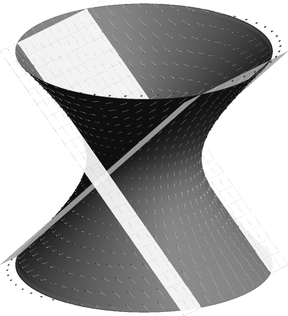
Figure 1. The surface $\mathcal{M}_{\mathrm{dS}}$ in the case $d=1$. Also shown is the Lorentz boost vector field $\Lambda_{(2)}$ and the hyperplanes $x^{0}=\pm x^{2}$. As one sees that hyperplanes divide $\mathcal{M}_{\mathrm{dS}}$ into six open regions, inside four of which $\Lambda_{(2)}$ is space-like, and in the other two $\Lambda_{(2)}$ is time-like. Along the hyperplanes $\Lambda_{(2)}$ has vanishing Minkowskian length, and the vector field vanishes exactly at the intersection of the two hyperplanes.

This hypersurface orthogonality translates into a static decomposition of the metric. Fix now our attention to the vector field $\Lambda_{(d+1)}$ and a corresponding set on which it is time-like. On this set ($\{x^{d+1}>\left\lvert x^{0}\right\rvert\}\cap\mathcal{M}_{\mathrm{dS}}$) define the coordinates $\zeta,\rho,z^{i}$ for $i\in\{1,\dots,d\}$ and $\sum_{i=1}^{d}(z^{i})^{2}=1$ (so $z^{i}$ describes the unit sphere in $\mathbb{R}^{d}$) by

(3.3) $$x^{\mu}=\begin{cases}\sqrt{1-\rho^{2}}\sinh(\zeta)&\mu=0\\ \sqrt{1-\rho^{2}}\cosh(\zeta)&\mu=d+1\\ \rho z^{\mu}&\mu\in\{1,\dots,d\}\end{cases}.$$

In this coordinate system the induced metric on $\mathcal{M}_{\mathrm{dS}}$ takes the form

(3.4) $$-(1-\rho^{2})\mathrm{d}{\zeta}^{2}+\frac{1}{1-\rho^{2}}\mathrm{d}{\rho}^{2}+\rho^{2}\mathrm{d}{\omega}^{2}_{\mathbb{S}^{d-1}}$$

which is spherically symmetric and explicitly independent of $\zeta$.

The boundary of the region $\{x^{d+1}>\left\lvert x^{0}\right\rvert\}$ corresponds to $\rho\to\pm 1$, at which point our coordinate system becomes degenerate. This is a manifestation of the cosmological horizon that is present in $\mathcal{M}_{\mathrm{dS}}$, and is related to the fact that this region is globally hyperbolic. This endows $\mathcal{M}_{\mathrm{dS}}$ with a rather different asymptotic causal structure when compared to Minkowski space $\mathbb{R}^{1,d}$.

On Minkowski space, let $\gamma_{1,2}:\mathbb{R}\to\mathbb{R}^{1,d}$ represent the worldline of two inertial observers; in other words $\gamma_{1,2}$ represent two time-like straight lines parametrised by arc-length. We have the following nice property: for every $s_{1}\in\mathbb{R}$, there exists $s_{2}\in\mathbb{R}$ such that $\gamma_{1}(s_{1})$ is in the causal past of $\gamma_{2}(s)$ for every $s>s_{2}$. This property is no longer true on $\mathcal{M}_{\mathrm{dS}}$. In particular, if we let $\omega$ be a unit vector in $\mathbb{R}^{d+1}$, we can consider the geodesic $\gamma_{\omega}:t\mapsto(t,\sqrt{1+t^{2}}\omega)$ curve along $\mathcal{M}_{\mathrm{dS}}$. For every distinct pair $\omega_{1},\omega_{2}$, there exists $\tilde{t}_{1},\tilde{t}_{2}$ such that for all $t_{1}>\tilde{t}_{1}$ and $t_{2}>\tilde{t}_{2}$, $\gamma_{\omega_{2}}(t_{2})$ is not in the causal past of $\gamma_{\omega_{1}}(t_{1})$ and vice versa.

The presence of this cosmological horizon has important consequences for the solutions of wave equations on a $\mathcal{M}_{\mathrm{dS}}$ background. Most notably is the fact that “structures” on a fixed “scale” tend to be frozen in place after finite time. One sees this already in Figure 1. Fix $\tilde{x}^{0}\geq 0$. Consider the wave equation on $\mathcal{M}_{\mathrm{dS}}$ to the future of $\tilde{x}^{0}$ with initial data prescribed on the sphere $\{x^{0}=\tilde{x}^{0}\}$. As already evident in Figure 1, by a domain of dependence argument the portion of the solution inside the set $\{x^{d+1}>\left\lvert x^{0}\right\rvert\}$ is entirely independent of the portion of the solution inside the set $\{x^{d+1}<-\left\lvert x^{0}\right\rvert\}$, as each of the two sets are future globally hyperbolic. Noting that $\tilde{x}^{0}$ gets larger and larger, the set $\{x^{d+1}>\left\lvert x^{0}\right\rvert\}$ takes up smaller and smaller angular size of the constant $\tilde{x}^{0}$ spheres, we see that we can divide $\mathcal{M}_{\mathrm{dS}}\cap\{x^{0}\geq\tilde{x}^{0}\}$ into more and more of these “mutually independent regions”. As we shall see in the remainder of this section, this feature of $\mathcal{M}_{\mathrm{dS}}$ background introduces an obstacle to parametrizing the asymptotic behaviour of $\mathrm{C}_{+}\mathrm{MC}$ manifolds using a finite dimensional modulation space.

We conclude this subsection with a small computation that will be useful later. Let $\tau$ be the unit future time-like vector field along $\mathcal{M}_{\mathrm{dS}}$ that is orthogonal to its constant $x^{0}$ slices; in terms of the coordinate system of $\mathbb{R}^{1,1+d}$ we easily verify that

(3.5) $$\tau=\left\langle x^{0}\right\rangle\partial_{x^{0}}+\sum_{i=1}^{d}\frac{x^{0}x^{i}}{\left\langle x^{0}\right\rangle}\partial_{x^{i}}=\sum_{i=1}^{d}\frac{x^{i}}{\left\langle x^{0}\right\rangle}\Lambda_{(i)}.$$

Indeed $\tau$ is in the span of the radial vector $\sum_{1}^{d}x^{i}\partial_{x^{i}}$ and the time-like vector $\partial_{x^{0}}$ so is orthogonal to the constant $x^{0}$ slices, which are round spheres. It is tangent to $\mathcal{M}_{\mathrm{dS}}$ as it is a linear combination of $\Lambda_{(i)}$ which are tangent vector fields. And a direct computation shows its Minkowskian length is $-1$. A further computation shows that $\tau$ is a geodesic vector field along $\mathcal{M}_{\mathrm{dS}}$.

As $\tau$ is unit and orthogonal to the constant $x^{0}$ hypersurfaces, its covariant derivative along said hypersurfaces is the shape tensor (see Appendix A.2), and so is related to the second fundamental form of the constant $x^{0}$ slices. Examining the definition of the second fundamental form, and considering the nested embedding of the constant $x^{0}$ slices into $\mathcal{M}_{\mathrm{dS}}$ and $\mathcal{M}_{\mathrm{dS}}$ into $\mathbb{R}^{1,d+1}$, we have that the second fundamental form of the constant $x^{0}$ slices inside $\mathcal{M}_{\mathrm{dS}}$ is just the projection of the second fundamental form of the corresponding round sphere (which has radius $\left\langle x^{0}\right\rangle$) in $\mathbb{R}^{1,d+1}$ onto $\mathcal{M}_{\mathrm{dS}}$. Thus we have derived

Proposition 3.1.

Let $\mathring{\nabla}$ denote the induced Levi-Civita connection along $\mathcal{M}_{\mathrm{dS}}$, and let $\tau$ as above. Then

$$\mathring{\nabla}_{b}\tau^{c}=\frac{x^{0}}{\left\langle x^{0}\right\rangle}(\delta^{c}_{b}+\tau_{b}\tau^{c})$$

where $\tau_{b}=\mathring{g}_{ba}\tau^{a}$ is the metric dual of $\tau$ via the induced metric $\mathring{g}$ on $\mathcal{M}_{\mathrm{dS}}$.

3.2. Linear “instability” of $\mathcal{M}_{\mathrm{dS}}$ without modulation

Going back to the $\mathrm{C}_{+}\mathrm{MC}$ problem, let us consider a small perturbation of $\mathcal{M}_{\mathrm{dS}}$ as a graph over it. More precisely, we consider the manifold $M_{\phi}=\left\{\;\vec{x}+\phi(\vec{x})\vec{n}\;\middle|\;\vec{x}\in\mathcal{M}_{\mathrm{dS}}\;\right\}$ where $\phi:\mathcal{M}_{\mathrm{dS}}\to\mathbb{R}$ is some smooth function. In Appendix A.5 we compute the mean curvature of $M_{\phi}$ and its formal linearisation. The linearised equation for $\phi$ such that $M_{\phi}$ has constant mean curvature $d+1$ is given by (A.13), which we reproduce here

$$\Box_{\mathcal{M}_{\mathrm{dS}}}\phi+(d+1)\phi=0.$$

In this subsection we study the asymptotic behaviour of solutions to this linearised equation.

Equation (A.13) takes the form of a Klein-Gordon equation but with negative mass. Experience with static space-times (such as Minkowski space) tells us that wave equations with sufficiently negative potentials will exhibit generically exponential growth of the solution. This is clear when we write the equations in the form

$$\partial_{\zeta}^{2}\phi=-L\phi$$

where $L$ is a time-independent Schrödinger operator whose spectrum protrudes into the negative real axis. As we have seen in the previous subsection, the induced metric on $\mathcal{M}_{\mathrm{dS}}$ in fact admits such a static decomposition, if we restrict to a region where a given Lorentz boost vector field is time-like. Furthermore, the spherical symmetry of the static decomposition (3.4) implies that the exponential growth of the solution to the equation also induces exponential growth of (some of) the derivatives.

One may however argue that the $(\zeta,\rho,z^{i})$ coordinate system of (3.4), in addition to not covering the entirety of $\mathcal{M}_{\mathrm{dS}}$ without degeneration, is also not representative of the true asymptotic behaviour of a $\mathrm{C}_{+}\mathrm{MC}$ manifold, due to the fact that every constant $\zeta$ slice passes through the sphere $x^{0}=x^{d+1}=0$, and so the behaviour of the solution as $\zeta\to\infty$ may not be reflective of what we physically think of as asymptotic behaviour, where $x^{0}\to\infty$. With regards to the “true” asymptotic behaviour, one may expect something better. This is in view of known results concerning the wave and (positive-mass) Klein-Gordon equations on de Sitter backgrounds (see e.g. [MSBV14] and references therein) that suggest one expects the solution itself to converge to a (possibly non-zero) constant, with decaying derivatives. One may hope that even in the case of the negative-mass Klein-Gordon term, the derivatives obey certain improved decay or boundedness properties compared to the unboundedly growing solution.

To understand the more physically relevant asymptotics, we first write down explicitly the operator $\Box_{\mathcal{M}_{\mathrm{dS}}}$ in coordinates. Let $t=x^{0}$ and $\omega$ be some coordinate system for the sphere $\mathbb{S}^{d}$, the metric for $\mathcal{M}_{\mathrm{dS}}$ in this cylindrical coordinate system can be expressed as

(3.5) $$-\frac{1}{\left\langle t\right\rangle^{2}}\mathrm{d}{t}^{2}+\left\langle t\right\rangle^{2}\mathrm{d}{\omega}^{2},$$

from which we can write down the wave operator as

(3.6) $$\Box_{\mathcal{M}_{\mathrm{dS}}}\phi=-\frac{1}{\left\langle t\right\rangle^{d-1}}\partial_{t}\left(\left\langle t\right\rangle^{d+1}\partial_{t}\phi\right)+\frac{1}{\left\langle t\right\rangle^{2}}\not{\triangle}\phi$$

where $\not{\triangle}$ is the spherical Laplacian on $\mathbb{S}^{d}$. The spherical symmetry allows us to decompose a solution based on angular momentum $\ell$, which is a non-negative integer. For a solution with angular momentum $\ell$, which we denote by $\psi_{\ell}$, we have that

$$\not{\triangle}\psi_{\ell}=-\ell(\ell+d+1)\psi_{\ell}.$$

3.2.1. Spherically symmetric case

For $\ell=0$, the linearised $\mathrm{C}_{+}\mathrm{MC}$ equation (A.13) reduces via (3.6) to the ODE

$$\left\langle t\right\rangle^{2}\psi_{0}^{\prime\prime}+(d+1)t\psi_{0}^{\prime}=(d+1)\psi_{0}.$$

Substituting $\psi_{0}=t\hat{\psi}_{0}$ we get

$$\left\langle t\right\rangle^{2}(t\hat{\psi}_{0}^{\prime\prime}+2\hat{\psi}_{0}^{\prime})+(d+1)t(t\hat{\psi}_{0}^{\prime}+\hat{\psi}_{0})=(d+1)t\hat{\psi}_{0}$$

which gives us the following equation for $f=\hat{\psi}_{0}^{\prime}$:

(3.7) $$\left\langle t\right\rangle^{2}tf^{\prime}+2\left\langle t\right\rangle^{2}f+(d+1)t^{2}f=0.$$

This equation we can explicitly integrate

$$\frac{f^{\prime}}{f}=-\frac{2}{t}-\frac{(d+1)t}{\left\langle t\right\rangle^{2}}\implies\log f+C=-2\log t-(d+1)\log\left\langle t\right\rangle$$

or

(3.8) $$\hat{\psi}_{0}^{\prime}=\frac{C}{t^{2}\left\langle t\right\rangle^{d+1}}.$$

The case $C=0$ corresponds to $\hat{\psi}_{0}=C^{\prime}$ and hence $\psi_{0}=C^{\prime}t$. This solution corresponds to the temporal translation symmetry of the background $\mathbb{R}^{1,d+1}$. Note that in terms of the “proper time” for the constant $\omega$ observers in $\mathcal{M}_{\mathrm{dS}}$, the linear in $t$ growth translates to an exponential growth.

The equation (3.8) shows that $\hat{\psi}_{0}^{\prime}$ is integrable as $t\to\infty$ and so we have that $\hat{\psi}_{0}$ converges to a finite constant generically, and signals the generic linear in $t$ growth of a solution, agreeing with our analysis in Section 2. We summarise the results as

Proposition 3.2.

For spherically symmetric perturbations, the solutions $\psi_{0}$ to the linearised equation grows linearly in $t$ generically. The renormalised quantity $\frac{1}{t}\psi_{0}$ is bounded, and its first derivative decays; this is while the derivative $\psi^{\prime}_{0}$ generically remains bounded but does not decay.

3.2.2. Higher angular momentum case

For $\ell>0$, instead of commuting with the $t$ weight, we commute with a $\left\langle t\right\rangle$ weight. Writing $\varphi=\left\langle t\right\rangle\breve{\varphi}$ we have

$$\Box_{\mathcal{M}_{\mathrm{dS}}}\varphi+(d+1)\varphi=\left\langle t\right\rangle\left[\Box_{\mathcal{M}_{\mathrm{dS}}}\breve{\varphi}-2t\partial_{t}\breve{\varphi}+\frac{d}{\left\langle t\right\rangle^{2}}\breve{\varphi}\right].$$

Multiplying the equation with $\left\langle t\right\rangle^{2-d}\partial_{t}\breve{\varphi}$ and integrating against the space-time volume form $\left\langle t\right\rangle^{d-1}\leavevmode\nobreak\ \mathrm{d}{t}\leavevmode\nobreak\ \mathrm{d}{\omega}$ we have

$$0 =\iint\left\langle t\right\rangle^{2}\left[\Box_{\mathcal{M}_{\mathrm{dS}}}\breve{\varphi}-2t\breve{\varphi}_{t}+\frac{d}{\left\langle t\right\rangle^{2}}\breve{\varphi}\right]\breve{\varphi}_{t}\leavevmode\nobreak\ \mathrm{d}{t}\leavevmode\nobreak\ \mathrm{d}{\omega}$$

$$=\iint-\frac{1}{2\left\langle t\right\rangle^{2d-2}}\partial_{t}\left(\left\langle t\right\rangle^{d+1}\breve{\varphi}_{t}\right)^{2}-\frac{1}{2}\partial_{t}\left(\breve{\varphi}_{\omega}^{2}-d\breve{\varphi}^{2}\right)-2t\left\langle t\right\rangle^{2}\breve{\varphi}_{t}^{2}\leavevmode\nobreak\ \mathrm{d}{t}\leavevmode\nobreak\ \mathrm{d}{\omega}$$

$$=\iint-\frac{1}{2}\partial_{t}\left(\left\langle t\right\rangle^{4}\breve{\varphi}_{t}^{2}+\breve{\varphi}_{\omega}^{2}-d\breve{\varphi}^{2}\right)-(d+1)t\left\langle t\right\rangle^{2}\breve{\varphi}_{t}^{2}\leavevmode\nobreak\ \mathrm{d}{t}\leavevmode\nobreak\ \mathrm{d}{\omega}$$

which implies

(3.9) $$\int\left\langle t\right\rangle^{4}\breve{\varphi}_{t}^{2}+\breve{\varphi}_{\omega}^{2}-d\breve{\varphi}^{2}\leavevmode\nobreak\ \mathrm{d}{\omega}\Big{]}^{t=T}_{0}=-2(d+1)\iint t\left\langle t\right\rangle^{2}\breve{\varphi}_{t}^{2}\leavevmode\nobreak\ \mathrm{d}{t}\leavevmode\nobreak\ \mathrm{d}{\omega}<0$$

provided we restrict to the forward region $t>0$. For the $\ell\geq 1$ spherical harmonics the energy quantity controlled is positive semi-definite; for $\ell>1$ the energy quantity is in fact coercive. The monotonicity of (3.9) already implies that, as long as we project out the spherically symmetric mode first, that $\int\left\langle t\right\rangle^{4}\breve{\varphi}_{t}^{2}\leavevmode\nobreak\ \mathrm{d}{\omega}$ remains bounded. This can be strengthened slightly: since $\int\left\langle t\right\rangle^{4}\breve{\varphi}_{t}^{2}\leavevmode\nobreak\ \mathrm{d}{\omega}$ is monotonically decreasing in $t$, the limit as $t\to\infty$ must exist. Suppose $\lim_{t\to\infty}\int\left\langle t\right\rangle^{4}\breve{\varphi}_{t}^{2}\leavevmode\nobreak\ \mathrm{d}{\omega}>0$, this gives asymptotically a lower bound

$$\int\left\langle t\right\rangle^{2}\breve{\varphi}_{t}^{2}\leavevmode\nobreak\ \mathrm{d}{\omega}\gtrsim\frac{1}{\left\langle t\right\rangle^{2}}$$

which would imply that the right hand side of (3.9) is not integrable in time, giving a contradiction. Therefore we have that

Proposition 3.3.

When $\ell\geq 1$, we have that

$$\lim_{t\to\infty}\left\langle t\right\rangle^{2}\partial_{t}[\left\langle t\right\rangle^{-1}\psi_{\ell}(t)]=0,$$

which implies that the $\left\langle t\right\rangle^{-1}\psi_{\ell}(t)$ converges to a finite value for each fixed $\omega\in\mathbb{S}^{d}$, and that $\psi_{\ell}$ grows at most linearly.

Remark 3.4.

For the special case $\ell=1$, for each fixed $\omega$, the renormalised quantity $\left\langle t\right\rangle^{-1}\psi_{1}(t,\omega)$ is such that its time derivative is spanned by $\{0,\left\langle t\right\rangle^{-d-3}\}$. The former corresponds to $\psi_{1}(t,\omega)=\psi_{1}(0,\omega)\left\langle t\right\rangle$, which is the linear instability associated with the spatial translation symmetries of $\mathbb{R}^{1,d+1}$. Of the symmetries in the Poincaré group, only the translations do not fix $\mathcal{M}_{\mathrm{dS}}$; the indefinite orthogonal group $O(1,d+1)$ generates no additional linear instabilities.

This, however, should not be interpreted as the non-existence of additional linear instabilities. In fact, as we will see immediately below, (3.9) and the linear upper bound for $\psi_{\ell}$ in Proposition 3.3 are as good as we can get.

3.3. Cosmological horizon and a no-go result

Playing with a domain of dependence argument using the presence of cosmological horizons on $\mathcal{M}_{\mathrm{dS}}$ and the instability in the spherically symmetric cases gives us immediately

1. linear mode instability for infinitely many angular momenta (Theorem 3.5), and

2. a no-go theorem for approximating the asymptotic profile of perturbed solutions using directly $\mathcal{M}_{\mathrm{dS}}$ and its images under the Poincaré group (Theorem 3.6).

The first result indicates that were one to try to naïvely approach the $\mathrm{C}_{+}\mathrm{MC}$ stability problem from the point of view of modulation theory applied to the set-up where the solution manifold $M_{\phi}$ is regarded as a graph in the normal bundle of $\mathcal{M}_{\mathrm{dS}}$, one will necessarily have to contend with an infinite dimensional family of modulations. The second result shows that in the non-spherically-symmetric case, the asymptotic behaviour of solutions should be more complicated than suggested by Corollary 2.17 and Theorem 2.22.

Theorem 3.5.

Let $Y_{m,\ell}$ denote spherical harmonics for $\mathbb{S}^{d}$. Let $\{(m_{\alpha},\ell_{\alpha})\}$ be a fixed, finite set of parameters. Then there exists a solution to (A.13) satisfying

$$\left\lVert\phi(t)\right\rVert_{L^{\infty}(\mathbb{S}^{d})}\gtrsim t$$

for all sufficiently large $t$, and that

$$\int_{\mathbb{S}^{d}}\phi(t,\omega)Y_{m_{\alpha},\ell_{\alpha}}(\omega)\leavevmode\nobreak\ \mathrm{d}{\omega}=0$$

for parameters belonging to our fixed finite set.

Proof.

Let $N>\#\{(m_{\alpha},\ell_{\alpha})\}$ and choose $N$ distinct points on $\mathbb{S}^{d}$ labelled $\{\omega_{1},\dots,\omega_{N}\}$. Let $\delta_{0}=\min_{i\neq j}\left\lvert\omega_{i}-\omega_{j}\right\rvert$. Fix $t_{0}\geq 8/\delta_{0}$. Consider the sets

$$B_{i}(r)=\left\{\;(t_{0},\omega)\in\mathcal{M}_{\mathrm{dS}}\;\middle|\;\left\lvert\omega-\omega_{i}\right\rvert<r\;\right\},$$

by our discussion of the cosmological horizon above, we see that there exists $\rho_{0}>0$ such that,

• $B_{i}(2\rho_{0})$ are mutually disjoint;

• the domain of dependence for $B_{i}(\rho_{0})$ contains the ray $\left\{\;(t,\omega_{i})\;\middle|\;t\geq t_{0}\;\right\}$.

Now let $\phi_{i}^{(0)}:\{t_{0}\}\times\mathbb{S}^{d}\to\mathbb{R}$ be a smooth bump function supported on $B_{i}(2\rho_{0})$ and such that $\phi_{i}^{(0)}=1$ on $B_{i}(\rho_{0})$. Consider the Cauchy problem for (A.13) with initial data prescribed on $\{t_{0}\}\times\mathbb{S}^{d}$ such that

$$\phi|_{t_{0}}=\sum_{i=1}^{N}\epsilon_{i}t_{0}\phi_{i}^{(0)},\qquad\text{and}\qquad\partial_{t}\phi|_{t_{0}}=\sum_{i=1}^{N}\epsilon_{i}\phi_{i}^{(0)}.$$

We have the inside the domain of dependence of $B_{i}(\rho_{0})$, and in particular along the ray $[t_{0},\infty)\times\{\omega_{i}\}$, solution coincides with the spherically symmetric solution $\phi(t,\omega)=\epsilon_{i}t$, and hence as long as for some $\epsilon_{i}$ we have that $\epsilon_{i}\neq 0$, we have the lower bound on the $L^{\infty}$ norm as claimed.

It remains to verify the assumption on the spherical harmonics. But the condition on the spherical harmonics reduce to a family of $\#\{(m_{\alpha},\ell_{\alpha})\}$ linear equations which can be solved for generic choices of $\omega_{i}$, and with the prescription $\epsilon_{1}=1$. ∎

Theorem 3.6.

Suppose the full $\mathrm{C}_{+}\mathrm{MC}$ problem, as a perturbation of $\mathcal{M}_{\mathrm{dS}}$, has small data global existence. Then there exist $\mathrm{C}_{+}\mathrm{MC}$ manifolds which are not eventually tangent to a light cone. More precisely, fix a initial time $t_{0}>0$, then there exist a $\mathrm{C}_{+}\mathrm{MC}$ manifold $M$, which can be chosen to be arbitrarily close to $\mathcal{M}_{\mathrm{dS}}$ at time $t_{0}$, such that for every $(\tau_{0},\xi_{0})\in\mathbb{R}^{1,1+d}$ we have

$$\lim_{t\to\infty}\sup_{(t,x)\in M}\left\lvert\left\lvert x-\xi_{0}\right\rvert-t+\tau_{0}\right\rvert>0.$$

Proof.

Consider the initial data as a graph over the $t_{0}$ slice of $\mathcal{M}_{\mathrm{dS}}$. Since $t_{0}>0$, we can choose initial data at $t_{0}$ such that restricted to the set $\{x^{d+1}\geq\sqrt{1+t_{0}^{2}}\}$ agree with the spatial translation of $\mathcal{M}_{\mathrm{dS}}$ in the positive $x^{d+1}$ direction by distance $\epsilon$, and such that restricted to the set $\{x^{d+1}\leq-\sqrt{1+t_{0}^{2}}\}$ agree with the spatial translation of $\mathcal{M}_{\mathrm{dS}}$ in the negative $x^{d+1}$ direction by distance $\epsilon$, and smoothly joined in between. Our assumption of small data global existence implies that for sufficiently small $\epsilon$ the Cauchy problem given this initial data can be solved globally. In the relevant domains of dependence, which in particular will contain a small neighbourhood of the curves with $x^{1}=\cdots=x^{d}=0$ and $t>t_{0}$ the solution will agree with the two spatially translated solutions. From this we see that for any $t>t_{0}$ the quantity

$$\sup_{(t,x)\in M}\left\lvert\left\lvert x-\xi_{0}\right\rvert-t+\tau_{0}\right\rvert>\epsilon/2.\qed$$

Remark 3.7.

That $t_{0}>0$ is only for convenience. The data can be chosen to be arbitrarily close to that of $\mathcal{M}_{\mathrm{dS}}$ at any one fixed time by a Cauchy stability argument. By choosing larger $t_{0}$ we can also include more “pieces” of translated solutions, as is done in the proof to Theorem 3.5. This shows that the asymptotic profiles for the full problem is also, in some sense, infinite dimensional, in accordance to the idea that the cosmological horizon freezes in perturbations after finite time.

Remark 3.8.

For the last inequality in the proof of Theorem 3.6 to hold we used that $\mathcal{M}_{\mathrm{dS}}$ is ruled by null geodesics. Thus as $t\to\infty$, while the angular size of the set $\{x^{d+1}\geq\sqrt{1+t_{0}^{2}}\}\cap\mathcal{M}_{\mathrm{dS}}$ gets smaller and smaller, the physical “diameter” of this set at a fixed time remains roughly constant.

Observe in the statement of Theorem 3.6 that small data global existence is assumed. One may ask whether it is possible to prove this fact independently of asymptotic stability (which is false in the graphical setting in view of Theorem 3.6). In the graphical setting Theorem 3.5 suggests that this would be difficult. In fact, in view of Theorem 3.5, the asymptotics given by Proposition 3.3 implies that $\partial_{t}\phi(t)$ for a generic solution of (A.13) converges to a non-zero constant (for each fixed $\omega$). This poses a severe obstacle to studying the $\mathrm{C}_{+}\mathrm{MC}$ problem in the formulation of a quasilinear wave equation for a graph over the normal bundle of $\mathcal{M}_{\mathrm{dS}}$. Nevertheless, as we shall see in the remainder of this paper, the desired small data global existence is in fact true, and we can also obtain some control over the asymptotic behaviour of the solutions.

4. Inverse-Gauss-map gauge

The linear analysis of Section 3.2 leaves still a ray of hope: while the analysis shows that treating a $\mathrm{C}_{+}\mathrm{MC}$ manifold which is a perturbation of $\mathcal{M}_{\mathrm{dS}}$ as a graph over its normal bundle leads to great difficulties in studying the associated quasilinear wave equations, it also shows that certain renormalised quantities behave better. In particular, (3.9) gives derivative control over the rescaled solution $\left\langle t\right\rangle^{-1}\phi$ to (A.13). One approach to the $\mathrm{C}_{+}\mathrm{MC}$ stability problem would be to derive the equation for this rescaled quantity, and hope that its equation of motion can be studied perturbatively under this derivative decay. Here we take an alternative approach. Instead of treating a $\mathrm{C}_{+}\mathrm{MC}$ manifold as a graph over the normal bundle of $\mathcal{M}_{\mathrm{dS}}$, we introduce in this section the inverse-Gauss-map gauge. In this gauge the evolution equation for the $\mathrm{C}_{+}\mathrm{MC}$ problem is most naturally expressed in terms of the Codazzi equations for the embedding, which is automatically at the derivative level compared to the graphical formulation. In other words, by reformulating the question in a geometric manner, we will be able to avoid some of the difficulties that manifest in the graphical treatment of the problem.

For a time-like hypersurface $M$ of $\mathbb{R}^{1,d+1}$, the Gauss map is a (smooth) map $G:M\to\mathcal{M}_{\mathrm{dS}}$, where the value of $G$ corresponds to the out-ward unit-normal of the hypersurface (see Appendix A.3). We will consider the regime in which $G$ is a diffeomorphism onto its image; this will be the case, for example, if we have a sufficiently small perturbation of $\mathcal{M}_{\mathrm{dS}}$ (see Remark 4.6 below). We let $\Phi$ denote the inverse map to $G$ in this case.

Now, using the ambient geometry of $\mathbb{R}^{1,d+1}$ we can naturally identify the tangent spaces $T_{p}M$ and $T_{G(p)}\mathcal{M}_{\mathrm{dS}}$. Note that this identification is different from the identification afforded by the derivative map $\mathrm{d}{G}$ or $\mathrm{d}\Phi$. Under this identification we observe that $\mathrm{d}{G}$ as well as $\mathrm{d}\Phi$ can each be interpreted as a $(1,1)$-tensor on $TM$ and $T\mathcal{M}_{\mathrm{dS}}$ respectively. By the inverse-Gauss-map gauge we mean that $M$ is studied as the image of $\mathcal{M}_{\mathrm{dS}}$ under the mapping $\Phi$, and its geometry studied through the “tensor field” $\mathrm{d}\Phi$.

In classical differential geometry (see also Appendices A.2 and A.3) it is well-known that the differential of the Gauss map is the shape operator. Using the identification above, as well as the fact that $\mathrm{d}{G}\circ\mathrm{d}{\Phi}=\mathbf{1}$, we see that the first and second fundamental forms, which we now write as $g$ and $k$, of $M$ as a hypersurface in $\mathbb{R}^{1,d+1}$ can be expressed as tensor fields over $\mathcal{M}_{\mathrm{dS}}$, where $\mathring{g}$ is the metric of $\mathcal{M}_{\mathrm{dS}}$. For convenience we also write $A_{a}^{b}=(\mathrm{d}\Phi)_{a}^{b}$ the $(1,1)$-tensor interpretation of the deformation.

(4.1) $$g_{ab} =\mathring{g}_{cd}A_{a}^{c}A_{b}^{d}$$

(4.2) $$k_{ab} =\mathring{g}_{ac}A_{b}^{c}.$$

The second fundamental form $k_{ab}$ is symmetric. The equation of motion that we will be studying then arises from the Codazzi equations of the embedding $M\to\mathbb{R}^{1,d+1}$, which reads

(4.3) $$\nabla_{a}k_{bc}-\nabla_{b}k_{ac} =0,$$

(4.4) $$g^{ac}\nabla_{a}k_{bc} =0.$$

The equation (4.3) is a direction consequence of Codazzi equation using that $\mathbb{R}^{1,d+1}$ is flat, and contains within it the integrability condition that “$\mathrm{d}{\mathrm{d}\Phi}=0$”; on the other hand (4.4) is obtained from taking the $g$ trace of (4.3) and using the condition that $\operatorname{tr}_{g}k=d+1$ is constant for our solution.

The system (4.3) and (4.4) clearly forms a quasilinear divergence-curl system for the unknown $A_{a}^{b}$, and in this form already exhibits the hyperbolic nature of the equations; it also has some formal similarity with the systems of nonlinear electrodynamics. As we are interested in the case of perturbations of $\mathcal{M}_{\mathrm{dS}}$, we observe that our $A_{a}^{c}$ can be written as the perturbation $A_{a}^{c}=\delta_{a}^{c}+\phi_{a}^{c}$, with $\phi\equiv 0$ being the specific $\mathcal{M}_{\mathrm{dS}}$ solution.

For convenience we will also write $\phi_{ab}=\mathring{g}_{ac}\phi^{c}_{b}$, we have that by assumption $k_{ab}=\mathring{g}_{ab}+\phi_{ab}$, and hence $\phi_{ab}$ is a symmetric two-tensor.

We will write $\Gamma_{ab}^{c}$ for the Christoffel symbols of $g_{ab}$ relative to the background metric $\mathring{g}_{ab}$, that is to say

(4.5) $$\Gamma_{ab}^{c}\overset{\mbox{\tiny{def}}}{=}\frac{1}{2}g^{cd}\left(\mathring{\nabla}_{a}g_{bd}+\mathring{\nabla}_{b}g_{ad}-\mathring{\nabla}_{d}g_{ab}\right)$$

where $\mathring{\nabla}$ is the Levi-Civita connection relative to the metric $\mathring{g}$. Observe that $\Gamma$ is at the level of one derivative of $\phi$: this could potentially cause a bit of problem with expansion of the equations. Fortunately we have some nice cancellations that comes in to play. In the remaining part of this section we will re-write the equations of motion (4.3) and (4.4) in terms of $\phi$ and the fixed background $\mathring{g}$.

First we expand $\Gamma_{ab}^{c}$, using that $\mathring{\nabla}\mathring{g}=0$, and that

(4.6) $$g_{ab}=\mathring{g}_{ab}+2\phi_{ab}+\phi_{ad}\phi^{d}_{b}.$$

We have

$$\Gamma_{ab}^{c}=\frac{1}{2}g^{cd}\big{[}\mathring{\nabla}_{a}(2\phi_{bd}+\phi_{bf}\phi_{d}^{f})+\mathring{\nabla}_{b}(2\phi_{ad}+\phi_{af}\phi_{d}^{f})-\mathring{\nabla}_{d}(2\phi_{ab}+\phi_{bf}\phi_{a}^{f})\big{]}.$$

So (4.3) becomes

$$0 =\nabla_{a}k_{bc}-\nabla_{b}k_{ac}$$

$$=\mathring{\nabla}_{a}\phi_{bc}-\mathring{\nabla}_{b}\phi_{ac}-\Gamma_{ab}^{e}k_{ec}-\Gamma_{ac}^{e}k_{be}+\Gamma_{ba}^{e}k_{ec}+\Gamma_{bc}^{e}k_{ae}$$

$$=\mathring{\nabla}_{a}\phi_{bc}-\mathring{\nabla}_{b}\phi_{ac}-\Gamma_{ac}^{e}k_{be}+\Gamma_{bc}^{e}k_{ae}$$

$$=\mathring{\nabla}_{a}\phi_{bc}-\mathring{\nabla}_{b}\phi_{ac}$$

$$\qquad-\frac{1}{2}g^{ef}\left[\mathring{\nabla}_{a}(2\phi_{cf}+\phi_{ch}\phi_{f}^{h})+\mathring{\nabla}_{c}(2\phi_{af}+\phi_{ah}\phi_{f}^{h})-\mathring{\nabla}_{f}(2\phi_{ac}+\phi_{ch}\phi_{a}^{h})\right]k_{be}$$

$$\qquad+\frac{1}{2}g^{ef}\left[\mathring{\nabla}_{b}(2\phi_{cf}+\phi_{ch}\phi_{f}^{h})+\mathring{\nabla}_{c}(2\phi_{bf}+\phi_{bh}\phi_{f}^{h})-\mathring{\nabla}_{f}(2\phi_{bc}+\phi_{ch}\phi_{b}^{h})\right]k_{ae}$$

Now we use the following: let $\psi_{a}^{c}$ be such that

(4.7) $$(\delta_{a}^{c}+\psi_{a}^{c})(\delta_{c}^{b}+\phi_{c}^{b})=\delta_{a}^{b}$$

For $\phi$ sufficiently small this exists as the linear mapping $A$ is invertible. This in particular implies that $\psi\phi=\phi\psi$ (they commute). We have that by definition

(4.8) $$g^{ef}=(\delta_{a}^{f}+\psi_{a}^{f})\mathring{g}^{ab}(\delta_{b}^{e}+\psi_{b}^{e}),$$

so that

(4.9) $$g^{ef}k_{ae}=\delta_{a}^{f}+\psi_{a}^{f}.$$

Note that (4.9) implies, via our assumption that $\operatorname{tr}_{g}k=d+1$, that

(4.10) $$\operatorname{tr}\psi=\psi_{a}^{a}=0,$$

this in turn implies that

(4.11) $$\phi_{a}^{a}+\phi_{a}^{b}\psi_{b}^{a}=0.$$

Remark 4.1.

The equations (4.10) and (4.11) forces certain constraints on the prescribed initial data. More precisely, we should think that the free data to be prescribed would be $\psi$, which satisfies (4.10) and from which we can think about $\phi$. One can equivalently write down the equation for $\psi$; however it seems that the equations for $\phi$ is somewhat simpler than that of $\psi$.

Remark 4.2.

Observe that in (4.11), since $\psi$ is trace-free, we can decompose $\phi=\hat{\phi}+\tilde{\phi}$, and similarly $\psi=\hat{\psi}+\tilde{\psi}$, into pure-trace and traceless parts. (4.10) says that $\hat{\psi}=0$. The identity (4.11) becomes $\operatorname{tr}\hat{\phi}+\tilde{\phi}:\tilde{\psi}=0$, indicating that the trace part of $\phi$ should be “quadratic” in size compared to the trace-free part.

Using this decomposition we expand (4.3) to get

$$0 =\mathring{\nabla}_{a}\phi_{bc}-\mathring{\nabla}_{b}\phi_{ac}$$

$$\qquad-\frac{1}{2}\left[\mathring{\nabla}_{a}(2\phi_{cf}+\phi_{ch}\phi_{f}^{h})+\mathring{\nabla}_{c}(2\phi_{af}+\phi_{ah}\phi_{f}^{h})-\mathring{\nabla}_{f}(2\phi_{ac}+\phi_{ch}\phi_{a}^{h})\right](\delta_{b}^{f}+\psi_{b}^{f})$$

$$\qquad+\frac{1}{2}\left[\mathring{\nabla}_{b}(2\phi_{cf}+\phi_{ch}\phi_{f}^{h})+\mathring{\nabla}_{c}(2\phi_{bf}+\phi_{bh}\phi_{f}^{h})-\mathring{\nabla}_{f}(2\phi_{bc}+\phi_{ch}\phi_{b}^{h})\right](\delta_{a}^{f}+\psi_{a}^{f})$$

$$=-\mathring{\nabla}_{a}\phi_{bc}+\mathring{\nabla}_{b}\phi_{ac}-\mathring{\nabla}_{a}(\phi_{ch}\phi_{b}^{h})+\mathring{\nabla}_{b}(\phi_{ch}\phi_{a}^{h})$$

$$\qquad-\frac{1}{2}\left[\mathring{\nabla}_{a}(2\phi_{cf}+\phi_{ch}\phi_{f}^{h})+\mathring{\nabla}_{c}(2\phi_{af}+\phi_{ah}\phi_{f}^{h})-\mathring{\nabla}_{f}(2\phi_{ac}+\phi_{ch}\phi_{a}^{h})\right]\psi_{b}^{f}$$

$$\qquad+\frac{1}{2}\left[\mathring{\nabla}_{b}(2\phi_{cf}+\phi_{ch}\phi_{f}^{h})+\mathring{\nabla}_{c}(2\phi_{bf}+\phi_{bh}\phi_{f}^{h})-\mathring{\nabla}_{f}(2\phi_{bc}+\phi_{ch}\phi_{b}^{h})\right]\psi_{a}^{f}$$

$$=-\mathring{\nabla}_{a}\phi_{bc}+\mathring{\nabla}_{b}\phi_{ac}-\mathring{\nabla}_{a}(\phi_{ch}\phi_{b}^{h})+\mathring{\nabla}_{b}(\phi_{ch}\phi_{a}^{h})$$

$$\qquad-\left[\mathring{\nabla}_{a}\phi_{cf}+\mathring{\nabla}_{c}\phi_{af}-\mathring{\nabla}_{f}\phi_{ac}\right]\psi_{b}^{f}+\left[\mathring{\nabla}_{b}\phi_{cf}+\mathring{\nabla}_{c}\phi_{bf}-\mathring{\nabla}_{f}\phi_{bc}\right]\psi_{a}^{f}$$

$$\qquad-\frac{1}{2}\left[\mathring{\nabla}_{a}(\phi_{ch}\phi_{f}^{h})+\mathring{\nabla}_{c}(\phi_{ah}\phi_{f}^{h})-\mathring{\nabla}_{f}(\phi_{ch}\phi_{a}^{h})\right]\psi_{b}^{f}$$

$$\qquad+\frac{1}{2}\left[\mathring{\nabla}_{b}(\phi_{ch}\phi_{f}^{h})+\mathring{\nabla}_{c}(\phi_{bh}\phi_{f}^{h})-\mathring{\nabla}_{f}(\phi_{ch}\phi_{b}^{h})\right]\psi_{a}^{f}$$

$$=-\mathring{\nabla}_{a}\phi_{bc}+\mathring{\nabla}_{b}\phi_{ac}-\mathring{\nabla}_{a}(\phi_{ch}\phi_{b}^{h})+\mathring{\nabla}_{b}(\phi_{ch}\phi_{a}^{h})$$

$$\qquad-\left[\mathring{\nabla}_{a}\phi_{cf}+\mathring{\nabla}_{c}\phi_{af}-\mathring{\nabla}_{f}\phi_{ac}\right]\psi_{b}^{f}+\left[\mathring{\nabla}_{b}\phi_{cf}+\mathring{\nabla}_{c}\phi_{bf}-\mathring{\nabla}_{f}\phi_{bc}\right]\psi_{a}^{f}$$

$$\qquad+\frac{1}{2}\left[\mathring{\nabla}_{a}\phi_{ch}+\mathring{\nabla}_{c}\phi_{ah}\right](\phi_{b}^{h}+\psi_{b}^{h})-\frac{1}{2}\left[\mathring{\nabla}_{b}\phi_{ch}+\mathring{\nabla}_{c}\phi_{bh}\right](\phi_{a}^{h}+\psi_{a}^{h})$$

$$\qquad-\frac{1}{2}\left[\phi_{ch}\mathring{\nabla}_{a}\phi_{f}^{h}+\phi_{ah}\mathring{\nabla}_{c}\phi_{f}^{h}-\mathring{\nabla}_{f}(\phi_{ch}\phi_{a}^{h})\right]\psi_{b}^{f}$$

$$\qquad+\frac{1}{2}\left[\phi_{ch}\mathring{\nabla}_{b}\phi_{f}^{h}+\phi_{bh}\mathring{\nabla}_{c}\phi_{f}^{h}-\mathring{\nabla}_{f}(\phi_{ch}\phi_{b}^{h})\right]\psi_{a}^{f}$$

where we used that $\phi\psi=\psi\phi=-\psi-\phi$. This allows us to further simplify

$$0 =-\mathring{\nabla}_{a}\phi_{bc}+\mathring{\nabla}_{b}\phi_{ac}$$

$$\qquad+\frac{1}{2}\left(\mathring{\nabla}_{c}\phi_{ah}-\mathring{\nabla}_{a}\phi_{ch}\right)\phi_{b}^{h}+\frac{1}{2}\left(\mathring{\nabla}_{b}\phi_{ch}-\mathring{\nabla}_{c}\phi_{bh}\right)\phi_{a}^{h}+\left(\mathring{\nabla}_{b}\phi_{ah}-\mathring{\nabla}_{a}\phi_{bh}\right)\phi_{c}^{h}$$

$$\qquad-\frac{1}{2}\left[\mathring{\nabla}_{a}\phi_{cf}+\mathring{\nabla}_{c}\phi_{af}-2\mathring{\nabla}_{f}\phi_{ac}\right]\psi_{b}^{f}+\frac{1}{2}\left[\mathring{\nabla}_{b}\phi_{cf}+\mathring{\nabla}_{c}\phi_{bf}-2\mathring{\nabla}_{f}\phi_{bc}\right]\psi_{a}^{f}$$

$$\qquad-\frac{1}{2}\left[\phi_{ch}(\mathring{\nabla}_{a}\phi_{f}^{h}-\mathring{\nabla}_{f}\phi_{a}^{h})+\phi_{ah}(\mathring{\nabla}_{c}\phi_{f}^{h}-\mathring{\nabla}_{f}\phi_{c}^{h})\right]\psi_{b}^{f}$$

$$\qquad+\frac{1}{2}\left[\phi_{ch}(\mathring{\nabla}_{b}\phi_{f}^{h}-\mathring{\nabla}_{f}\phi_{b}^{h})+\phi_{bh}(\mathring{\nabla}_{c}\phi_{f}^{h}-\mathring{\nabla}_{f}\phi_{c}^{h})\right]\psi_{a}^{f}.$$

From this we can extract an exterior-derivative structure by writing the equation as some coefficients times $\mathring{\nabla}_{[i}\phi_{j]k}$. More precisely, we have that the above expression can be further simplified to be

(4.12) $$0=\mathring{\nabla}_{[i}\phi_{j]k}\cdot\Big{[}(\delta^{i}_{b}+\psi^{i}_{b})\delta^{j}_{a}(\delta^{k}_{c}+\phi^{k}_{c})-(\delta^{i}_{a}+\psi^{i}_{a})\delta^{j}_{b}(\delta^{k}_{c}+\phi^{k}_{c})+\delta^{i}_{c}\delta^{j}_{a}\phi^{k}_{b}-\delta^{i}_{c}\delta^{j}_{b}\phi^{k}_{a}\\ +\psi^{i}_{b}\delta^{j}_{c}(\delta^{k}_{a}+\phi^{k}_{a})-\psi^{i}_{a}\delta^{j}_{c}(\delta^{k}_{b}+\phi^{k}_{b})\Big{]}.$$

The most important feature of (4.12) is that the term in the bracket can be written as

$$2\delta_{b}^{i}\delta_{a}^{j}\delta_{c}^{k}+O(|\phi|,|\psi|)$$

which implies immediately that as a linear mapping on $T^{0,3}\mathcal{M}_{\mathrm{dS}}$ to itself, it has no null space when $\phi,\psi$ are small. Furthermore, we can rewrite (4.12) as

(4.13) $$0=\mathring{\nabla}_{[i}\phi_{j]k}\cdot\Big{[}(A^{-1})^{i}_{b}\delta^{j}_{b}A^{k}_{c}-(A^{-1})^{i}_{a}\delta^{j}_{b}A^{k}_{c}\\ +(A^{-1})^{i}_{b}\delta^{j}_{c}A^{k}_{a}-(A^{-1})^{i}_{a}\delta^{j}_{c}A^{k}_{b}+\delta^{i}_{c}\delta^{j}_{b}\delta^{k}_{a}-\delta^{i}_{c}\delta^{j}_{a}\delta^{k}_{b}\Big{]},$$

where $A^{a}_{c}=\delta^{a}_{c}+\phi^{a}_{c}$ is as defined in the beginning of this section. Provided that the term inside the brackets has no non-trivial kernel, we can more conveniently write (4.13) as

(4.14) $$0=\mathring{\nabla}_{[a}\phi_{b]c}.$$

As we will see in Proposition 4.4 below, in the situations that we will be interested in (small perturbations of the spherically symmetric, expanding solutions), this condition is satisfied. For now let us assume (4.14) and continue.

An immediate consequence of (4.14) is a simplified expression for the Christoffel symbol. Indeed, we can simplify to

(4.15) $$\Gamma^{c}_{ab}=g^{cd}(\mathring{\nabla}_{a}\phi_{bf})(\delta^{f}_{d}+\phi^{f}_{d})=(\delta^{c}_{e}+\psi^{c}_{e})(\mathring{\nabla}_{a}\phi_{b}^{e})$$

which we note is symmetric in the indices $a,b$.

Next we treat the divergence equation (4.4), which gives us, in view of (4.15),

$$0 =g^{ab}\nabla_{a}k_{bc}=\nabla_{a}(g^{ab}k_{bc})=\nabla_{a}\psi_{c}^{a}$$

$$=\mathring{\nabla}_{a}\psi_{c}^{a}+\Gamma_{ae}^{a}\psi_{c}^{e}-\Gamma_{ac}^{e}\psi_{e}^{a}$$

$$=\mathring{\nabla}_{a}\psi_{c}^{a}+(\mathring{\nabla}_{a}\phi_{e}^{a})\psi_{c}^{e}+\psi^{a}_{e}(\mathring{\nabla}_{a}\phi_{f}^{e})\psi_{c}^{f}-(\psi^{a}_{f}+\psi^{a}_{e}\psi^{e}_{f})(\mathring{\nabla}_{a}\phi_{c}^{f}).$$

Taking a derivative of (4.7) we obtain

(4.16) $$\mathring{\nabla}_{a}\psi^{b}_{c}=-(\delta_{c}^{s}+\psi_{c}^{s})\mathring{\nabla}_{a}\phi_{s}^{t}(\delta_{t}^{b}+\psi_{t}^{b}).$$

Using (4.16) and (4.14) we then have

$$0 =-(\delta_{c}^{s}+\psi_{c}^{s})\mathring{\nabla}_{a}\phi^{a}_{s}-(\delta_{c}^{s}+\psi_{c}^{s})(\mathring{\nabla}_{a}\phi_{s}^{t})\psi_{t}^{a}$$

$$\qquad+(\mathring{\nabla}_{a}\phi_{e}^{a})\psi_{c}^{e}+\psi^{a}_{e}(\mathring{\nabla}_{a}\phi_{f}^{e})\psi_{c}^{f}-(\psi^{a}_{f}+\psi^{a}_{e}\psi^{e}_{f})(\mathring{\nabla}_{a}\phi_{c}^{f})$$

$$=-\mathring{\nabla}_{a}\phi^{a}_{c}-2\psi_{t}^{a}\mathring{\nabla}_{a}\phi_{c}^{t}-\psi^{a}_{e}\psi^{e}_{f}\mathring{\nabla}_{a}\phi_{c}^{f}.$$

We can write more compactly

(4.17) $$0=(\delta_{f}^{a}+2\psi_{f}^{a}+\psi^{a}_{e}\psi^{e}_{f})(\mathring{\nabla}_{a}\phi_{c}^{f}).$$

Now, we note that since $A$ is self-adjoint relative to $\mathring{g}$, from Proposition A.1 below we have that both $\phi$ and $\psi$ are self-adjoint relative to both the background metric and its inverse. In particular, lowering and raising an index in (4.17) gives us

$$0=(\delta_{e}^{a}+\psi^{a}_{e})(\delta^{e}_{f}+\psi^{e}_{f})\mathring{g}^{fd}\mathring{\nabla}_{a}\phi_{cd}=g^{ad}\mathring{\nabla}_{a}\phi_{cd},$$

an even more compact notation for the same equation.

To summarise, in the inverse-Gauss-map gauge, the CMC equations reduce to the system

(4.18) $$\begin{split}\mathring{\nabla}_{a}\phi_{b}^{c}-\mathring{\nabla}_{b}\phi_{a}^{c}&=0,\\ (\delta^{a}_{b}+2\psi^{a}_{b}+\psi^{a}_{d}\psi^{d}_{b})\mathring{\nabla}_{a}\phi^{b}_{c}&=0.\end{split}$$

In the sequel we will study the evolution of this system.

Remark 4.3.

In terms of the Cauchy problem, the system (4.18) is equivalent to the full $\mathrm{C}_{+}\mathrm{MC}$ problem. Observe that we can reconstruct the map $\Phi$, the inverse of the Gauss map $G$, by integrating $\mathrm{d}\Phi$ along constant $\omega$ lines of $\mathcal{M}_{\mathrm{dS}}$, given initial data prescribed on a hypersurface transverse to the constant $\omega$ lines.

More precisely, using the notation of Remark 1.1, observe that knowledge of $\mathrm{d}{\Upsilon}_{0}$ and $\Upsilon_{1}$ is sufficient to give us the value of the Gauss map $G$ along $\{0\}\times\Sigma$, which by assumption embeds as a space-like $d$-sphere in $\mathcal{M}_{\mathrm{dS}}$, and hence is transverse to the constant $\omega$ lines. The initial value for the inverse map $\Phi$ is then given by $\Upsilon_{0}$. Once we solve for $\phi$, we can reconstruct $\mathrm{d}\Phi$ and integrate to get $\Phi$.

The Cauchy problem satisfied by $\phi$, however, has its initial value given by the value of $\mathrm{d}\Phi$ along the initial slice, which depends on the $2$-jet of the solution embedding $\Upsilon$ along $\{t=0\}$. That we can recover the $2$-jet pointwise from the $1$-jet is due to the local wellposedness of the Cauchy problem as described in Remark 1.1, and is equivalent to the real-analytic local wellposedness of the Cauchy problem for $\Upsilon$ in the sense of Cauchy-Kowalevski.

The point of view we prefer to take, however, is that issue of local well-posedness of the $\mathrm{C}_{+}\mathrm{MC}$ problem is already solved (see the discussion surrounding Remark 1.1). The system (4.18) is an associated system of PDEs that allows us to more easily derive good a priori estimates which, for a large class of suitable data, leads to global-in-time existence and good controls on the asymptotics.

4.1. Spherical symmetry revisited

Before we launch into the study of the full system (4.18), however, let us first re-investigate the spherically symmetric case, which we previously treated in Section 2, now using the language introduced above.

Let $\tau^{a}$ denote the unit time-like vector field orthogonal to the constant $t$ slices of $\mathcal{M}_{\mathrm{dS}}$. Under spherical symmetry, it is easy to see that the $\mathring{g}$-self-adjoint map $\phi_{a}^{c}$ is determined by two scalar functions $\zeta$ and $\eta$ as

(4.19) $$\phi_{a}^{c}=\eta\tau_{a}\tau^{c}+\zeta\delta_{a}^{c};$$

furthermore, $\eta$ and $\zeta$ are constant on the constant $t$ slices of $\mathcal{M}_{\mathrm{dS}}$. Using (4.7) and (4.9) we have that the constant mean curvature condition is equivalent to

(4.20) $$\frac{d}{1+\zeta}+\frac{1}{1+\zeta-\eta}=d+1\iff\eta=\frac{\zeta(1+\zeta)}{\zeta+\frac{1}{d+1}}.$$

This implies that

(4.21) $$A^{c}_{a}=(1+\zeta)\left[\left(\delta^{c}_{a}+\tau_{a}\tau^{c}\right)-\frac{1}{(d+1)\zeta+1}\tau_{a}\tau^{c}\right]$$

and

(4.22) $$(A^{-1})^{c}_{a}=\frac{1}{1+\zeta}\left[(\delta^{c}_{a}+\tau_{a}\tau^{c})-((d+1)\zeta+1)\tau_{a}\tau^{c}\right]$$

so we have that $A^{c}_{a}$ is positive definite provided $\zeta>-\frac{1}{d+1}$. We now verify that in this regime, the bracketed terms in (4.13) have no non-trivial kernel.

Proposition 4.4.

In the spherically symmetric case, with $A^{c}_{a}$ as in (4.21) and with $\zeta>-\frac{1}{d+1}$, the equations (4.13) and (4.14) are equivalent.

Proof.

The proof is by direction computation using some elementary (multi)linear algebra, and we sketch the computations here. We consider here the action of the bracketed term in (4.13), which for the purpose below we denote by $-B^{ijk}_{abc}$, on elements of $T^{0,3}\mathcal{M}_{\mathrm{dS}}$ with the same symmetry type as $\mathring{\nabla}_{[i}\phi_{j]k}$, while recalling that $\phi$ is symmetric in its indices. In particular, letting $f^{(0)},\dots,f^{(d)}$ be an orthonormal basis of $T^{*}\mathcal{M}_{\mathrm{dS}}$ with $f^{(0)}=\tau$, we see that $\mathring{\nabla}_{[i}\phi_{j]k}$ can be decomposed in terms of tensors of the form

$$F^{(\alpha\beta\gamma)}_{ijk}=f^{(\alpha)}_{i}f^{(\beta)}_{j}f^{(\gamma)}_{k}+f^{(\alpha)}_{i}f^{(\gamma)}_{j}f^{(\beta)}_{k}-f^{(\beta)}_{i}f^{(\alpha)}_{j}f^{(\gamma)}_{k}-f^{(\gamma)}_{i}f^{(\beta)}_{j}f^{(\alpha)}_{k}.$$

Observe that $F^{(\alpha\beta\gamma)}_{ijk}=F^{(\alpha\gamma\beta)}_{ijk}$. For ease of notation, we write $\nu=(d+1)\zeta+1$ (which is positive by assumption), then $B^{ijk}_{abc}$ can be re-written as

$$B^{ijk}_{abc} =\delta^{i}_{a}\delta^{j}_{b}\delta^{k}_{c}-\delta^{i}_{b}\delta^{j}_{a}\delta^{k}_{c}$$

$$\quad-(\nu^{-1}-1)\left[\tau^{i}\tau_{a}\delta^{j}_{b}\delta^{k}_{c}-\tau^{i}\tau_{b}\delta^{j}_{a}\delta^{k}_{c}+\tau^{i}\tau_{a}\delta^{j}_{c}\delta^{k}_{b}-\tau^{i}\tau_{b}\delta^{j}_{c}\delta^{k}_{a}\right]$$

$$\quad-(\nu-1)\left[\delta^{i}_{a}\delta^{j}_{b}\tau^{k}\tau_{c}-\delta^{i}_{b}\delta^{j}_{a}\tau^{k}\tau)c+\delta^{i}_{a}\delta^{j}_{c}\tau^{k}\tau_{b}-\delta^{i}_{b}\delta^{j}_{c}\tau^{k}\tau_{a}\right]$$

$$\quad+(\nu-1)(\nu^{-1}-1)\left[\tau^{i}\tau_{a}\delta^{j}_{b}\tau^{k}\tau_{c}-\tau^{i}\tau_{b}\delta^{j}_{a}\tau^{k}\tau_{c}+\tau^{i}\tau_{a}\delta^{j}_{c}\tau^{k}\tau_{b}-\tau^{i}\tau_{b}\delta^{j}_{c}\tau^{k}\tau_{a}\right]$$

by way of (4.21) and (4.22).

We consider three cases, depending on how many of $\alpha,\beta,\gamma$ is $0$.

1. $\alpha,\beta,\gamma\in\{1,\dots,d\}$: then we see that

   $$B^{ijk}_{abc}F^{(\alpha\beta\gamma)}_{ijk}=2F^{(\alpha\beta\gamma)}_{abc}.$$

2. $\alpha=0$, $\beta,\gamma\in\{1,\dots,d\}$: then we see that (recalling that $\tau_{a}\tau^{a}=-1$)

   $$B^{ijk}_{abc}F^{(0\beta\gamma)}_{ijk}=(1+\nu^{-1})F^{(0\beta\gamma)}_{abc}$$

   and

   $$B^{ijk}_{abc}F^{(\beta 0\gamma)}_{ijk}=(1+\nu)F^{(\beta 0\gamma)}_{abc}-(\nu^{-1}-1)F^{(0\beta\gamma)}_{abc}-(\nu-1)F^{(\gamma 0\beta)}_{abc}.$$

3. $\beta=\gamma=0$, $\alpha\in\{1,\dots,d\}$: note first that we have $F^{(\alpha 00)}_{ijk}=-2F^{(0\alpha 0)}_{ijk}$, then we see that

   $$B^{ijk}_{abc}F^{(\alpha 00)}_{ijk}=2\nu F^{(\alpha 00)}_{ijk}.$$

Thus we see that expressed in terms of the $F^{(\alpha\beta\gamma)}_{ijk}$ tensors the operator $B^{ijk}_{abc}$ is almost diagonalised, and its invertibility clearly follows when $\nu\neq 0$. ∎

The Codazzi equation (4.14) then gives that

$$(\mathring{\nabla}_{a}\eta)\tau_{b}\tau^{c}-(\mathring{\nabla}_{b}\eta)\tau_{a}\tau^{c}+(\mathring{\nabla}_{a}\zeta)\delta_{b}^{c}-(\mathring{\nabla}_{b}\zeta)\delta_{a}^{c}+\eta[\tau_{b}\mathring{\nabla}_{a}\tau^{c}-\tau_{a}\mathring{\nabla}_{b}\tau^{c}]=0.$$

To get an evolution equation we need to contract against $\tau^{a}$. If we contract also against $\tau^{b}$ the expression vanishes by anti-symmetry. So let $\sigma^{a}$ be a spatial unit vector and we have, contracting against $\tau^{a}\sigma^{b}\sigma_{c}$ that

(4.23) $$\tau(\zeta)=-\eta(\mathring{\nabla}_{b}\tau^{c})\sigma^{b}\sigma_{c}.$$

Applying now Proposition 3.1 for the value of $\mathring{\nabla}_{b}\tau^{c}$, we can write the equation of motion for $\xi$ relative to $t=x^{0}$ as

(4.24) $$\frac{\mathrm{d}}{\mathrm{d}{t}}\zeta=-\frac{t}{1+t^{2}}\frac{1+\zeta}{\frac{1}{d+1}+\zeta}\zeta.$$

The fixed point $\zeta\equiv 0$ for (4.24) is an attractor for all initial data $\zeta(t_{0})>-\frac{1}{d+1}$, where $t_{0}>0$. Using that in this regime

$$\frac{1+\zeta}{\frac{1}{d+1}+\zeta}>1$$

we have that

$$\left\lvert\zeta(t)\right\rvert\lesssim\frac{1}{\sqrt{1+t^{2}}}$$

for $t>t_{0}>0$. (In fact, in spherical symmetry the decay is stronger due to monotonicity: for negative initial data, this argument shows that $\left\lvert\zeta(t)\right\rvert\lesssim\left\langle t\right\rangle^{-(d+1)}$. While for positive initial data this argument shows that $\left\lvert\zeta(t)\right\rvert\lesssim_{\epsilon}\left\langle t\right\rangle^{-(d+1)+\epsilon}$ for every $\epsilon>0$, where $\lesssim_{\epsilon}$ indicates that the implicit constant of proportionality depends on the choice of $\epsilon$.) The algebraic relation (4.20) then shows that $\eta$ must also decay at the same rate. So we have in fact shown that

Theorem 4.5.

In the inverse-Gauss-map gauge, any future in time, spherically symmetric solution generated by initial data prescribed at $t_{0}>0$ with $\zeta(t_{0})>-\frac{1}{d+1}$ is stable under small perturbations.

Theorem 4.5 should be compared with Theorem 2.22: the main difference is that in the inverse-Gauss-map gauge, it is no longer necessary to perform the modulation by allowing for convergence to the family of time-translations. This is of course related to the fact that through the inverse-Gauss-map gauge, the equation of motion (4.24) contains only terms at the “derivative level” of the map $\Phi=G^{-1}$, and not on $\Phi$ itself (which sees the instability associated to the Poincaré symmetries of the ambient $\mathbb{R}^{1,d+1}$). In the remainder of the paper, using the inverse-Gauss-map gauge as a non-linear, localised replacement for modulations, we will extend Theorem 4.5 to the general case without symmetry assumptions.

Remark 4.6.

The boundary $-\frac{1}{d+1}$ has a natural interpretation. Observe that when $\zeta=-\frac{1}{d+1}$, the trace-free condition (4.20) requires that $\eta=-\infty$, which implies that the Gauss map is not invertible. Going back to our classification of spherically symmetric solutions in Section 2.1, we see that of the solutions for which $f^{\prime}$ vanishes somewhere, for both the expanding solutions and the big bang and big crunch scenarios the Gauss map give diffeomorphisms to $\mathcal{M}_{\mathrm{dS}}$. In the cases where $f^{\prime}$ is signed, when $f$ converges to the static cylinder in either future or past, the Gauss map gives a diffeomorphism to “half” of $\mathcal{M}_{\mathrm{dS}}$ (either the future half of past half). In the remaining cases $f\sqrt{1-(f^{\prime})^{2}}$ can be seen to equal $\frac{d}{d+1}$ somewhere, at which point $f^{\prime\prime}=0$. It is easy to see that this is equivalent to there being a critical point for the Gauss map, and to $\zeta=-\frac{1}{d+1}$.

Aside from the case of the static cylinder solution, for spherically symmetric solutions to the $\mathrm{C}_{+}\mathrm{MC}$ problem, there is at most one time $t_{0}$ at which the Gauss map is critical. By placing our initial data strictly to the future of this time, it thus makes sense to ask about the future stability of any future-expanding spherically symmetric solution.

We record here some further computations regarding these spherically symmetric solutions. We rewrite (4.23) as

(4.25) $$\mathring{\nabla}_{a}\zeta=\frac{\eta}{d}(\mathring{\nabla}_{f}\tau^{f})\tau_{a}$$

and note that from Proposition 3.1 that

$$\mathring{\nabla}_{b}\tau^{c}=\frac{1}{d}\mathring{\nabla}_{f}\tau^{f}(\delta_{b}^{c}+\tau_{b}\tau^{c}).$$

Next, from (4.20) we get that

$$\mathring{\nabla}_{a}\eta=\eta\left(\frac{1}{\zeta}+\frac{1}{1+\zeta}-\frac{1}{\zeta+\frac{1}{d+1}}\right)\mathring{\nabla}_{a}\zeta$$

and we observe that

$$\eta\left(\frac{1}{\zeta}+\frac{1}{1+\zeta}-\frac{1}{\zeta+\frac{1}{d+1}}\right)=\frac{1}{(\zeta+\frac{1}{d+1})^{2}}\left[(\zeta+1)(\zeta+\frac{1}{d+1})+\zeta(\zeta+\frac{1}{d+1})-\zeta(\zeta+1)\right]\\ =1+\frac{1}{(\zeta+\frac{1}{d+1})^{2}}\left[\frac{\zeta+1}{d+1}+\zeta(\zeta+\frac{1}{d+1})-(\zeta+\frac{1}{d+1})^{2}\right]=1+\frac{d}{[(d+1)\zeta+1]^{2}}.$$

Putting it altogether we get that for $\phi_{a}^{c}=\eta\tau_{a}\tau^{c}+\zeta\delta_{a}^{c}$ we have

$$\mathring{\nabla}_{a}\phi_{b}^{c} =\mathring{\nabla}_{a}\eta\tau_{b}\tau^{c}+\eta\mathring{\nabla}_{a}\tau_{b}\tau^{c}+\eta\tau_{b}\mathring{\nabla}_{a}\tau^{c}+\mathring{\nabla}_{a}\zeta\delta_{b}^{c}$$

$$=\frac{1}{d}\eta(\mathring{\nabla}_{f}\tau^{f})[(\mathring{g}_{ab}+\tau_{a}\tau_{b})\tau^{c}+\tau_{b}(\delta_{a}^{c}+\tau_{a}\tau^{c})]$$

$$\quad+(\delta_{b}^{c}+\tau_{b}\tau^{c})\mathring{\nabla}_{a}\zeta+\frac{d}{[(1+d)\zeta+1]^{2}}\tau_{b}\tau^{c}\mathring{\nabla}_{a}\zeta$$

$$=\frac{1}{d}\eta(\mathring{\nabla}_{f}\tau^{f})[(\mathring{g}_{ab}+\tau_{a}\tau_{b})\tau^{c}+\tau_{b}(\delta_{a}^{c}+\tau_{a}\tau^{c})+\tau_{a}(\delta_{b}^{c}+\tau_{b}\tau^{c})]$$

$$\quad+\frac{\eta}{[(1+d)\zeta+1]^{2}}(\mathring{\nabla}_{f}\tau^{f})\tau_{b}\tau^{c}\tau_{a}$$

which we write conveniently as

(4.26) $$\mathfrak{M}_{abc}\overset{\mbox{\tiny{def}}}{=}\eta(\mathring{\nabla}_{f}\tau^{f})\left[\frac{3}{d}\mathring{g}_{(ab}\tau_{c)}+\frac{3}{d}\tau_{a}\tau_{b}\tau_{c}+\frac{1}{[(1+d)\zeta+1]^{2}}\tau_{a}\tau_{b}\tau_{c}\right].$$

Observe from Proposition 3.1 that the divergence $\mathring{\nabla}_{f}\tau^{f}$ is an order 1 quantity, and so we see that using the decay of $\eta$ implied by the decay of $\zeta$ established above, we have that $\mathfrak{M}_{abc}$ decays as roughly $\left\langle x^{0}\right\rangle^{-(d+1)}$. Note also that $\mathfrak{M}$ is spherically symmetric by definition.

Now let us re-write (4.18) as a perturbation around one of these spherical symmetric solutions. More precisely, we will replace

(4.27) $$\begin{split}\phi_{a}^{b}&\to\breve{\phi}_{a}^{b}+\hat{\phi}_{a}^{b}=\eta\tau_{a}\tau^{b}+\zeta\delta_{a}^{b}+\hat{\phi}_{a}^{b},\\ \delta_{a}^{b}+\psi_{a}^{b}&\to\delta_{a}^{b}+\breve{\psi}_{a}^{b}+\hat{\psi}_{a}^{b}=-\frac{1}{1+\zeta-\eta}\tau_{a}\tau^{b}+\frac{1}{1+\zeta}(\delta_{a}^{b}+\tau_{a}\tau^{b})+\hat{\psi}_{a}^{b},\end{split}$$

where $\breve{\phi}$ and $\breve{\psi}$ are the values corresponding to a fixed background spherically symmetric solution. We let also

(4.28) $$\begin{split}g^{ab}&=(\delta^{a}_{c}+\breve{\psi}^{a}_{c}+\hat{\psi}^{a}_{c})\mathring{g}^{cd}(\delta^{b}_{d}+\breve{\psi}^{b}_{d}+\hat{\psi}^{b}_{d}),\\ \breve{g}^{ab}&=(\delta^{a}_{c}+\breve{\psi}^{a}_{c})\mathring{g}^{cd}(\delta^{b}_{d}+\breve{\psi}^{b}_{d}).\end{split}$$

(By definition we have that $\breve{g}^{ab}\mathring{\nabla}_{a}\breve{\phi}_{bc}=0$.) Then (4.18) becomes

$$\mathring{\nabla}_{[a}\hat{\phi}_{b]c} =0,$$

$$g^{ab}\mathring{\nabla}_{a}\hat{\phi}_{bc} =-(g^{ab}-\breve{g}^{ab})\mathring{\nabla}_{a}\breve{\phi}_{bc},$$

which we simplify as

(4.29) $$\begin{split}\mathring{\nabla}_{[a}\hat{\phi}_{b]c}&=0,\\ g^{ab}\mathring{\nabla}_{a}\hat{\phi}_{bc}+2(\delta^{a}_{e}+\breve{\psi}^{a}_{e})\hat{\psi}^{be}\mathfrak{M}_{abc}&=\mathfrak{M}_{abc}\hat{\psi}^{b}_{e}\hat{\psi}^{ae}.\end{split}$$

5. Stress-energy tensor

A by-now standard method of obtaining a priori estimates for wave-like equations is through $L^{2}$-based energy inequalities. For second order partial differential equations arising from a Lagrangian formulation, a systematic treatment of energy inequalities based on the construction of an associated canonical stress-energy tensor has been considered in [Chr00] (see also [Won11, §4.2]). Our system (4.18) however is first order and, in our formulation, is not obviously the Euler-Lagrange equations of a variational functional. Yet as we shall see below, we can nevertheless write down a stress-energy tensor with suitable properties for deriving energy estimates.

For the linear system

(5.1a) $$\mathring{\nabla}_{a}\phi_{b}^{c}-\mathring{\nabla}_{b}\phi_{a}^{c} =0,$$

(5.1b) $$\mathring{\nabla}_{a}\phi_{b}^{a} =0,$$

where $\phi$ is $\mathring{g}$-self-adjoint, S. Brendle obtained [Bre02] a Bel-Robinson type energy tensor. That such a tensor is available is not so unexpected: the relationship between the tensor Brendle wrote down, and the stress-energy tensor for the linear scalar field (which we interpret as a div-curl relation for a 1-form), is identical to the relationship between the classical Bel-Robinson tensor and the stress-energy tensor for the linear Maxwell field. To study the system (4.18) which is quasilinear in $\phi$, one cannot simply treat the nonlinearities as a “source” term, for that will introduce a loss of derivatives in the corresponding energy estimates. Instead, we need to consider the “variable coefficient” analogue of Brendle’s Bel-Robinson tensor. This we can do somewhat systematically in view of the well-developed theory for stress-energy tensors of variable coefficient wave equations, and our analogy comparing relationship between scalar fields and $\phi$ and the relationship between Maxwell and Weyl fields.

To set notations, we consider a linear system of equations

(5.2a) $$\mathring{\nabla}_{a}\phi_{bc}-\mathring{\nabla}_{b}\phi_{ac} =0,$$

(5.2b) $$g^{ab}\mathring{\nabla}_{a}\phi_{bc} =F_{c}.$$

The connection $\mathring{\nabla}$ is the Levi-Civita connection for some background metric $\mathring{g}$, while the coefficients $g^{ab}$ are not $\mathring{\nabla}$-parallel (hence “variable”), but for now should be considered “frozen” (and not quasilinear). In view of (5.2a), we can assume, without loss of generality, that $g^{ab}$ is symmetric. The term $F_{c}$ is some fixed source term. We also assume that $\phi_{bc}$ is symmetric in its indices. The lowering and raising of indices in computations below will be with the background metric $\mathring{g}$.

By combining equation (16) of [Won11] and the computations in [Bre02, §3], we will first define the tensor $Z^{mn}|^{a}_{b}$ by

$$Z^{mn}|^{a}_{b}=g^{mn}\delta^{a}_{b}-g^{an}\delta^{m}_{b}-g^{ma}\delta^{n}_{b}.$$

Then we define $\mathcal{Q}^{ab}_{cd}$ by

(5.3) $$\mathcal{Q}^{ab}_{cd}=\phi_{mo}\phi_{np}Z^{mn}|^{a}_{c}Z^{op}|^{b}_{d}$$

which we expand fully as

(5.4) $$\mathcal{Q}^{ab}_{cd}=\phi_{mo}\phi_{np}g^{mn}g^{op}\delta^{a}_{c}\delta^{b}_{d}-2\phi_{md}\phi_{np}g^{mn}g^{bp}\delta^{a}_{c}\\ -2\phi_{co}\phi_{np}g^{op}g^{an}\delta^{b}_{d}+2(\phi_{cd}\phi_{np}+\phi_{cp}\phi_{nd})g^{na}g^{pb}.$$

Observe that from the definition $\mathcal{Q}^{ab}_{cd}=\mathcal{Q}^{ba}_{dc}$. We compute the divergence $\mathring{\nabla}_{a}\mathcal{Q}^{ab}_{cd}$ (the divergence $\mathring{\nabla}_{b}\mathcal{Q}^{ab}_{cd}$ can be obtained by symmetry)

$$\mathring{\nabla}_{a}\mathcal{Q}^{ab}_{cd} =\delta^{b}_{d}\mathring{\nabla}_{c}(\phi_{mo}\phi_{np}g^{mn}g^{op})-2\mathring{\nabla}_{c}(\phi_{md}\phi_{np}g^{mn}g^{bp})$$

$$\quad-2\delta^{b}_{d}\mathring{\nabla}_{a}(\phi_{co}\phi_{np}g^{op}g^{an})+2\mathring{\nabla}_{a}[(\phi_{cd}\phi_{np}+\phi_{cp}\phi_{nd})g^{na}g^{pb}]$$

$$=\delta^{b}_{d}\phi_{mo}\phi_{np}\mathring{\nabla}_{c}(g^{mn}g^{op})-2\phi_{md}\phi_{np}\mathring{\nabla}_{c}(g^{mn}g^{bp})$$

$$\quad-2\delta^{b}_{d}\phi_{co}\mathring{\nabla}_{a}(\phi_{np}g^{op}g^{an})+2\phi_{cd}\mathring{\nabla}_{a}(\phi_{np}g^{na}g^{pb})+2\phi_{cp}\mathring{\nabla}_{a}(\phi_{nd}g^{na}g^{pb})$$

where in the second equality we used (5.2a). Applying next (5.2b) we get

(5.5) $$\mathring{\nabla}_{a}\mathcal{Q}^{ab}_{cd}=\delta^{b}_{d}\phi_{mo}\phi_{np}\mathring{\nabla}_{c}(g^{mn}g^{op})-2\phi_{md}\phi_{np}\mathring{\nabla}_{c}(g^{mn}g^{bp})-2\delta^{b}_{d}\phi_{co}\phi_{np}\mathring{\nabla}_{a}(g^{op}g^{an})\\ -2\delta^{b}_{d}\phi_{co}g^{op}F_{p}+2(\phi_{cd}\phi_{np}+\phi_{cp}\phi_{nd})\mathring{\nabla}_{a}(g^{na}g^{pb})+2\phi_{cd}g^{pb}F_{p}+2\phi_{cp}g^{pb}F_{d}.$$

The key feature of (5.5) to note is that the $\mathring{\nabla}_{a}\mathcal{Q}^{ab}_{cd}$ does not depend on derivatives of the solution $\phi$, and hence we can use this to write down an energy identity without derivative loss.

Remark 5.1.

Observe that in the case $\mathring{\nabla}_{c}g^{ab}=0$ (which is satisfied in the “constant coefficient” case $g^{ab}=\mathring{g}^{ab}$) and $F_{c}=0$, we have that $\mathcal{Q}^{ab}_{cd}$ is divergence free: this is the case of Brendle’s Bel-Robinson tensor. One can check that the tensor $Q(h)$ given in [Bre02, §3], under the above assumptions of homogeneity and constant coefficient, can be expressed as

$$Q_{abcd}=\frac{3}{4}\mathring{g}_{e(a}\mathcal{Q}^{ef}_{cd}\mathring{g}_{b)f}$$

where the parentheses in the indices denote full symmetrisation in $a,b,c,d$. We will not forcibly symmetrise in the indices, as that property is not necessary for the derivation of energy identities, and the natural form of $\mathcal{Q}$ is as a $(2,2)$-tensor (in analogy with the canonical stress tensor which has type $(1,1)$).

For $\mathcal{Q}$ to be useful in energy estimates, it also needs to satisfy good coercivity properties. We state the pointwise inequality in the following “perturbative” form.

Proposition 5.2.

Let $(f^{(i)})_{i\in\{0,\dots,d\}}$ be an orthonormal co-frame, and $(e_{(i)})$ its dual frame, for the background metric $\mathring{g}$, which we assume to be Lorentzian. Denote also $\tau^{a}=e_{(0)}^{a}$, and hence $\tau_{a}=-f^{(0)}_{a}$. Suppose there exists $A,B>0$ such that

$$\left\lvert g^{ab}f^{(0)}_{a}f^{(0)}_{b}+A\right\rvert<\frac{\min(A,B)}{4(d+1)}$$

and for every $i\in\{1,\dots,d\}$,

$$\left\lvert g^{ab}f^{(i)}_{a}f^{(i)}_{b}-B\right\rvert<\frac{\min(A,B)}{4(d+1)},$$

and for every $\mu,\nu\in\{0,\dots,d\}$ such that $\mu\neq\nu$,

$$\left\lvert g^{ab}f^{(\mu)}_{a}f^{(\nu)}_{b}\right\rvert<\frac{\min(A,B)}{4(d+1)},$$

then we have

(5.6) $$\mathcal{Q}^{ab}_{cd}\tau^{c}\tau^{d}\tau_{a}\tau_{b}\geq\frac{\min(A,B)^{2}}{2}\sum_{i,j=0}^{d}\left\lvert\phi_{(i)(j)}\right\rvert^{2}$$

where

$$\phi_{(i)(j)}=\phi_{ab}(e_{(i)})^{a}(e_{(j)})^{b}.$$

Proof.

Write $\breve{g}^{mn}=-Ae_{(0)}^{m}e_{(0)}^{n}+\sum_{i=1}^{d}Be_{(i)}^{m}e_{(i)}^{n}$. We consider

$$Z^{mn}|^{a}_{c}\tau^{c}\tau_{a}=-\breve{g}^{mn}-2\breve{g}^{an}\tau_{a}\tau^{m}+\tilde{Z}^{mn}$$

where

$$\tilde{Z}^{mn}=-(g-\breve{g})^{mn}-(g-\breve{g})^{ma}\tau^{n}\tau_{a}-(g-\breve{g})^{na}\tau^{m}\tau_{a}.$$

Note that

$$\breve{g}^{mn}+2\breve{g}^{an}\tau_{a}\tau^{m}=Ae_{(0)}^{m}e_{(0)}^{n}+\sum_{i=1}^{d}Be_{(i)}^{m}e_{(i)}^{n}.$$

By our assumption

$$\left\lvert\tilde{Z}^{mn}(f^{(i)})_{m}(f^{(j)})_{n}\right\rvert<\frac{\min(A,B)}{4(d+1)}.$$

Then our desired inequality follows from the definition (5.3) and Cauchy’s inequality. ∎

As we shall see in the next section, to derive the fundamental energy estimate through the divergence theorem, we will consider the divergence

(5.7) $$\mathring{\nabla}_{a}(\mathcal{Q}^{ab}_{cd}\tau^{c}\tau^{d}\tau_{b})=\mathring{\nabla}_{a}(\mathcal{Q}^{ab}_{cd})\tau^{c}\tau^{d}\tau_{b}+\mathcal{Q}^{ab}_{cd}\mathring{\nabla}_{a}(\tau^{c}\tau^{d}\tau_{b})$$

where the multiplier $\tau$ is the unit future time-like normal orthogonal to the constant $x^{0}$ slices of $\mathcal{M}_{\mathrm{dS}}$. Therefore in addition to the divergence of the stress-energy tensor, we also need to consider its contractions with tensors of the form $\mathring{\nabla}_{a}\tau^{c}$, for which we have an explicit expression in Proposition 3.1. For convenience we record the relevant computations here.

By Proposition 3.1, what we need to compute is (up to a scalar weight in $x^{0}$)

$$\mathcal{Q}^{ab}_{cd}\left[(\delta^{c}_{a}+\tau^{c}\tau_{a})\tau^{d}\tau_{b}+(\delta^{d}_{a}+\tau^{d}\tau_{a})\tau^{c}\tau_{b}+(\mathring{g}_{ab}+\tau_{a}\tau_{b})\tau^{c}\tau^{d}\right],$$

and we do so term by term; the second and third terms inside brackets are essentially identical due to the symmetry properties of $\mathcal{Q}$. As we have done in the proof to Proposition 5.2, we proceed by first computing the coefficients given by the tensor $Z$ appearing in (5.3).

First we see easily that

$$Z^{mn}|^{a}_{c}\delta^{c}_{a}=(d-1)g^{mn},$$

while

$$Z^{mn}|^{a}_{c}\tau_{a}\tau^{c}=-g^{mn}-g^{am}\tau_{a}\tau^{n}-g^{an}\tau_{a}\tau^{m},$$

so we can write

(5.8) $$Z^{mn}|^{a}_{c}\delta^{c}_{a}=(1-d)Z^{mn}|^{a}_{c}\tau_{a}\tau^{c}+(1-d)(g^{am}\tau_{a}\tau^{n}+g^{an}\tau_{a}\tau^{m}).$$

In the sequel, for the main decay estimate we will be working under the assumption where $g-\mathring{g}$ is a small error term. So defining

$$\mathring{Z}^{mn}|^{a}_{b}=\mathring{g}^{mn}\delta^{a}_{b}-\mathring{g}^{an}\delta^{m}_{b}-\mathring{g}^{am}\delta^{n}_{b},$$

we have

(5.9) $$\begin{split}\mathring{Z}^{mn}|^{a}_{b}\tau^{b}&=\mathring{g}^{mn}\tau^{a}-\mathring{g}^{an}\tau^{m}-\mathring{g}^{am}\tau^{n}\\ \mathring{Z}^{mn}|^{a}_{b}\tau_{a}&=\mathring{g}^{mn}\tau_{b}-\tau^{n}\delta^{m}_{b}-\tau^{m}\delta^{n}_{b}\end{split}$$

which implies that

$$\mathring{Z}^{mn}|^{a}_{c}\mathring{Z}^{op}|^{b}_{d}\delta^{d}_{a}\tau_{b}\tau^{c}=\mathring{Z}^{mn}|^{a}_{c}\mathring{Z}^{op}|^{b}_{d}\mathring{g}_{ab}\tau^{c}\tau^{d}=\\ -\mathring{g}^{mn}\mathring{g}^{op}-2\mathring{g}^{mn}\tau^{o}\tau^{p}-2\mathring{g}^{op}\tau^{m}\tau^{n}+\mathring{g}^{mo}\tau^{n}\tau^{p}+\mathring{g}^{mp}\tau^{n}\tau^{o}+\mathring{g}^{no}\tau^{m}\tau^{p}+\mathring{g}^{np}\tau^{m}\tau^{o}$$

which we simplify to

$$\mathring{Z}^{mn}|^{a}_{c}\mathring{Z}^{op}|^{b}_{d}\delta^{d}_{a}\tau_{b}\tau^{c}=\mathring{Z}^{mn}|^{a}_{c}\mathring{Z}^{op}|^{b}_{d}\mathring{g}_{ab}\tau^{c}\tau^{d}=-(\mathring{g}^{mn}+2\tau^{m}\tau^{n})(\mathring{g}^{op}+2\tau^{o}\tau^{p})\\ +(\mathring{g}^{mo}+\tau^{m}\tau^{o})\tau^{n}\tau^{p}+(\mathring{g}^{mp}+\tau^{m}\tau^{p})\tau^{n}\tau^{o}+(\mathring{g}^{no}+\tau^{n}\tau^{o})\tau^{m}\tau^{p}+(\mathring{g}^{np}+\tau^{n}\tau^{p})\tau^{m}\tau^{o}.$$

From these we conclude that, writing only schematically (and hence dropping factors that are fixed at “size one”) terms that are at least linear in the error $g-\mathring{g}$, and re-inserting the scalar weight in $x^{0}$,

(5.10) $$\frac{\left\langle x^{0}\right\rangle}{x^{0}}\mathcal{Q}^{ab}_{cd}\nabla_{a}(\tau_{b}\tau^{c}\tau^{d})+(d-2)\mathcal{Q}^{ab}_{cd}\tau_{a}\tau_{b}\tau^{c}\tau^{d}\\ \approx 4\phi_{mo}\phi_{np}\left[(\mathring{g}^{mp}+\tau^{m}\tau^{p})\tau^{n}\tau^{o}+(\mathring{g}^{mo}+\tau^{m}\tau^{o})\tau^{n}\tau^{p}\right]\\ +2(d-1)\phi_{mo}\phi_{np}\tau^{m}\tau^{n}(\mathring{g}^{op}+2\tau^{o}\tau^{p})+O(\phi\cdot\phi\cdot g\cdot[g-\mathring{g}]),$$

away from where $x^{0}=0$. There are two troublesome terms in the expression above: when $d>2$ the term $(d-2)\mathcal{Q}^{ab}_{cd}\tau_{a}\tau_{b}\tau^{c}\tau^{d}$ gives a negative contribution to the divergence; and the term $(\operatorname{tr}_{\mathring{g}}\phi)\phi_{np}\tau^{n}\tau^{p}$ appearing in the third line which can, in principle, have indeterminate sign. Without those two terms, and up to errors of the form $g-\mathring{g}$, the remaining terms contribute positively and give us in principle a monotonicity formula for an $L^{2}$ energy quantity (see Section 7.1 for more details).

How do we deal with the terms with the bad sign? For the term with the coefficient $d-2$, we make the following observation. Returning to our study of the main system (4.18) in spherical symmetry at the end of the previous section, we showed that the expected uniform decay rate of $\phi$ in spatial $L^{\infty}$ to be $\left\langle x^{0}\right\rangle^{-1}$. At this rate of decay, the square of the spatial $L^{2}$ norm will in fact grow at a rate $\left\langle x^{0}\right\rangle^{d-2}$, due to the volume of the constant $x^{0}$ spheres being $\left\langle x^{0}\right\rangle^{d}$. So the $\left\langle x^{0}\right\rangle^{d-2}$ growth rate implied by the $(d-2)$ term in (5.10) is expected, and can (and should) be renormalised away: instead considering the time evolution of the energy $\mathcal{Q}^{ab}_{cd}\tau^{c}\tau^{d}\tau_{a}\tau_{b}$, we consider the evolution of the time-weighted energy $\left\langle x_{0}\right\rangle^{2-d}\mathcal{Q}^{ab}_{cd}\tau^{c}\tau^{d}\tau_{a}\tau_{b}$. This energy will be almost conserved, which then by Sobolev embedding will give us that the $L^{\infty}$ size of $\phi$ will decay.

The treatment of the trace term $\operatorname{tr}_{\mathring{g}}\phi$ uses our assumption of constant mean curvature. Recall that a consequence for $\phi$ being a solution (4.11) (or equivalently (4.10)) will hold, provided that it holds initially. This tells us that $\operatorname{tr}_{\mathring{g}}\phi$ has hidden cancellations and should be treated as a nonlinear quantity, with smallness controlled from the expected $L^{\infty}$ decay of $\phi$.

6. Interlude: notations

We record here the notational conventions that will be in force for the remainder of the paper.

The notation $A\lesssim B$ indicates that there exists a universal constant $C>0$ such that $A\leq CB$; when $C$ is not universal but depends on parameter $\alpha$ we write $A\lesssim_{\alpha}B$. By $A\approx B$ we intend $A\lesssim B$ and $B\lesssim A$; similarly we have versions with subscripts.

The Japanese bracket, we recall, is defined by $\left\langle s\right\rangle=\sqrt{1+s^{2}}$.

We will always be working over (subsets of) the manifold $\mathcal{M}_{\mathrm{dS}}$ as defined in Appendix A.3. We will use $t$ and $x^{0}$ interchangeably for the same coordinate function along $\mathcal{M}_{\mathrm{dS}}$, and we will use $\omega\in\mathbb{S}^{d}$ to parametrise the spatial directions in the obvious way. The spatial dimension $d$ is always assumed to be at least $1$: in the $d=0$ case the result that a space-time modulational stability holds follow immediately from the ODE analysis of Section 2. The background metric $\mathring{g}$ is the induced Lorentzian metric on $\mathcal{M}_{\mathrm{dS}}$ with the coordinate expression

$$-\frac{1}{\left\langle t\right\rangle^{2}}\leavevmode\nobreak\ \mathrm{d}{t}^{2}+\left\langle t\right\rangle^{2}\leavevmode\nobreak\ \mathrm{d}{\omega}^{2}_{\mathbb{S}^{d}}.$$

All index-raising and -lowering will be done with respect to $\mathring{g}$. We use $\mathring{\nabla}$ for the Levi-Civita connection of $\mathring{g}$.

The constant $t$ subsets of $\mathcal{M}_{\mathrm{dS}}$ will be denoted $\Sigma_{t}$; and the space-time region satisfying $t\in(t_{1},t_{2})$ will be denoted $\mathcal{D}_{t_{1}}^{t_{2}}=\cup_{t\in(t_{1},t_{2})}\Sigma_{t}$. We will only be interested in $t_{2}>t_{1}\geq 0$. The vector field $\tau$ is the future directed unit normal to $\Sigma_{t}$, and in the coordinate $(t,\omega)$ is given by $\left\langle t\right\rangle\partial_{t}$. The vector fields $\Omega_{(ij)}$ are the rotation vector fields defined in (3.2). We will denote by $\mathfrak{R}$ the collection of all $\Omega_{(ij)}$, $i,j\in\{1,\dots,d+1\}$.

We write $\leavevmode\nobreak\ \mathrm{d}{\text{Area}}_{\mathbb{S}^{d}}$ for the standard area element of $\mathbb{S}^{d}$. The induced area element on $\Sigma_{t}$ is $\mathrm{d}{\mathring{A}}=\left\langle t\right\rangle^{d}\leavevmode\nobreak\ \mathrm{d}{\text{Area}}_{\mathbb{S}^{d}}$ and the space-time volume element of $\mathcal{M}_{\mathrm{dS}}$ is $\mathrm{d}{\mathring{V}}=\left\langle t\right\rangle^{d-1}\leavevmode\nobreak\ \mathrm{d}{t}\leavevmode\nobreak\ \mathrm{d}{\text{Area}}_{\mathbb{S}^{d}}$. Observe that $\mathrm{d}{\mathring{A}}=\iota_{\tau}\mathrm{d}{\mathring{V}}$. For convenience we will introduce the notation $\mathfrak{T}$

(6.1) $$\mathfrak{T}=\left\langle t\right\rangle^{2-d}.$$

Observe that we have $\tau(\mathfrak{T})=(2-d)\frac{t}{\left\langle t\right\rangle}\mathfrak{T}$ due to $\tau(t)=\left\langle t\right\rangle$. This implies that

(6.2) $$\mathring{\nabla}_{a}\mathfrak{T}=(d-2)\frac{t}{\left\langle t\right\rangle}\mathfrak{T}\tau_{a}.$$

(As one can see we will use $\mathfrak{T}$ to normalise the $(2-d)$ term appearing in (5.10).)

The tensor $\mathcal{Q}[g,\phi]^{ab}_{cd}$ is as defined in (5.4), relative to the coefficients $g^{ab}$ and the unknown symmetric two-tensor $\phi_{ab}$. Using this we define the $L^{2}$-based weighted energy as

(6.3) $$\mathcal{E}^{2}[g,\phi](t)\overset{\mbox{\tiny{def}}}{=}\int_{\Sigma_{t}}\mathfrak{T}\mathcal{Q}[g,\phi]^{ab}_{cd}\tau_{a}\tau_{b}\tau^{c}\tau^{d}\leavevmode\nobreak\ \mathrm{d}{\mathring{A}}=\left\langle t\right\rangle^{2}\int_{\Sigma_{t}}\mathcal{Q}[g,\phi]^{ab}_{cd}\tau_{a}\tau_{b}\tau^{c}\tau^{d}\leavevmode\nobreak\ \mathrm{d}{\text{Area}}_{\mathbb{S}^{d}}.$$

We will also define some conventions for norms using the vector field $\tau$. The bilinear form $\hat{g}_{ab}=\mathring{g}_{ab}+2\tau_{a}\tau_{b}$ is positive definite, as is its counterpart with raised indices $\hat{g}^{ab}=\mathring{g}^{ab}+2\tau^{a}\tau^{b}$. For a tensor field $V^{a\dots b}_{c\dots d}$, we define its pointwise norm by

(6.4) $$\left\lvert V\right\rvert_{\mathring{g},\tau}^{2}\overset{\mbox{\tiny{def}}}{=}V^{a_{1}\dots b_{1}}_{c_{1}\dots d_{1}}V^{a_{2}\dots b_{2}}_{c_{2}\dots d_{2}}\hat{g}_{a_{1}a_{2}}\cdots\hat{g}_{b_{1}b_{2}}\hat{g}^{c_{1}c_{2}}\cdots\hat{g}^{d_{1}d_{2}}.$$

In particular, we can rewrite the conclusion of Proposition 5.2 as

$$\mathcal{Q}[g,\phi]^{ab}_{cd}\tau_{a}\tau_{b}\tau^{c}\tau^{d}\geq\frac{1}{2}\min(A,B)^{2}\left\lvert\phi\right\rvert_{\mathring{g},\tau}^{2}.$$

We can analogously define the $L^{p}$ norms of the tensor $V$ over $\Sigma_{t}$ and $\mathcal{D}_{t_{1}}^{t_{2}}$ by considering the $L^{p}$ norms of the scalar $\left\lvert V\right\rvert_{\mathring{g},\tau}$ with respect to the area and volume measures $\mathrm{d}{\mathring{A}}$ and $\mathrm{d}{\mathring{V}}$. To simplify notations we will write

(6.4) $$\left\lVert V(t)\right\rVert_{2}^{2} \overset{\mbox{\tiny{def}}}{=}\int_{\Sigma_{t}}\left\lvert V\right\rvert_{\mathring{g},\tau}^{2}\leavevmode\nobreak\ \mathrm{d}{\mathring{A}},$$

(6.5) $$\left\lVert V(t)\right\rVert_{\infty} \overset{\mbox{\tiny{def}}}{=}\operatorname{ess\,sup}_{\Sigma_{t}}\left\lvert V\right\rvert_{\mathring{g},\tau}.$$

We also introduce the following notations for higher order norms and energies. First for the Levi-Civita connection of $\mathring{g}$ we write

(6.6) $$\left\lvert\left\langle\mathring{\nabla}\right\rangle^{k}V\right\rvert_{\mathring{g},\tau}\overset{\mbox{\tiny{def}}}{=}\left\lvert V\right\rvert_{\mathring{g},\tau}+\left\lvert\mathring{\nabla}V\right\rvert_{\mathring{g},\tau}+\cdots+\left\lvert\mathring{\nabla}^{k}V\right\rvert_{\mathring{g},\tau}.$$

For a family $\mathfrak{F}$ of vector fields we write

(6.7) $$\begin{split}\left\lvert\mathfrak{F}^{k}V\right\rvert_{\mathring{g},\tau}&\overset{\mbox{\tiny{def}}}{=}\sum_{\Omega\in\mathfrak{F}^{k}}\left\lvert\mathcal{L}_{\Omega_{1}}\cdots\mathcal{L}_{\Omega_{k}}V\right\rvert_{\mathring{g},\tau}\\ \left\lvert\left\langle\mathfrak{F}\right\rangle^{k}V\right\rvert_{\mathring{g},\tau}&\overset{\mbox{\tiny{def}}}{=}\left\lvert V\right\rvert_{\mathring{g},\tau}+\sum_{j=1}^{k}\left\lvert\mathfrak{F}^{k}V\right\rvert_{\mathring{g},\tau}\end{split}$$

where $\mathcal{L}_{X}$ is the Lie derivative along the vector field $X$. The extension of this notation to the $L^{p}$ and $L^{\infty}$ cases are clear. For the energy, we write

(6.8) $$\begin{split}\mathcal{E}^{2}[g,\mathfrak{F}^{k}\phi](t)&\overset{\mbox{\tiny{def}}}{=}\sum_{\Omega\in\mathfrak{F}^{k}}\mathcal{E}^{2}[g,\mathcal{L}_{\Omega_{1}}\cdots\mathcal{L}_{\Omega_{k}}\phi](t),\\ \mathcal{E}^{2}[g,\left\langle\mathfrak{F}\right\rangle^{k}\phi](t)&\overset{\mbox{\tiny{def}}}{=}\mathcal{E}^{2}[g,\phi](t)+\sum_{j=1}^{k}\mathcal{E}^{2}[g,\mathfrak{F}^{j}\phi](t).\end{split}$$

7. Linear theory

In this section we continue our study of the inhomogeneous, variable coefficient linear system of equations (5.2a) and (5.2b) which we reproduce here

(5.2a) $$\mathring{\nabla}_{a}\phi_{bc}-\mathring{\nabla}_{b}\phi_{ac} =0,$$

(5.2b) $$g^{ab}\mathring{\nabla}_{a}\phi_{bc} =F_{c}.$$

The main goal is to obtain estimates on $L^{2}$-based higher Sobolev norms for the solution $\phi_{ab}$ which depends on properties of the coefficients $g^{ab}$ and the source term $F_{c}$.

7.1. The fundamental energy estimate

Suppose now that $\phi_{ab}$ is a symmetric two-tensor satisfying the system of equations (5.2a) and (5.2b), we apply the divergence theorem to

$$\mathring{\nabla}_{a}(\mathfrak{T}\mathcal{Q}[g,\phi]^{ab}_{cd}\tau_{b}\tau^{c}\tau^{d})$$

over the domain $\mathcal{D}_{t_{1}}^{t_{2}}$, with $t_{2}>t_{1}\geq 0$, and we get

$$\mathcal{E}^{2}[g,\phi](t_{1})-\mathcal{E}^{2}[g,\phi](t_{2})=\int_{\mathcal{D}_{t_{1}}^{t_{2}}}(d-2)\frac{t}{\left\langle t\right\rangle}\mathfrak{T}\mathcal{Q}[g,\phi]^{ab}_{cd}\tau_{a}\tau_{b}\tau^{c}\tau^{d}\\ +\mathfrak{T}(\mathring{\nabla}_{a}\mathcal{Q}[g,\phi]^{ab}_{cd})\tau_{b}\tau^{c}\tau^{d}+\mathfrak{T}\mathcal{Q}[g,\phi]^{ab}_{cd}\nabla_{a}(\tau_{b}\tau^{c}\tau^{d})\leavevmode\nobreak\ \mathrm{d}{\mathring{V}}.$$

Going back to (5.5), we note that $\mathring{\nabla}_{a}g^{mn}=\mathring{\nabla}_{a}(g^{mn}-\mathring{g}^{mn})$, so that we have schematically

(7.1) $$\mathring{\nabla}_{a}\mathcal{Q}^{ab}_{cd}\approx 2(\phi_{cd}F^{b}+\phi_{c}^{b}F_{d}-\delta_{d}^{b}\phi_{c}^{a}F_{a})+O(\phi\cdot\phi\cdot g\cdot\mathring{\nabla}[g-\mathring{g}])+O(\phi\cdot F\cdot[g-\mathring{g}]).$$

So using (5.10) and moving the terms with the good sign to the left hand side we have the schematic expression

$$\mathcal{E}^{2}[g,\phi](t_{2})+\int_{\mathcal{D}_{t_{1}}^{t_{2}}}2(d+1)\frac{t}{\left\langle t\right\rangle}\mathfrak{T}\left\lvert\phi\cdot\tau\right\rvert_{\mathring{g},\tau}^{2}\leavevmode\nobreak\ \mathrm{d}{\mathring{V}}-\mathcal{E}^{2}[g,\phi](t_{1})\\ \leq\int_{\mathcal{D}_{t_{1}}^{t_{2}}}2\mathfrak{T}\left\lvert(\phi_{cd}F^{b}+\phi_{c}^{b}F_{d}-\delta_{d}^{b}\phi_{c}^{a}F_{a})\tau_{b}\tau^{c}\tau^{d}\right\rvert+4\mathfrak{T}\phi_{ab}\tau^{a}\tau^{b}(\operatorname{tr}_{\mathring{g}}\phi)\\ +O(\mathfrak{T}\cdot\phi^{2}\cdot g\cdot\left\langle\mathring{\nabla}\right\rangle[g-\mathring{g}])+O(\mathfrak{T}\cdot\phi\cdot F\cdot[g-\mathring{g}])\leavevmode\nobreak\ \mathrm{d}{\mathring{V}}$$

where the implicit constant in the big-Oh notation is independent of $\phi$, $g$, and $F$, but may depend on the dimension $d$. So we can simply write

(7.2) $$\mathcal{E}^{2}[g,\phi](t_{2})+2(d+1)\int_{\mathcal{D}_{t_{1}}^{t_{2}}}\frac{t}{\left\langle t\right\rangle}\mathfrak{T}\left\lvert\phi\cdot\tau\right\rvert_{\mathring{g},\tau}^{2}\leavevmode\nobreak\ \mathrm{d}{\mathring{V}}-\mathcal{E}^{2}[g,\phi](t_{1})\\ \lesssim_{d}\int_{t_{1}}^{t_{2}}\mathfrak{T}\left\lVert\phi(t)\right\rVert_{2}^{2}\left\lVert g(t)\right\rVert_{\infty}\left\lVert\left\langle\mathring{\nabla}\right\rangle[g-\mathring{g}](t)\right\rVert_{\infty}\left\langle t\right\rangle^{-1}\leavevmode\nobreak\ \mathrm{d}{t}\\ +\int_{\mathcal{D}_{t_{1}}^{t_{2}}}\mathfrak{T}\left\lvert\phi F\right\rvert_{\mathring{g},\tau}\left(1+\left\lvert g-\mathring{g}\right\rvert_{\mathring{g},\tau}\right)+\mathfrak{T}\left\lvert\phi\right\rvert_{\mathring{g},\tau}\left\lvert\operatorname{tr}_{\mathring{g}}\phi\right\rvert\leavevmode\nobreak\ \mathrm{d}{\mathring{V}}$$

where in the second line we used the decomposition $\mathrm{d}{\mathring{V}}=\left\langle t\right\rangle^{-1}\leavevmode\nobreak\ \mathrm{d}{t}\leavevmode\nobreak\ \mathrm{d}{\mathring{A}}$ using the notation described in the previous section.

7.2. Commutators and higher order energies

To obtain higher order derivative control (so we can eventually use Sobolev’s inequality to regain $L^{\infty}$ control from the $L^{2}$ based energy quantities), we commute the equations with the rotational symmetry vector fields $\Omega_{(ij)}$ of $\mathcal{M}_{\mathrm{dS}}$. That $\Omega_{(ij)}$ is Killing implies that it commutes with covariant derivatives as well as $\mathring{g}$; a consequence being that index-raising and -lowering, and tracing with respect to $\mathring{g}$ also commute with the Lie derivation relative to $\Omega_{(ij)}$. (This allows us to work with ordinary Lie derivatives of our unknown field $\phi$, instead of modified Lie derivatives such as those used in [CK93, Chr09].) We furthermore observe that the commutator of two rotational vector fields is given by a linear combination of other rotational vector fields.

We have from (5.2a) and (5.2b) that

$$\mathring{\nabla}_{a}\mathcal{L}_{\Omega_{(ij)}}\phi_{bc}-\mathring{\nabla}_{b}\mathcal{L}_{\Omega_{(ij)}}\phi_{ac}=0,$$

$$g^{ab}\mathring{\nabla}_{a}\mathcal{L}_{\Omega_{(ij)}}\phi_{bc}=\mathcal{L}_{\Omega_{(ij)}}F_{c}-\mathcal{L}_{\Omega_{(ij)}}(g^{ab}-\mathring{g}^{ab})\mathring{\nabla}_{a}\phi_{bc},$$

and by induction, we have the schematic equations

(7.3) $$\mathring{\nabla}_{a}(\mathcal{L}_{\Omega})^{k}\phi_{bc}-\mathring{\nabla}_{b}(\mathcal{L}_{\Omega})^{k}\phi_{ac}=0,$$

(7.4) $$g^{ab}\mathring{\nabla}_{a}(\mathcal{L}_{\Omega})^{k}\phi_{bc}=(\mathcal{L}_{\Omega})^{k}F_{c}+\sum_{j=1}^{k}O((\mathcal{L}_{\Omega_{()}})^{j}[g-\mathring{g}]\cdot\mathring{\nabla}_{a}(\mathcal{L}_{\Omega_{()}})^{k-j}\phi).$$

Applying our basic energy estimate (7.2) we get the following higher order energy estimate.

Proposition 7.1.

Let $\phi_{ab}$ be a symmetric two tensor solving (5.2a) and (5.2b), then

$$\mathcal{E}^{2}[g,\mathfrak{R}^{k}\phi](t_{2}) +2(d+1)\int_{\mathcal{D}_{t_{1}}^{t_{2}}}\frac{t}{\left\langle t\right\rangle}\mathfrak{T}\left\lvert\mathfrak{R}^{k}\phi\cdot\tau\right\rvert_{\mathring{g},\tau}^{2}\leavevmode\nobreak\ \mathrm{d}{\mathring{V}}-\mathcal{E}^{2}[g,\mathfrak{R}^{k}\phi](t_{1})$$

$$\lesssim_{k,d}\int_{t_{1}}^{t_{2}}\mathfrak{T}\left\lVert\mathfrak{R}^{k}\phi(t)\right\rVert_{2}^{2}\left\lVert g(t)\right\rVert_{\infty}\left\lVert\left\langle\mathring{\nabla}\right\rangle[g-\mathring{g}](t)\right\rVert_{\infty}\left\langle t\right\rangle^{-1}\leavevmode\nobreak\ \mathrm{d}{t}$$

$$\quad+\int_{\mathcal{D}_{t_{1}}^{t_{2}}}\mathfrak{T}\left\lvert\mathfrak{R}^{k}\phi\right\rvert_{\mathring{g},\tau}\left\lvert\mathfrak{R}^{k}\operatorname{tr}_{\mathring{g}}\phi\right\rvert\leavevmode\nobreak\ \mathrm{d}{\mathring{V}}$$

$$\quad+\int_{\mathcal{D}_{t_{1}}^{t_{2}}}\mathfrak{T}\left\lvert\mathfrak{R}^{k}\phi\right\rvert_{\mathring{g},\tau}\left\lvert\mathfrak{R}^{k}F\right\rvert_{\mathring{g},\tau}(1+\left\lvert g-\mathring{g}\right\rvert_{\mathring{g},\tau})\leavevmode\nobreak\ \mathrm{d}{\mathring{V}}$$

$$\quad+\int_{\mathcal{D}_{t_{1}}^{t_{2}}}\mathfrak{T}\left\lvert\mathfrak{R}^{k}\phi\right\rvert_{\mathring{g},\tau}\left\lvert\left\langle\mathfrak{R}\right\rangle^{k-1}\mathring{\nabla}\phi\right\rvert_{\mathring{g},\tau}\left\lvert\left\langle\mathfrak{R}\right\rangle^{\lceil k/2\rceil}[g-\mathring{g}]\right\rvert_{\mathring{g},\tau}\leavevmode\nobreak\ \mathrm{d}{\mathring{V}}$$

$$\quad+\int_{\mathcal{D}_{t_{1}}^{t_{2}}}\mathfrak{T}\left\lvert\mathfrak{R}^{k}\phi\right\rvert_{\mathring{g},\tau}\left\lvert\left\langle\mathfrak{R}\right\rangle^{\lceil k/2\rceil}\mathring{\nabla}\phi\right\rvert_{\mathring{g},\tau}\left\lvert\left\langle\mathfrak{R}\right\rangle^{k}[g-\mathring{g}]\right\rvert_{\mathring{g},\tau}\leavevmode\nobreak\ \mathrm{d}{\mathring{V}},$$

where we recall that $\mathfrak{R}$ denotes the collection of all rotational vector fields.

7.3. “Elliptic” estimate

In Proposition 7.1 we see a term of the form $\mathfrak{R}^{k-1}\mathring{\nabla}\phi$. We wish to control this term in terms of $\mathfrak{R}^{k}\phi$: we see that for the derivatives tangential to $\Sigma_{t}$ the control is (more or less) built-in. But we have to worry about transversal (time) derivatives. For this we will use the equation.

We start by establishing some facts concerning the rotation vector fields $\Omega_{(ij)}$. An easy consequence of (3.2) is that

(7.5) $$\left\lvert\mathring{\nabla}\Omega_{(ij)}\right\rvert_{\mathring{g},\tau}\approx_{d}1.$$

This implies that, for a $(p,q)$ tensor field $V$,

(7.6) $$\begin{split}\left\lvert\mathcal{L}_{\Omega_{(ij)}}V\right\rvert_{\mathring{g},\tau}&\lesssim_{p,q,d}\left\lvert\mathring{\nabla}_{\Omega_{(ij)}}V\right\rvert_{\mathring{g},\tau}+\left\lvert V\right\rvert_{\mathring{g},\tau},\\ \left\lvert\mathring{\nabla}_{\Omega_{(ij)}}V\right\rvert_{\mathring{g},\tau}&\lesssim_{p,q,d}\left\lvert\mathcal{L}_{\Omega_{(ij)}}V\right\rvert_{\mathring{g},\tau}+\left\lvert V\right\rvert_{\mathring{g},\tau}.\end{split}$$

Next we recall a well-known fact of the geometry of Euclidean spaces:

Lemma 7.2.

We have that along $\mathcal{M}_{\mathrm{dS}}$

$$\sum_{i,j=1}^{d}\Omega_{(ij)}^{a}\Omega_{(ij)}^{b}=2\left\langle t\right\rangle^{2}(\mathring{g}^{ab}+\tau^{a}\tau^{b}).$$

Proof.

Let $e_{1},\dots,e_{d+1}$ denote the standard unit vectors in $\mathbb{R}^{d+1}$. We have $\Omega_{(ij)}=x^{i}e_{j}-x^{j}e_{i}$, and the Euclidean (inverse) metric is $\sum_{i}e_{i}\otimes e_{i}$. We have, writing $r^{2}=\sum_{i}(x^{i})^{2}$,

$$\sum_{i,j}\Omega_{(ij)}\otimes\Omega_{(ij)} =\sum_{i,j}(x^{i})^{2}e_{j}\otimes e_{j}+(x^{j})^{2}e_{i}\otimes e_{i}-x^{i}x^{j}(e_{i}\otimes e_{j}+e_{j}\otimes e_{i})$$

$$=2\left[r^{2}\sum_{i}e_{i}\otimes e_{i}-\left(\sum_{i}x^{i}e_{i}\right)\otimes\left(\sum_{i}x^{i}e_{i}\right)\right].$$

Noting that $\sum_{i}x^{i}e_{i}$ represent $r$ times the unit radial vector field, we have our claim. ∎

Corollary 7.3.

For a $(p,q)$ tensor field $V$,

(7.7) $$\left\lvert\mathring{\nabla}V\right\rvert_{\mathring{g},\tau}\lesssim_{p,q,d}\frac{1}{\left\langle t\right\rangle}\left\lvert\left\langle\mathfrak{R}\right\rangle V\right\rvert_{\mathring{g},\tau}+\left\lvert\tau^{a}\mathring{\nabla}_{a}V\right\rvert_{\mathring{g},\tau}.$$

Now, letting $X^{a}$ be a vector field tangent to $\Sigma_{t}$, we see from (5.2a) that

$$(\tau^{a}X^{b}-\tau^{b}X^{a})\mathring{\nabla}_{a}\phi_{bc}=0.$$

This implies that, together with the above corollary, that for $\phi$ verifying (5.2a) we have

$$\left\lvert\mathring{\nabla}\phi\right\rvert_{\mathring{g},\tau}\lesssim_{d}\frac{1}{\left\langle t\right\rangle}\left\lvert\left\langle\mathfrak{R}\right\rangle\phi\right\rvert_{\mathring{g},\tau}+\left\lvert\tau^{a}\tau^{b}\tau^{c}\mathring{\nabla}_{a}\phi_{bc}\right\rvert.$$

For this final remaining component, we need to use (5.2b), which implies

$$\left\lvert\tau^{a}\tau^{b}\tau^{c}\mathring{\nabla}_{a}\phi_{bc}\right\rvert\lesssim_{d}\frac{1}{\left\lvert g^{ab}\tau_{a}\tau_{b}\right\rvert}\left[\left\langle t\right\rangle^{-1}\left\lvert g\right\rvert_{\mathring{g},\tau}\left\lvert\left\langle\mathfrak{R}\right\rangle\phi\right\rvert_{\mathring{g},\tau}+\left\lvert F\right\rvert_{\mathring{g},\tau}\right].$$

Combining our computations we have the following estimates.

Proposition 7.4.

Let $\phi$ be a symmetric 2-tensor solving (5.2b) and (5.2a), then we have

(7.8) $$\left\lvert\mathring{\nabla}\phi\right\rvert_{\mathring{g},\tau}\lesssim_{d}\frac{1}{1-\left\lvert g-\mathring{g}\right\rvert_{\mathring{g},\tau}}\left[\left\langle t\right\rangle^{-1}\left(1+\left\lvert g-\mathring{g}\right\rvert_{\mathring{g},\tau}\right)\left\lvert\left\langle\mathfrak{R}\right\rangle\phi\right\rvert_{\mathring{g},\tau}+\left\lvert F\right\rvert_{\mathring{g},\tau}\right].$$

For the higher order norms we have

(7.9) $$\left\lvert\left\langle\mathfrak{R}\right\rangle^{k}\mathring{\nabla}\phi\right\rvert_{\mathring{g},\tau}\lesssim_{k,d}\frac{1+\left\lvert g-\mathring{g}\right\rvert_{\mathring{g},\tau}}{\left(1-\left\lvert g-\mathring{g}\right\rvert_{\mathring{g},\tau}\right)^{k+1}}\Big{[}\left\lvert\left\langle\mathfrak{R}\right\rangle^{k}F\right\rvert\\ +\left\langle t\right\rangle^{-1}\left(1+\left\lvert\left\langle\mathfrak{R}\right\rangle^{\lceil k/2\rceil}[g-\mathring{g}]\right\rvert_{\mathring{g},\tau}\right)^{k}\left\lvert\left\langle\mathfrak{R}\right\rangle^{k+1}\phi\right\rvert_{\mathring{g},\tau}\\ +\left\langle t\right\rangle^{-1}\left(1+\left\lvert\left\langle\mathfrak{R}\right\rangle^{\lceil k/2\rceil}[g-\mathring{g}]\right\rvert_{\mathring{g},\tau}\right)^{k-1}\left\lvert\left\langle\mathfrak{R}\right\rangle^{k}[g-\mathring{g}]\right\rvert_{\mathring{g},\tau}\left\lvert\left\langle\mathfrak{R}\right\rangle^{\lceil k/2\rceil}\phi\right\rvert_{\mathring{g},\tau}\Big{]}.$$

Proof.

The estimate (7.8) follows immediately from the discussion before the statement of the proposition; (7.9) is a consequence of (7.8) applied to the system (7.3) and (7.4), and using induction on $k$ after noting that the right hand side of (7.4) contains a term of the form $\left\langle\mathfrak{R}\right\rangle^{k-1}\mathring{\nabla}\phi$ with fewer angular derivatives. ∎

7.4. Sobolev estimates

In order to obtain $L^{\infty}$ estimate from the $L^{2}$ based energy quantities, we need some form of uniform Sobolev estimates. This we obtain simply from the standard Sobolev inequalities on the standard sphere, using that $\Sigma_{t}$ are isometric to spheres with radii $\left\langle t\right\rangle$.

Lemma 7.5.

Let $V$ be a $(p,q)$-tensor field, we have that for $k>d/2$

$$\left\lVert V(t)\right\rVert_{\infty}\lesssim_{d,p,q}\left\langle t\right\rangle^{-d/2}\left\lVert\left\langle\mathfrak{R}\right\rangle^{k}V(t)\right\rVert_{2}.$$

Proof.

The Sobolev inequality on a fixed compact Riemannian manifold (such as the unit sphere) for tensor fields along the manifold is standard (see, e.g. [Tay11]). To obtain it for our (space-time) tensor field we partially scalarise the normal components by examining the contraction of $V$ against $\tau$. But noting that $\tau$ commutes with $\Omega_{(ij)}$ we see that we can still write the expression as in the compact form above. It suffices to obtain the factor $\left\langle t\right\rangle^{-d/2}$. But this follows from scaling, and noting that $\mathrm{d}{\mathring{A}}=\left\langle t\right\rangle^{d}\leavevmode\nobreak\ \mathrm{d}{\text{Area}}_{\mathbb{S}^{d}}$. ∎

8. The case of “small data”: perturbations of $\mathcal{M}_{\mathrm{dS}}$

We are now ready to attack the quasilinear system (4.18) for $\phi$ small. Note that here the source term $F$ of (5.2b) vanishes identically. The result that we will prove is:

Theorem 8.1 (Small data case).

For every positive integer $N>d+3$, there exists a real constant $\epsilon_{0}>0$ depending on the dimension $d$ and the number $N$, for which the following holds: if $\phi$ solves (4.18) on $\mathcal{D}_{t_{1}}^{t_{2}}$ for any $t_{2}>t_{1}>0$, and for some $t_{0}\in(t_{1},t_{2})$ we have

$$\mathcal{E}^{2}[g,\left\langle\mathfrak{R}\right\rangle^{N}\phi](t_{0})<\epsilon_{0},$$

and

$$\left\lVert g(t_{0})-\mathring{g}(t_{0})\right\rVert_{\infty}<\frac{1}{8(d+1)},$$

then $\phi$ can be extended to a (classical) solution of (4.18) on $\mathcal{D}_{t_{1}}^{\infty}$ such that

(8.1) $$\sup_{t\in(t_{0},\infty)}\mathcal{E}^{2}[g,\left\langle\mathfrak{R}\right\rangle^{N}\phi](t)<2\epsilon_{0}$$

and

$$\sup_{t\in(t_{0},\infty)}\left\langle t\right\rangle\left\lVert\left\langle\mathfrak{R}\right\rangle^{N-\lceil d/2\rceil}\phi(t)\right\rVert_{\infty}<\infty.$$

Note that by (7.9) the $L^{\infty}$ estimate implies the following version for the covariant derivative

$$\sup_{t\in(t_{0},\infty)}\left\langle t\right\rangle^{k+1}\left\lVert\mathring{\nabla}^{k}\phi\right\rVert_{\infty}<\infty$$

where $k\leq N-\lceil d/2\rceil$; that is to say, each additional derivative gains one factor of $t$ decay.

8.1. Estimates of $\psi$ and $\operatorname{tr}_{\mathring{g}}\phi$

We note here some immediate consequences of (4.7). Firstly, we have that $\psi+\phi\psi=-\phi$, which implies that

$$\left\lvert\psi\right\rvert_{\mathring{g},\tau}\left(1-\left\lvert\phi\right\rvert_{\mathring{g},\tau}\right)\leq\left\lvert\phi\right\rvert_{\mathring{g},\tau}.$$

This gives us

Lemma 8.2.

Whenever $\left\lvert\phi\right\rvert_{\mathring{g},\tau}<\frac{1}{2}$, we have $\left\lvert\psi\right\rvert_{\mathring{g},\tau}\lesssim\left\lvert\phi\right\rvert_{\mathring{g},\tau}$.

Next, from (4.11) we obtain

Lemma 8.3.

Whenever $\left\lvert\phi\right\rvert_{\mathring{g},\tau}<\frac{1}{2}$, we have $\left\lvert\operatorname{tr}_{\mathring{g}}\phi\right\rvert_{\mathring{g},\tau}\lesssim\left\lvert\phi\right\rvert_{\mathring{g},\tau}^{2}$.

Noting that rotational vector fields commute with $\operatorname{tr}_{\mathring{g}}$, we can take higher derivatives of (4.11) and obtain, under the assumption that $\left\lvert\left\langle\mathfrak{R}\right\rangle^{k}\phi\right\rvert_{\mathring{g},\tau}<\frac{1}{2}$,

(8.2) $$\left\lvert\left\langle\mathfrak{R}\right\rangle^{k}\operatorname{tr}_{\mathring{g}}\phi\right\rvert_{\mathring{g},\tau}\lesssim_{k}\left\lvert\left\langle\mathfrak{R}\right\rangle^{k}\phi\right\rvert_{\mathring{g},\tau}\left\lvert\left\langle\mathfrak{R}\right\rangle^{\lceil k/2\rceil}\phi\right\rvert_{\mathring{g},\tau}.$$

8.2. Proof of Theorem 8.1

Recall that local well-posedness for the $\mathrm{C}_{+}\mathrm{MC}$ problem is relatively straight-forward, as the equations can be cast locally as quasilinear wave equations. Thus it suffices for us to prove the a priori energy bound (8.1). We do so using a bootstrap/continuity argument.

Let us now assume that the solution $\phi$ exists on $\mathcal{D}_{t_{1}}^{T}$ with the bound

(8.3) $$\sup_{t\in(t_{0},T)}\mathcal{E}^{2}[g,\left\langle\mathfrak{R}\right\rangle^{N}\phi](t)<4\epsilon_{0},$$

and for convenience

(8.4) $$\sup_{t\in(t_{0},T)}\left\lVert g(t)-\mathring{g}(t)\right\rVert_{\infty}<\frac{1}{6(d+1)}.$$

To close the bootstrap it suffices to show that, for $\epsilon_{0}$ sufficiently small, we can improve the estimates (8.3) and (8.4).

First, we note that under assumption (8.4) we have by Proposition 5.2 that

$$\mathcal{E}^{2}[g,\left\langle\mathfrak{R}\right\rangle^{N}\phi](t)\gtrsim_{d}\mathfrak{T}\left\lVert\left\langle\mathfrak{R}\right\rangle^{N}\phi(t)\right\rVert_{2}^{2}.$$

For $N\geq d/2+1$ we have, by the Sobolev Lemma 7.5 that

(8.5) $$\left\lVert\left\langle\mathfrak{R}\right\rangle^{N-\lceil d/2\rceil}\phi\right\rVert_{\infty}^{2}\lesssim_{N,d}\left\langle t\right\rangle^{-d}\mathfrak{T}^{-1}\mathcal{E}^{2}[g,\left\langle\mathfrak{R}\right\rangle^{N}\phi](t).$$

Lemma 8.4 ($L^{\infty}$ decay).

Assuming (8.4) and (8.3), we have that

$$\sup_{t\in(t_{0},T)}\left\langle t\right\rangle\left\lVert\left\langle\mathfrak{R}\right\rangle^{N-\lceil d/2\rceil}\phi(t)\right\rVert_{\infty}\lesssim_{N,d}\sqrt{\epsilon_{0}}.$$

Hence for $\epsilon_{0}$ sufficiently small, we have the improved version of (8.4):

$$\sup_{t\in(t_{0},T)}\left\lVert g(t)-\mathring{g}(t)\right\rVert_{\infty}<\frac{1}{8(d+1)}.$$

Proof.

This first estimate follows from (8.5) together with (6.1). The second estimate uses the fact that $g-\mathring{g}=O(\psi,\psi^{2})$ and Lemma 8.2. ∎

It remains to improve the energy bound (8.3). We do so by studying the higher order energy estimate Proposition 7.1. We observe that from the definition (4.6) of $g$,

$$\left\lvert\left\langle\mathfrak{R}\right\rangle^{k}[g-\mathring{g}]\right\rvert_{\mathring{g},\tau}\lesssim_{k,d}\left\lvert\left\langle\mathfrak{R}\right\rangle^{k}\psi\right\rvert_{\mathring{g},\tau}\left(1+\left\lvert\mathfrak{R}^{\lceil k/2\rceil}\psi\right\rvert_{\mathring{g},\tau}\right).$$

Putting that together with our elliptic estimate Proposition 7.4 and with our pointwise estimates Lemma 8.2 and (8.2), we have, finally,

$$\mathcal{E}^{2}[g,\left\langle\mathfrak{R}\right\rangle^{k}\phi](t)-\mathcal{E}^{2}[g,\left\langle\mathfrak{R}\right\rangle^{k}\phi](t_{0})\lesssim_{k,d}\int_{t_{0}}^{t}\mathfrak{T}\left\lVert\left\langle\mathfrak{R}\right\rangle^{k}\phi(s)\right\rVert_{2}^{2}\left\lVert\left\langle\mathfrak{R}\right\rangle^{\lceil k/2\rceil+1}\phi(s)\right\rVert_{\infty}\left\langle s\right\rangle^{-1}\leavevmode\nobreak\ \mathrm{d}{s}.$$

For $N>d+3$ we have

$$N-\lceil d/2\rceil>\lfloor d/2\rfloor+3\geq\lceil N/2\rceil+1$$

and so we can apply Lemma 8.4 and the bound of $L^{2}$ by energy to get

(8.6) $$\mathcal{E}^{2}[g,\left\langle\mathfrak{R}\right\rangle^{N}\phi](t)-\mathcal{E}^{2}[g,\left\langle\mathfrak{R}\right\rangle^{N}\phi](t_{0})\lesssim_{N,d}\sqrt{\epsilon_{0}}\int_{t_{0}}^{t}\mathcal{E}^{2}[g,\left\langle\mathfrak{R}\right\rangle^{N}\phi](s)\left\langle s\right\rangle^{-2}\leavevmode\nobreak\ \mathrm{d}{s}.$$

So applying Gronwall’s inequality and using that $\left\langle s\right\rangle^{-2}$ is integrable, we can pick $\epsilon_{0}$ sufficiently small, depending on $N$ and $d$ but independently of $T$ such that

$$\mathcal{E}^{2}[g,\left\langle\mathfrak{R}\right\rangle^{N}\phi](t)<2\mathcal{E}^{2}[g,\left\langle\mathfrak{R}\right\rangle^{N}\phi](t_{0})$$

for all $t\in(t_{0},T)$. This complete the proof of Theorem 8.1.

8.3. Improved decay for temporal components

The components $\phi_{ab}\tau^{b}$ in fact enjoys slightly better decay rates than indicated in Theorem 8.1. Reading off the a priori estimates above, we get the following:

Corollary 8.5.

Under the assumptions of Theorem 8.1,

$$\int_{t_{0}}^{\infty}\left\lVert\left\langle\mathfrak{R}\right\rangle^{N-\lceil d/2\rceil}\phi\cdot\tau(s)\right\rVert_{\infty}^{2}s\leavevmode\nobreak\ \mathrm{d}{s}\lesssim_{d}\mathcal{E}^{2}[g,\left\langle\mathfrak{R}\right\rangle^{N}\phi](t_{0}).$$

Proof.

In the proof of Theorem 8.1, the integrated energy term on the left hand side of Proposition 7.1 is just dropped due to its being positive. A posteriori from the proof we can re-insert the integrated energy into (8.6) to obtain

$$\int_{\mathcal{D}_{t_{0}}^{\infty}}\frac{t}{\left\langle t\right\rangle}\mathfrak{T}\left\lvert\left\langle\mathfrak{R}\right\rangle^{N}\phi\cdot\tau\right\rvert_{\mathring{g},\tau}^{2}\leavevmode\nobreak\ \mathrm{d}{\mathring{V}}\lesssim\mathcal{E}^{2}[g,\left\langle\mathfrak{R}\right\rangle^{N}\phi](t_{0}).$$

Observe then from the Sobolev Lemma 7.5 we have

$$\int_{t_{0}}^{t}\left\lVert\left\langle\mathfrak{R}\right\rangle^{N-\lceil d/2\rceil}\phi\cdot\tau(s)\right\rVert_{\infty}^{2}s\leavevmode\nobreak\ \mathrm{d}{s} \lesssim_{d}\int_{t_{0}}^{t}\left\lVert\left\langle\mathfrak{R}\right\rangle^{N}\phi\cdot\tau(s)\right\rVert_{2}^{2}s\left\langle s\right\rangle^{-d}\leavevmode\nobreak\ \mathrm{d}{s}$$

$$\lesssim_{d}\int_{\mathcal{D}_{t_{0}}^{t}}\frac{t}{\left\langle t\right\rangle}\mathfrak{T}\left\lvert\left\langle\mathfrak{R}\right\rangle^{N}\phi\cdot\tau\right\rvert_{\mathring{g},\tau}^{2}\leavevmode\nobreak\ \mathrm{d}{\mathring{V}}$$

$$\lesssim_{d}\mathcal{E}^{2}[g,\left\langle\mathfrak{R}\right\rangle^{N}\phi](t_{0}).\qed$$

In spherical symmetry this bulk term partially cancels the term with the bad-sign in (5.10) and removes the need for the $\mathfrak{T}$-renormalisation. In fact this leads to the predicted decay rates stated in the paragraph before Theorem 4.5.

9. The main theorem

Theorem 9.1 (Stability of expanding, spherically symmetric solutions).

Let $(\eta,\zeta):\mathcal{D}_{t_{1}}^{\infty}\to\mathbb{R}^{2}$ represent, with $\zeta>-\frac{1}{d+1}$, and $t_{1}>0$, a spherically symmetric solution as described in Section 4.1. Given an integer $N>d+3$, there exists a real constant $\epsilon_{0}>0$ depending on $\eta,\zeta,N,$ and $d$, such that the following holds: whenever $\phi$ is a solution to (4.18) on $\mathcal{D}_{t_{1}}^{t_{2}}$ such that for some $t_{0}\in(t_{1},t_{2})$ we have

$$\mathcal{E}^{2}[g,\left\langle\mathfrak{R}\right\rangle^{N}(\phi_{ab}-\eta\tau_{a}\tau_{b}-\zeta\mathring{g}_{ab})](t_{0})<\epsilon_{0}$$

and

$$\left\lVert g^{ab}+\frac{1}{(1+\zeta-\eta)^{2}}\tau^{a}\tau^{b}-\frac{1}{(1+\zeta)^{2}}(\mathring{g}^{ab}+\tau^{a}\tau^{b})\right\rVert_{\infty}(t_{0})<\frac{1}{8(d+1)},$$

then we have that $\phi$ can be extended to a solution on $\mathcal{D}_{t_{1}}^{\infty}$ such that

$$\sup_{t\in(t_{0},\infty)}\left\langle t\right\rangle\left\lVert\left\langle\mathfrak{R}\right\rangle^{N-\lceil d/2\rceil}\phi(t)\right\rVert_{\infty}<\infty.$$

Taking the notation of Section 4.1, we write $\breve{\phi}_{a}^{b}=\eta\tau_{a}\tau^{b}+\zeta\delta_{a}^{b}$ for the spherically symmetric expanding solution, and $\breve{g}^{ab}$ its corresponding induced metric. By noting that for any rotation vector field

$$\mathcal{L}_{\Omega_{(ij)}}\phi=\mathcal{L}_{\Omega_{(ij)}}(\phi-\breve{\phi})$$

since the background solution is spherically symmetric, we see that for higher order derivatives we can proceed analogously as in the proof of Theorem 8.1. The main difficulty lies in the $0$th order terms, which instead solves the system (4.29). What we will make use of is the decay estimates stated before Theorem 4.5: an analysis of (4.24) shows that both $\zeta$ and $\eta$ decay, and we have

$$\left\lVert\breve{\phi}(t)\right\rVert_{\infty}\lesssim_{\delta,\left\lVert\breve{\phi}(t_{0})\right\rVert_{\infty}}\left\langle t\right\rangle^{-d-1+\delta}.$$

This shows that its corresponding weighted energy

$$\mathcal{E}^{2}[\breve{g},\breve{\phi}](t)\lesssim_{d,\delta,\left\lVert\breve{\phi}(t_{0})\right\rVert_{\infty}}\left\langle t\right\rangle^{-2d+2\delta}.$$

(Compare this to the situation of the almost conservation law in (7.2): one should not be surprised because we were somewhat wasteful in the derivation of (7.2), where the terms with good signs on the right-hand-side of (5.10) are just thrown away, when in fact they provide some weak form of integrated energy decay.)

We sketch here two arguments giving the proof of Theorem 9.1. The basic ingredients are still energy estimates and a bootstrap argument, which are largely similar to the proof of Theorem 8.1: therefore we will just highlight the differences between the proofs and that of Theorem 8.1.

Sketch of first proof of Theorem 9.1.

Using the faster energy decay of the spherically symmetric backgrounds, we can approach Theorem 9.1 using a Cauchy stability argument. The basic idea is the following: instead of bootstrapping on $L^{\infty}$ decay of the solution, we bootstrap on $L^{\infty}$ boundedness, as one would do for a local well-posedness result. This shows that for sufficiently small initial perturbations, the solution remain a small perturbation up to some large finite time $T$. Using that the background has decayed, at time $T$ now we are in a situation where Theorem 8.1 applies: it is crucial here that the order of the quantifiers in the statement of Theorem 8.1 is as it is, such that $\epsilon_{0}$ is independent of the time $t_{0}$.

Here we will study (4.29) for $\phi-\breve{\phi}$ and (7.3) and (7.4) for the higher order derivatives.

First note that provided $\phi-\breve{\phi}$ is sufficiently small, we can appeal to Proposition 5.2 to get coercivity of the energy on a weighted $L^{2}$ norm. Examining Proposition 7.1 we see that using

$$F_{c}=-2(\delta^{a}_{e}+\breve{\psi}^{a}_{e})(\psi-\breve{\psi})^{be}\mathfrak{M}_{abc}+\mathfrak{M}_{abc}(\psi-\breve{\psi})^{be}(\psi-\breve{\psi})^{a}_{e},$$

we have, in fact, that provided $\phi-\breve{\phi}$ is sufficiently small, the estimate

$$\mathcal{E}^{2}[g,\left\langle\mathfrak{R}\right\rangle^{k}(\phi-\breve{\phi})](t)-\mathcal{E}^{2}[g,\left\langle\mathfrak{R}\right\rangle^{k}(\phi-\breve{\phi})](t_{0})\lesssim\int_{t_{0}}^{t}\mathcal{E}^{2}[g,\left\langle\mathfrak{R}\right\rangle^{k}(\phi-\breve{\phi})](s)\left\langle s\right\rangle^{-1}\leavevmode\nobreak\ \mathrm{d}{s}$$

where the implicit constant depends on $k,d$ as well as the background solution $\eta,\zeta$ and an assumed $L^{\infty}$ bootstrap bound on $\left\lvert\left\langle\mathfrak{R}\right\rangle^{\lceil k/2\rceil+1}(\phi-\breve{\phi})\right\rvert_{\mathring{g},\tau}$. Here we note that we do not need to do anything special to control the trace term $\operatorname{tr}_{\mathring{g}}\phi-\breve{\phi}$, since we do not need decaying coefficients! From Gronwall’s inequality we get that the energy of $\phi-\breve{\phi}$ grows at most linearly in $t$; hence by taking initial perturbations arbitrarily small, we can make the bootstrap bound be satisfied for arbitrarily long (finite) times. This proves Cauchy stability in a small neighbourhood of the spherically symmetric solution $\breve{\phi}$.

Now fix $T$ sufficiently large that $\breve{\phi}$ has sufficiently decayed. By choosing our initial $\epsilon_{0}$ small we can guarantee that

$$\mathcal{E}^{2}[g,\left\langle\mathfrak{R}\right\rangle^{N}\phi](T)\leq\mathcal{E}^{2}[g,\left\langle\mathfrak{R}\right\rangle^{N}(\phi-\breve{\phi})](T)+\mathcal{E}^{2}[g,\phi](T)$$

is sufficiently small so we can apply Theorem 8.1. ∎

Sketch of second proof of Theorem 9.1.

One can also approach the proof of Theorem 9.1 by directly studying the system (4.29) à la the proof of Theorem 8.1. The fact that the coefficients $\mathfrak{M}_{abc}$ decays like $\left\langle t\right\rangle^{-(d+1)+\epsilon}$ means that the contribution of the inhomogeneity $F_{c}$ to the energy estimate Proposition 7.1 is relatively harmless (with the $\left\langle t\right\rangle^{-1}$ weight carried by the volume form $\mathrm{d}{\mathring{V}}$ this becomes integrable in time). The trace term is also treatable: the trace identity (4.11) now implies the schematic decomposition

$$\operatorname{tr}_{\mathring{g}}(\phi-\breve{\phi})=\breve{\phi}(\psi-\breve{\psi})+\breve{\psi}(\phi-\breve{\phi})+(\phi-\breve{\phi})(\psi-\breve{\psi})$$

which consists of a quadratic term (which is “higher order” and we can control using $L^{\infty}$ decay) and two linear terms which have good decay in the coefficients (again, $\breve{\phi}$ decays like $\zeta$). Using also that $\mathcal{L}_{\Omega}[g-\mathring{g}]=\mathcal{L}_{\Omega}[g-\breve{g}]$ for rotation vector fields, we see that the only term on the right hand side of our energy estimate in Proposition 7.1 that we may have difficulty controlling is the first term which requires estimating $\mathring{\nabla}g$, or rather, by triangle inequality, $\mathring{\nabla}\breve{g}$. This term, however, also decays using the decay of the background $\breve{\phi}$.

The bootstrap step in this argument is slightly more delicate, however, using that we have essentially “linear” terms appearing in the energy estimate. Basically the energy estimate outlined above shows that, under the assumption that the energy $\mathcal{E}^{2}[g,\left\langle\mathfrak{R}\right\rangle^{N}(\phi-\breve{\phi})](t)$ remains sufficiently small, say $<\epsilon_{1}$, we can prove that $\mathcal{E}^{2}[g,\left\langle\mathfrak{R}\right\rangle^{N}(\phi-\breve{\phi})](t)\leq C\mathcal{E}^{2}[g,\left\langle\mathfrak{R}\right\rangle^{N}(\phi-\breve{\phi})](t_{0})$ for some really large constant $C$. Hence we need to pick $\epsilon_{0}<C^{-1}\epsilon_{1}$ for our initial data in order to close the bootstrap. (Note that in the small data case for every $\delta>0$, we can choose sufficiently small $\epsilon_{0}$ such that the almost conservation law

$$\mathcal{E}^{2}[g,\left\langle\mathfrak{R}\right\rangle^{N}\phi](t)\leq(1+\delta)\mathcal{E}^{2}[g,\left\langle\mathfrak{R}\right\rangle^{N}\phi](t_{0})$$

holds for all $t>t_{0}$. In the “large data” regime, the $(1+\delta)$ bound is not tenable, and the best we can do is some fixed large constant $C$ depending on the chosen background around which we perturb.) ∎

Remark 9.2.

It then follows that Corollary 8.5 also holds under the assumptions of Theorem 9.1.

9.1. Geometric implications

We conclude this section with some discussion of the geometric implications of the Theorems 8.1 and 9.1, and in particular justify the interpretation stated in Theorem 1.4.

9.1.1. Extrinsic geometry

We first set some notations. Let $\tau$ the unit time-like vector field on $\mathcal{M}_{\mathrm{dS}}$ as before, and recall from Section 4 the inverse Gauss map $\Phi$ from $\mathcal{M}_{\mathrm{dS}}$ to our solution manifold $M$ and its differential $A$. First parametrise $\mathbb{R}^{1,d+1}$ in radial coordinates $(t,r,\omega)$, and we can define $u\overset{\mbox{\tiny{def}}}{=}t-r$. Outside of $\{r=0\}$ the system $(t,u,\omega)$ defines a coordinate chart on Minkowski space. In this coordinate system we have that

$$\mathcal{M}_{\mathrm{dS}}=\{u(u-2t)=1\},\qquad\mathcal{D}_{0}^{\infty}=\{u=t-\left\langle t\right\rangle,t>0\}$$

and

$$\tau=\left\langle t\right\rangle\partial_{t}+(\left\langle t\right\rangle-t)\partial_{u}.$$

Observe that

$$\left\langle t\right\rangle-t=\frac{1}{\left\langle t\right\rangle+t}.$$

Now, by Corollary 2.17, we have that for each of the spherically symmetric background solutions in the statements of Theorems 8.1 and 9.1, there exists some $u_{\infty}$ such that the solution is asymptotic to $\{u=u_{\infty}\}$. In the case of $\mathcal{M}_{\mathrm{dS}}$, we have $u_{\infty}=0$.

Now let $(\tilde{u},\tilde{t},\tilde{\omega})$ be the surface defined by $\Phi$, written as functions of $(t,\omega)$. We have that

(9.1) $$\begin{split}\partial_{t}\tilde{u}&=\left(1-\frac{t}{\left\langle t\right\rangle}\right)(1+\phi_{\tau\tau}),\\ \partial_{t}\tilde{t}&=1+\phi_{\tau\tau}.\end{split}$$

Using that $\phi_{\tau\tau}\lesssim\left\langle t\right\rangle^{-1}$, we have that $\partial_{t}\tilde{u}\lesssim\left\langle t\right\rangle^{-2}$ and is integrable, while $\partial_{t}\tilde{t}$ just misses being integrable. Thus we have that

Lemma 9.3.

Under the assumptions in Theorem 8.1 or 9.1, there exists a function $\tilde{u}_{\infty}:\mathbb{S}^{d}\to\mathbb{R}$ such that for each fixed $\omega$

$$\lim_{t\to\infty}\left\lvert\tilde{u}(t,\omega)-\tilde{u}_{\infty}(\omega)\right\rvert=0.$$

Furthermore we have $\sup_{\omega\in\mathbb{S}^{d}}\left\lvert u_{\infty}-\tilde{u}_{\infty}(\omega)\right\rvert^{2}\lesssim\epsilon_{0}$.

Examining the definitions we have that

$$\left\lvert\partial_{\omega}\partial_{t}\tilde{u}(t,\omega)\right\rvert\leq\frac{\left\langle t\right\rangle-t}{\left\langle t\right\rangle}\left\lvert\mathfrak{R}\phi_{\tau\tau}(t)\right\rvert.$$

Integrating $t$ over $(0,\infty)$ and $\omega$ over some curve on $\mathbb{S}^{d}$, we have that

Lemma 9.4.

The function $\tilde{u}_{\infty}$ described in Lemma 9.3 is Lipschitz continuous.

The two Lemmata 9.3 and 9.4 should be compared with Theorem 2.22.

9.1.2. Causal geometry

To complete our justification of Theorem 1.4, we first discuss the causal geometry of expanding solutions. Let $(t,\omega(t))$ be a curve in $\mathbb{R}\times\mathbb{S}^{d}$, its image $(\tilde{t}(t),\tilde{u}(t),\tilde{\omega}(t))$ is time-like if and only if

$$-\partial_{t}\tilde{t}\partial_{t}\tilde{u}+(\partial_{t}\tilde{u})^{2}+\left\langle t\right\rangle^{2}(\partial_{t}\tilde{\omega})^{2}<0.$$

Using the uniform decay rates on $\phi$ this requires

$$\left\lvert\partial_{t}\tilde{\omega}\right\rvert\lesssim\left\langle t\right\rangle^{-2}$$

which implies that there exists $\tilde{\omega}_{\infty}$ such that

$$\left\lvert\tilde{\omega}(t)-\tilde{\omega}_{\infty}\right\rvert\lesssim\left\langle t\right\rangle^{-1}.$$

Noting that $\partial_{t}\omega\approx\partial_{t}\tilde{\omega}$ by the uniform decay of $\phi$, we have that there exists some $\omega_{\infty}$ toward which $\omega(t)$ converges at rate $\left\langle t\right\rangle^{-1}$ under our time-like assumptions.

Now let $(t,\omega_{0}(t))$ and $(t,\omega_{1}(t))$ be two curves, whose images $\tilde{\omega}_{0}$ and $\tilde{\omega}_{1}$ converges to the same $\tilde{\omega}_{\infty}$. By the above $\left\lvert\omega_{0}-\omega_{1}\right\rvert\lesssim\left\langle t\right\rangle^{-1}$. Now let $\gamma:(0,1)\to\mathbb{S}^{d}$ be a geodesic curve connecting $\gamma_{0}$ and $\gamma_{1}$. Integrating $\partial_{\omega}\tilde{u}$ along $\gamma$ we obtain that $\left\lvert\tilde{u}_{0}-\tilde{u}_{1}\right\rvert\lesssim\left\langle t\right\rangle^{-1}$. This shows

Proposition 9.5.

There exists some $\tilde{u}_{\smash{\overline{\infty}}}:\mathbb{S}^{d}\to\mathbb{R}$ such that whenever $(\tilde{t}(t),\tilde{u}(t),\tilde{\omega}(t))$ is a smooth time-like curve on our solutions manifold, we have

$$\lim_{t\to\infty}\tilde{u}(t)=\tilde{u}_{\smash{\overline{\infty}}}(\lim_{t\to\infty}\tilde{\omega}(t)).$$

The above proposition makes precise the locally spatially convergence discussed in Theorem 1.4. One can rephrase the convergence in the language of the causal boundary of the expanding solutions: for an expanding solution to the $\mathrm{C}_{+}\mathrm{MC}$ problem its timelike infinity $i_{+}$ can be identified with a quotient of the set of time-like curves where two curves are viewed as equivalent if they are asymptotically parallel. The mapping $\tilde{u}_{\smash{\overline{\infty}}}$ can be regarded as being defined on $i_{+}$, assigning to each point of future time-like infinity a corresponding $u$-shift. Inside the causal past of a point $\tilde{\omega}_{\infty}\in i_{+}$, the perturbed solution converges to a shift of $\mathcal{M}_{\mathrm{dS}}$ by the parameter $\tilde{u}_{\smash{\overline{\infty}}}(\tilde{\omega}_{\infty})$.

9.1.3. Intrinsic geometry

Immediately from the $L^{\infty}$ decay estimates of Theorems 8.1 and 9.1, we see that the induced metrics $g$ on $M$ and $\mathring{g}$ on $\mathcal{M}_{\mathrm{dS}}$ converge. Furthermore, we have that the connection coefficients $\mathring{\nabla}g=O(\left\langle t\right\rangle^{-2})$, which is integrable. Thus the future time-like geodesic completeness of $\mathcal{M}_{\mathrm{dS}}$ implies the same of $M$, and that the curves $\tilde{\Psi}(\cdot,\omega)$ for any fixed $\omega$ is asymptotically geodesic in $M$, as $\Psi(\cdot,\omega)$ is geodesic in $\mathcal{M}_{\mathrm{dS}}$.

10. Discussion and open problems

The theme of the present manuscript is one that is familiar in general relativity, especially in the study of cosmological space-times. More precisely, what we have is that expanding space-times with effectively a positive cosmological constant (such as the de Sitter metric and many of the FLRW solutions) have improved stability properties coming from the exponential decay induced by the space-time expansion. One consequence is that the vector field method is particularly simple to implement: it is only necessary in our case to consider the multiplier field $\tau$ and the commutator family $\mathfrak{R}$. Of course, part of the simplification comes from the choice of the inverse-Gauss-map gauge: this gave us a canonical choice of the vector fields with favourable built-in weights. Compare this to the case of, e.g. [Spe12], where the appropriate geometric renormalisation needs to be inserted in “by hand” to factor in the different scaling properties of spatial and temporal derivatives.

Theorem 9.1 above settles the question of future (and also past, using a simple time reflection) asymptotic stability for expanding spherically symmetric solutions of the $\mathrm{C}_{+}\mathrm{MC}$ problem. Of course, this still leaves open two venues of investigation: the stability properties of the cylindrical and asymptotically cylindrical solutions, as well as the stability of the singularity formation in the case of collapse (see Section 2.1). As we have seen already in Theorems 2.21 and 2.23, the stability properties of the corresponding ODE in the spherically symmetric case are completely understood. How much of this carries to the non-spherically symmetric case is unknown. We make several remarks here:

• It is clear that the inverse-Gauss-map gauge will play no role (in the current formulation) in the analysis of the cylindrical solution, due to the Gauss map being non invertible for that solution. For the asymptotically cylindrical solutions the situation is less clear, but one will have to contend with $\zeta$ approaching $-\frac{1}{d+1}$ and hence $\eta$ blowing up asymptotically. (This blow-up manifest for both $\phi$ and $\psi$ in fact.) This blow-up is of course expected since we are essentially compactifying in time: future time infinity corresponds to the slice $\Sigma_{0}$ under the inverse-Gauss-map gauge.

• For the collapse cases, the inverse-Gauss-map gauge is well-defined, but its role in the analysis is also not clear. Most importantly is the fact that the collapse limit has a different causal structure when compared with the case of asymptotic expansion: whereas in the expanding case we have the presence of cosmological horizons, in the collapse case the causal past of the singularity contains the entire manifold.

• Aside from the stability of collapse, it may be interesting to also classify the different possible geometries near singularity formation.

Appendix A Review of pseudo-Riemannian geometry

We gather here some facts concerning pseudo-Riemannian geometry, partly to set notations and conventions, and partly to review and recall the main concepts, as the similarity and differences between the pseudo-Riemannian/Lorentzian cases and the Riemannian cases may not be familiar to all. Most of the material here are discussed in more detail in [O’N83].

A.1. Some linear algebra

Let $V$ be a real vector space, and let $g:V\times V\to\mathbb{R}$ be a non-degenerate, symmetric, bilinear form. This form can be equivalently viewed as an isomorphism from $V\to V^{*}$, which we call $\flat$, and induces another non-degenerate, symmetric, bilinear form which we shall write as $(g^{-1}):V^{*}\times V^{*}\to\mathbb{R}$. By definition $(g^{-1})$ can also be treated as a mapping $V^{*}\to V$ which we write also as $\sharp$ and we have that $g\circ g^{-1}=\mathbf{1}_{V^{*}}$ and $g^{-1}\circ g=\mathbf{1}_{V}$ when interpreted as linear mappings.

Let $A:V\to V$ be a linear map. We say that $A$ is self-adjoint relative to the form $g$ if for every pair $v,w\in V$ we have that $g(v,Aw)=g(Av,w)$, or that $g\circ A$ represent a symmetric bilinear form. In the following we write

• $A^{-1}$ to be the inverse map to $A$ (we assume that $A$ is invertible).

• $A^{*}:V^{*}\to V^{*}$ to be the dual map of $A$ given by $(A^{*}\eta)(v)=\eta(Av)$.

Proposition A.1.

If $A$ is self-adjoint relative to $g$, then $A^{-1}$ is self-adjoint relative to $g$, and $A^{*}$ is self-adjoint relative to $g^{-1}$.

Remark A.2.

In the case that $g$ is positive definite, the Proposition can also be obtained as a consequence of the spectral theorem for self-adjoint operators on finite dimensional vector spaces. The spectral theorem in the case where $g$ is pseudo-Euclidean is a bit more complicated, and here we obtain the result by elementary calculations.

Proof.

The first statement is evident:

$$g(A^{-1}v,w)=g(A^{-1}v,AA^{-1}w)=g(AA^{-1}v,A^{-1}w)=g(v,A^{-1}w).$$

For the second statement, we have that by nondegeneracy of $g$ we have that if $\eta=v^{\flat}$ then $v=\eta^{\sharp}$, therefore

$$(A^{*}\eta)(w)=\eta(Aw)=g(v,Aw)=g(Av,w)$$

showing that

$$A^{*}(v^{\flat})=(Av)^{\flat}.$$

This immediately implies that

$$g^{-1}(A^{*}\eta,\zeta)=g((A^{*}\eta)^{\sharp},\zeta^{\sharp})=g(A\eta^{\sharp},\zeta^{\sharp})=g(\eta^{\sharp},A\zeta^{\sharp})=g^{-1}(\eta,A^{*}\zeta)$$

as desired. ∎

As an immediate corollary we have that this implies that $(A^{-1})^{*}=(A^{*})^{-1}$ is self-adjoint relative to $g^{-1}$.

A.2. Mean curvature for non-degenerate submanifolds

Let $(M,g)$ be a pseudo-Riemannian manifold and $N\subset M$ be a submanifold with positive codimension. We make the non-degeneracy assumption that $g$ induces on $N$ a pseudo-Riemannian metric $h$ (which is sometimes also called the first fundamental form of the embedding). As the metric $h$ is non-degenerate, at the point $p\in N$ we can split $T_{p}M=T_{p}N\oplus T^{\perp}_{p}N$ where the two subspaces are orthogonal. Let $\operatorname{pr}^{\perp}$ denote the projection operator to $T^{\perp}N$.

The second fundamental form of the embedding is a section of $T^{\perp}N\otimes(T^{*}N)^{2}$, and is defined by

(A.1) $$\mathit{II}(X,Y)=\operatorname{pr}^{\perp}\nabla_{X}Y,$$

where $X,Y$ are vector fields along $N$. Observe that since the Levi-Civita connection $\nabla$ is torsion-free, we have that

$$\operatorname{pr}^{\perp}(\nabla_{X}Y-\nabla_{Y}X)=\operatorname{pr}^{\perp}[X,Y]=0,$$

the second equality being due to Frobenius’ theorem. This implies that the second fundamental form is symmetric: $\mathit{II}(X,Y)=\mathit{II}(Y,X)$.

The mean curvature vector is defined to be the $h$-trace of $\mathit{II}$,

(A.2) $$\vec{H}=\operatorname{tr}_{h}\mathit{II}=\sum_{i=1}^{\dim N}\mathit{II}(e_{i},e_{i}),$$

where $\{e_{1},\dots,e_{\dim(N)}\}$ is an orthonormal frame for $TN$. Observe that $\vec{H}$ is a field of normal vectors along the submanifold $N$.

Suppose now that $N$ is an orientable nondegenerate hypersurface in $M$; by orientability we can choose a unit normal vector field to $N$, which we denote by $\vec{n}$. Then relative to this orientation the mean curvature scalar is the quantity

(A.3) $$H\overset{\mbox{\tiny{def}}}{=}g(\vec{H},\vec{n});$$

thus while the magnitude of the mean curvature scalar is independent of the orientation, the sign is not. In the title of this article we implicitly follow the usual convention where the normal vector $\vec{n}$ is “directed inward”.

For oriented hypersurfaces, a related concept is that of the shape operator. Let $\vec{n}$ again be the chosen unit normal vector field. Observe that since

$$g(\nabla_{X}\vec{n},\vec{n})=\frac{1}{2}\nabla_{X}[g(\vec{n},\vec{n})]=0$$

we have that $\nabla_{X}\vec{n}$ is tangent to $N$ for any vector field $X$ tangent to $N$. The shape operator is defined to be the section of $TN\otimes T^{*}N$ given by

(A.4) $$S(X)=\nabla_{X}\vec{n}.$$

Note that its definition again depends on the chosen orientation. In the case of the hypersurface there is a simple relation between the shape operator and the second fundamental form. Let $X,Y$ be vector fields tangent to $N$ then we have

$$g(S(X),Y)=g(\nabla_{X}\vec{n},Y)=\nabla_{X}[g(\vec{n},Y)]-g(\vec{n},\nabla_{X}Y)=-g(\vec{n},\mathit{II}(X,Y)).$$

The symmetry of the second fundamental form then implies that $S$ is self-adjoint relative to $g$. Since $S(X)$ is $N$-tangent, we also then have that $S$ is self-adjoint relative to $h$.

Finally, we remark here the scaling properties of the various objects defined here. Let $(M,g)$ and $(M^{\prime},g^{\prime})$ be pseudo-Riemannian manifolds and $(N,h,\mathit{II})$ and $(N^{\prime},h^{\prime},\mathit{II}^{\prime})$ nondegenerate submanifolds of $M,M^{\prime}$ respectively, with their induced first and second fundamental forms. Suppose $F:M\to M^{\prime}$ is an diffeomorphism which restricts to a diffeomorphism $F|_{N}:N\to N^{\prime}$. Suppose additionally that the pull-back metrics satisfy

$$F^{*}g^{\prime}=\lambda^{2}g$$

for some positive constant $\lambda$. Then a direct computation yields that

(A.5a) $$F^{*}h^{\prime} =\lambda^{2}h,$$

(A.5b) $$F^{*}\mathit{II}^{\prime} =\mathit{II}$$

(remember that the second fundamental form is a section of $$T^{\perp}N\otimes(T^{*}N)^{2}$$). This implies that the mean curvature vector scales like

(A.5c) $$F^{*}\vec{H}^{\prime}=\frac{1}{\lambda^{2}}\vec{H}$$

while relative to a chosen orientation, the mean curvature scalar scales like

(A.5d) $$F^{*}H^{\prime}=\frac{1}{\lambda}H.$$

A.3. Pseudo-Euclidean spaces, hyperquadrics, and the Gauss map

Now let $M$ be $\mathbb{R}^{m,q}$ equipped with the pseudo-Euclidean quadratic form $g$. A family of distinguished hypersurfaces are the hyperquadrics

$$\mathbb{S}^{m,q,\rho}\overset{\mbox{\tiny{def}}}{=}\left\{\;x\in\mathbb{R}^{m,q}\;\middle|\;g(x,x)=\rho\;\right\}$$

where $\rho\in\mathbb{R}\setminus\{0\}$ is a parameter. Observe that $\mathbb{S}^{m,q,\rho}$ is a non-degenerate hypersurface with dimension $m+q-1$, and the induced metric has $m$ time-like directions if $\rho>0$ and $m-1$ time-like directions if $\rho<0$.

Now, the quadratic form $g$ is invariant under the indefinite orthogonal group $O(m,q)$; these actions give rise to isometries of $\mathbb{S}^{m,q,\rho}$. As the dimension of $O(m,q)$ is $(m+q)(m+q-1)/2$, the hyperquadrics are maximally symmetric. One easily sees that the vector field $\nu=-\sum_{i=1}^{m+q}x^{i}\partial_{x^{i}}$ is a normal vector field to the hyperquadrics with $g(\nu,\nu)=\rho$ along $\mathbb{S}^{m,q,\rho}$. So letting $\vec{n}=\frac{1}{\sqrt{\left\lvert g(\nu,\nu)\right\rvert}}\nu$, the associated shape operator is $S=-\frac{1}{\sqrt{\left\lvert\rho\right\rvert}}\mathbf{1}$ and hence the mean curvature scalar (with the orientation given by $\vec{n}$) of $\mathbb{S}^{m,q,\rho}$ is the constant $H=\frac{m+q-1}{\sqrt{\left\lvert\rho\right\rvert}}$. This of course is compatible with the fact that $\mathbb{S}^{m,q,\rho_{1}}$ and $\mathbb{S}^{m,q,\rho_{2}}$ with $\rho_{1}\rho_{2}>0$ are related by a scaling symmetry.

Example A.3.

When $m=0$, the only admissible $\rho$ are positive, and $\mathbb{S}^{0,q,\rho}$ are just the $q-1$ dimensional round spheres with radius $\sqrt{\rho}$.

Example A.4.

When $m=1$, for $\rho<0$, the normal vector $\nu$ is time-like, and $\mathbb{S}^{1,q,\rho}$ is a Riemannian manifold isometric to a hyperbolic space of dimension $q$. For $\rho>0$, the normal vector $\nu$ is space-like and $\mathbb{S}^{1,q,\rho}$ is Lorentzian and is isometric to a de Sitter space; it is also known as the pseudo-sphere. We will denote by $\mathcal{M}_{\mathrm{dS}}$ the manifold $\mathbb{S}^{1,d+1,1}\subset\mathbb{R}^{1,d+1}$.

Incidentally the anti de Sitter spaces are isometric to the hyperquadrics $\mathbb{S}^{2,q,\rho}$ with $\rho<0$ and are analogously called the pseudo-hyperbolic spaces.

Since $M$ has a vector space structure we can canonically identify $T_{p}M$ with $M$ for every $p\in M$. Now let $N$ be an orientable nondegenerate hypersurface. Denote again by $\vec{n}$ a choice of the unit normal vector field along $N$, so that $g(\vec{n},\vec{n})=\pm 1$ (the sign depends on whether $\vec{n}$ is time-like or space-like). The canonical identification of $T_{p}M$ with $M$ allows us to associate to each $\vec{n}$ a point, which by abuse of notation we will also call $\vec{n}$, of $M=\mathbb{R}^{m,q}$. Consider the mapping

(A.6) $$G(p)=-\vec{n}(p)\qquad p\in N.$$

Since $\vec{n}$ is unit, we have that $G:N\to\mathbb{S}^{m,q,\pm 1}$, the sign depending on whether $\vec{n}$ is time-like or space-like. This map sending a hypersurface to a standard hyperquadric via the unit normal vector field is the Gauss map, generalising to the pseudo-Euclidean case the familiar Gauss map for surfaces in $\mathbb{R}^{3}$.

Remark A.5.

In (A.6) we took minus the declared unit normal vector. This is so that when used with our convention that the normal vectors are inward pointing, the Gauss map reduces to the identity map for the hyperquadrics $\mathbb{S}^{m,q,\pm 1}$.

The derivative of the Gauss map $\mathrm{d}{G}$ maps $T_{p}N$ to $T_{G(p)}\mathbb{S}^{m,q,\pm 1}$; both tangent spaces are orthogonal to $\vec{n}(p)$, after the identification of both $T_{p}M$ and $T_{G(p)}M$ with $M$ itself. This allows us to naturally identify $T_{G(p)}\mathbb{S}^{m,q,\pm 1}$ with $T_{p}N$ and hence identify $\mathrm{d}{G}$ with $-S$, where $S$ is the shape operator relative to $\vec{n}$. This recovers for us, in the setting of hypersurfaces in pseudo-Euclidean spaces, the familiar relation between the second fundamental form and the Gauss map for surfaces in $\mathbb{R}^{3}$.

A.4. The Codazzi equations

As already seen above in the case of the shape operator and Gauss map descriptions of the second fundamental form, the second fundamental form can be schematically written as the first derivative of a smooth quantity. Now, from calculus we expect second derivatives to commute, up to lower-order curvature terms: this gives certain integrability criteria that the second fundamental form of a submanifold must satisfy. These are the Codazzi equations. Let $M$ be a pseudo-Riemannian manifold with metric $g$ and Levi-Civita connection $D$, and let $N$ be a nondegenerate submanifold with induced metric $h$ with induced Levi-Civita connection $\nabla$, and second fundamental form $\mathit{II}$, we denote, for $W,X,Y$ vector fields along $N$,

$$(\nabla^{\perp}_{W}\mathit{II})(X,Y)=\operatorname{pr}^{\perp}D_{W}(\mathit{II}(X,Y))-\mathit{II}(\nabla_{W}X,Y)-\mathit{II}(\nabla_{W}Y,X).$$

Then the Codazzi equations read

(A.7) $$\operatorname{pr}^{\perp}\mathchoice{\mathrm{Riem}^{\leavevmode{(M)}}_{\mathchoice{\makebox[12.99861pt][c]{$\displaystyle$}}{\makebox[12.99861pt][c]{$\textstyle$}}{\makebox[9.099pt][c]{$\scriptstyle$}}{\makebox[6.4993pt][c]{$\scriptscriptstyle$}}}}{\mathrm{Riem}^{\leavevmode{(M)}}_{\mathchoice{\makebox[12.99861pt][c]{$\displaystyle$}}{\makebox[12.99861pt][c]{$\textstyle$}}{\makebox[9.099pt][c]{$\scriptstyle$}}{\makebox[6.4993pt][c]{$\scriptscriptstyle$}}}}{\mathrm{Riem}^{\leavevmode{(M)}}_{\mathchoice{\makebox[12.99861pt][c]{$\displaystyle$}}{\makebox[12.99861pt][c]{$\textstyle$}}{\makebox[9.099pt][c]{$\scriptstyle$}}{\makebox[6.4993pt][c]{$\scriptscriptstyle$}}}}{\mathrm{Riem}^{\leavevmode{(M)}}_{\mathchoice{\makebox[12.99861pt][c]{$\displaystyle$}}{\makebox[12.99861pt][c]{$\textstyle$}}{\makebox[9.099pt][c]{$\scriptstyle$}}{\makebox[6.4993pt][c]{$\scriptscriptstyle$}}}}(X,Y)W+(\nabla^{\perp}_{X}\mathit{II})(Y,W)-(\nabla^{\perp}_{Y}\mathit{II})(X,W)=0$$

where $\mathchoice{\mathrm{Riem}^{\leavevmode{(M)}}_{\mathchoice{\makebox[12.99861pt][c]{$\displaystyle$}}{\makebox[12.99861pt][c]{$\textstyle$}}{\makebox[9.099pt][c]{$\scriptstyle$}}{\makebox[6.4993pt][c]{$\scriptscriptstyle$}}}}{\mathrm{Riem}^{\leavevmode{(M)}}_{\mathchoice{\makebox[12.99861pt][c]{$\displaystyle$}}{\makebox[12.99861pt][c]{$\textstyle$}}{\makebox[9.099pt][c]{$\scriptstyle$}}{\makebox[6.4993pt][c]{$\scriptscriptstyle$}}}}{\mathrm{Riem}^{\leavevmode{(M)}}_{\mathchoice{\makebox[12.99861pt][c]{$\displaystyle$}}{\makebox[12.99861pt][c]{$\textstyle$}}{\makebox[9.099pt][c]{$\scriptstyle$}}{\makebox[6.4993pt][c]{$\scriptscriptstyle$}}}}{\mathrm{Riem}^{\leavevmode{(M)}}_{\mathchoice{\makebox[12.99861pt][c]{$\displaystyle$}}{\makebox[12.99861pt][c]{$\textstyle$}}{\makebox[9.099pt][c]{$\scriptstyle$}}{\makebox[6.4993pt][c]{$\scriptscriptstyle$}}}}$ is the Riemann curvature tensor of the ambient manifold $M$.

Specialising now to the case of a hypersurface in pseudo-Euclidean space, the ambient curvature vanishes identically, and (A.7) simplifies to

(A.8) $$(\nabla_{X}S)(Y)-(\nabla_{Y}S)(X)=0$$

for the shape operator $S$ and any tangent vector fields $X,Y$. Now supposing our hypersurface $N$ has constant mean curvature, we can take the trace of (A.8) to obtain (in index notation)

(A.9) $$\nabla_{a}S_{b}^{a}=0.$$

A.5. Linearisation of mean curvature

In the codimension-1 case the following computation is well-known (e.g. [CB76]); here we start with the generalisation to the case of higher codimensions. Let $(M,g)$ be a pseudo-Riemannian manifold and $(\mathring{N},\mathring{h})$ be an embedded pseudo-Riemannian manifold (in particular $\mathring{h}$ is not degenerate). Assume that $M$ has dimension $m$ and $\mathring{N}$ dimension $n$. Then locally in a small neighbourhood $M$ can be described by the normal bundle $\mathring{N}\times\mathbb{R}^{m-n}$. A concrete local diffeomorphism can be obtained by the normal exponential map on the normal bundle of $\mathring{N}$.

This gives us a local coordinate system. Let $\phi:\mathring{N}\to\mathbb{R}^{m-n}$, this gives us another submanifold of $M$ that is homotopic to $\mathring{N}$. What is its second fundamental form? We let $x^{1},\dots,x^{n}$ be a local coordinate system on $\mathring{N}$, and let $x^{n+1},\dots,x^{m}$ be coordinates for $\mathbb{R}^{m-n}$. What we need to compute is the normal projection of $\nabla_{\phi_{*}\partial_{i}}\phi_{*}\partial_{j}$. We can write

$$\phi_{*}\partial_{i}=\partial_{i}+\partial_{i}\phi^{\mu}\partial_{\mu}$$

where Greek indices run from $n+1,\ldots,m$ for the vertical directions and Latin indices run from $1,\ldots,n$ for the horizontal directions. So we have that

(A.10) $$\nabla_{\phi_{*}\partial_{i}}\phi_{*}\partial_{j}=\Gamma_{ij}^{k}\partial_{k}+\Gamma_{ij}^{\nu}\partial_{\nu}+\Gamma_{\mu j}^{k}\phi_{,i}^{\mu}\partial_{k}+\Gamma_{\mu j}^{\nu}\phi_{,i}^{\mu}\partial_{\nu}+\phi^{\nu}_{,ij}\partial_{\nu}\\ +\phi^{\nu}_{,j\mu}\phi^{\mu}_{,i}\partial_{\nu}+\phi^{\mu}_{,j}\Gamma_{i\mu}^{k}\partial_{k}+\phi^{\mu}_{,j}\Gamma_{i\mu}^{\nu}\partial_{\nu}+\phi^{\mu}_{,i}\phi^{\rho}_{,j}\Gamma_{\mu\rho}^{\nu}\partial_{\nu}+\phi^{\mu}_{,i}\phi^{\rho}_{,j}\Gamma_{\mu\rho}^{k}\partial_{k}.$$

Here, as usual, $\Gamma^{\mathord{\bullet}}_{\mathord{\bullet}\mathord{\bullet}}$ denote the Christoffel symbol of the metric $g$ relative to the coordinates $x^{1},\dots,x^{m}$. Note that the Christoffel symbol is evaluated at the point $(x^{1},\dots,x^{n},\phi(x^{1},\dots,x^{n}))$ and so implicitly depends on $\phi$. The mean curvature vector is the normal projection of the trace of the above expression. Note that when $\phi=0$ this mean curvature reduces to $\mathring{h}^{ij}\Gamma_{ij}^{\nu}\partial_{\nu}$. Keeping only terms that are linear in $\phi$ gives us the formal linearisation of the mean curvature (which we will denote by $\delta\vec{H}^{\nu}\partial_{\nu}$). A direct computation yields that

$$\delta\vec{H}^{\nu}=\mathring{h}^{ij}\left(2\Gamma^{\nu}_{\mu j}\phi^{\mu}_{,i}+\phi^{\nu}_{,ij}-\phi^{\nu}_{,k}\Gamma^{k}_{ij}+\phi^{\mu}\partial_{\mu}\Gamma_{ij}^{\nu}\right)+\phi^{\mu}\partial_{\mu}\mathring{h}^{ij}\Gamma_{ij}^{\nu}$$

where we used that

$$\partial_{k}=\phi_{*}\partial_{k}-\phi^{\nu}_{,k}\partial_{\nu}$$

and

$$\Gamma_{ij}^{\nu}(\phi)=\Gamma_{ij}^{\nu}(0)+\partial_{\mu}\Gamma_{ij}^{\nu}\phi^{\mu}+O(\phi^{2}).$$

Now, treating $\phi^{\mu}$ as a section of the normal bundle, we have that

$$\nabla_{\partial_{i}}\phi^{A}=\partial_{i}\phi^{A}+\Gamma_{i\nu}^{A}\phi^{\nu}$$

and

$$\nabla^{2}_{\partial_{i}\partial_{j}}\phi^{A}=\phi^{A}_{,ij}+\partial_{j}\Gamma_{i\nu}^{A}\phi^{\nu}+\Gamma_{i\nu}^{A}\phi^{\nu}_{,j}+\Gamma^{A}_{j\nu}\phi^{\nu}_{,j}+\Gamma^{A}_{jB}\Gamma^{B}_{i\nu}\phi^{\nu}-\Gamma_{ij}^{k}\phi^{A}_{,k}-\Gamma_{ji}^{B}\Gamma_{B\nu}^{A}\phi^{\nu}$$

where $A,B$ stand for both horizontal and vertical directions, with naturally $\phi^{i}=0$.

This implies that the formal linearisation of the mean curvature is given by

$$\delta\vec{H}^{\nu}=\mathring{h}^{ij}\nabla^{2}_{ij}\phi^{\nu}+\mathring{h}^{ij}\mathchoice{\mathrm{Riem}^{\mathchoice{\makebox[9.91277pt][c]{$\displaystyle$}}{\makebox[9.91277pt][c]{$\textstyle$}}{\makebox[6.93893pt][c]{$\scriptstyle$}}{\makebox[4.95638pt][c]{$\scriptscriptstyle$}}\leavevmode{\nu}}_{\leavevmode{\mu ij}\mathchoice{\makebox[3.45787pt][c]{$\displaystyle$}}{\makebox[3.45787pt][c]{$\textstyle$}}{\makebox[2.42052pt][c]{$\scriptstyle$}}{\makebox[1.72893pt][c]{$\scriptscriptstyle$}}}}{\mathrm{Riem}^{\mathchoice{\makebox[9.91277pt][c]{$\displaystyle$}}{\makebox[9.91277pt][c]{$\textstyle$}}{\makebox[6.93893pt][c]{$\scriptstyle$}}{\makebox[4.95638pt][c]{$\scriptscriptstyle$}}\leavevmode{\nu}}_{\leavevmode{\mu ij}\mathchoice{\makebox[3.45787pt][c]{$\displaystyle$}}{\makebox[3.45787pt][c]{$\textstyle$}}{\makebox[2.42052pt][c]{$\scriptstyle$}}{\makebox[1.72893pt][c]{$\scriptscriptstyle$}}}}{\mathrm{Riem}^{\mathchoice{\makebox[9.91277pt][c]{$\displaystyle$}}{\makebox[9.91277pt][c]{$\textstyle$}}{\makebox[6.93893pt][c]{$\scriptstyle$}}{\makebox[4.95638pt][c]{$\scriptscriptstyle$}}\leavevmode{\nu}}_{\leavevmode{\mu ij}\mathchoice{\makebox[3.45787pt][c]{$\displaystyle$}}{\makebox[3.45787pt][c]{$\textstyle$}}{\makebox[2.42052pt][c]{$\scriptstyle$}}{\makebox[1.72893pt][c]{$\scriptscriptstyle$}}}}{\mathrm{Riem}^{\mathchoice{\makebox[9.91277pt][c]{$\displaystyle$}}{\makebox[9.91277pt][c]{$\textstyle$}}{\makebox[6.93893pt][c]{$\scriptstyle$}}{\makebox[4.95638pt][c]{$\scriptscriptstyle$}}\leavevmode{\nu}}_{\leavevmode{\mu ij}\mathchoice{\makebox[3.45787pt][c]{$\displaystyle$}}{\makebox[3.45787pt][c]{$\textstyle$}}{\makebox[2.42052pt][c]{$\scriptstyle$}}{\makebox[1.72893pt][c]{$\scriptscriptstyle$}}}}\phi^{\mu}+\partial_{\mu}\mathring{h}^{ij}\Gamma_{ij}^{\nu}\phi^{\mu}$$

here the convention for $\mathchoice{\mathrm{Riem}}{\mathrm{Riem}}{\mathrm{Riem}}{\mathrm{Riem}}$ is that $g^{AB}\mathchoice{\mathrm{Riem}^{\mathchoice{\makebox[16.41449pt][c]{$\displaystyle$}}{\makebox[16.41449pt][c]{$\textstyle$}}{\makebox[11.49013pt][c]{$\scriptstyle$}}{\makebox[8.20723pt][c]{$\scriptscriptstyle$}}\leavevmode{D}}_{\leavevmode{CAB}\mathchoice{\makebox[5.98985pt][c]{$\displaystyle$}}{\makebox[5.98985pt][c]{$\textstyle$}}{\makebox[4.1929pt][c]{$\scriptstyle$}}{\makebox[2.99492pt][c]{$\scriptscriptstyle$}}}}{\mathrm{Riem}^{\mathchoice{\makebox[16.41449pt][c]{$\displaystyle$}}{\makebox[16.41449pt][c]{$\textstyle$}}{\makebox[11.49013pt][c]{$\scriptstyle$}}{\makebox[8.20723pt][c]{$\scriptscriptstyle$}}\leavevmode{D}}_{\leavevmode{CAB}\mathchoice{\makebox[5.98985pt][c]{$\displaystyle$}}{\makebox[5.98985pt][c]{$\textstyle$}}{\makebox[4.1929pt][c]{$\scriptstyle$}}{\makebox[2.99492pt][c]{$\scriptscriptstyle$}}}}{\mathrm{Riem}^{\mathchoice{\makebox[16.41449pt][c]{$\displaystyle$}}{\makebox[16.41449pt][c]{$\textstyle$}}{\makebox[11.49013pt][c]{$\scriptstyle$}}{\makebox[8.20723pt][c]{$\scriptscriptstyle$}}\leavevmode{D}}_{\leavevmode{CAB}\mathchoice{\makebox[5.98985pt][c]{$\displaystyle$}}{\makebox[5.98985pt][c]{$\textstyle$}}{\makebox[4.1929pt][c]{$\scriptstyle$}}{\makebox[2.99492pt][c]{$\scriptscriptstyle$}}}}{\mathrm{Riem}^{\mathchoice{\makebox[16.41449pt][c]{$\displaystyle$}}{\makebox[16.41449pt][c]{$\textstyle$}}{\makebox[11.49013pt][c]{$\scriptstyle$}}{\makebox[8.20723pt][c]{$\scriptscriptstyle$}}\leavevmode{D}}_{\leavevmode{CAB}\mathchoice{\makebox[5.98985pt][c]{$\displaystyle$}}{\makebox[5.98985pt][c]{$\textstyle$}}{\makebox[4.1929pt][c]{$\scriptstyle$}}{\makebox[2.99492pt][c]{$\scriptscriptstyle$}}}}=\mathchoice{\mathrm{Ric}}{\mathrm{Ric}}{\mathrm{Ric}}{\mathrm{Ric}}_{C}^{D}$. The derivative $\partial_{\mu}\mathring{h}_{ij}=2g_{\mu\sigma}\Gamma^{\sigma}_{ij}$ by assumption of orthogonality and implies finally

(A.11) $$\delta\vec{H}^{\nu}=\mathring{h}^{ij}\nabla^{2}_{ij}\phi^{\nu}+\mathring{h}^{ij}\mathchoice{\mathrm{Riem}^{\mathchoice{\makebox[9.91277pt][c]{$\displaystyle$}}{\makebox[9.91277pt][c]{$\textstyle$}}{\makebox[6.93893pt][c]{$\scriptstyle$}}{\makebox[4.95638pt][c]{$\scriptscriptstyle$}}\leavevmode{\nu}}_{\leavevmode{\mu ij}\mathchoice{\makebox[3.45787pt][c]{$\displaystyle$}}{\makebox[3.45787pt][c]{$\textstyle$}}{\makebox[2.42052pt][c]{$\scriptstyle$}}{\makebox[1.72893pt][c]{$\scriptscriptstyle$}}}}{\mathrm{Riem}^{\mathchoice{\makebox[9.91277pt][c]{$\displaystyle$}}{\makebox[9.91277pt][c]{$\textstyle$}}{\makebox[6.93893pt][c]{$\scriptstyle$}}{\makebox[4.95638pt][c]{$\scriptscriptstyle$}}\leavevmode{\nu}}_{\leavevmode{\mu ij}\mathchoice{\makebox[3.45787pt][c]{$\displaystyle$}}{\makebox[3.45787pt][c]{$\textstyle$}}{\makebox[2.42052pt][c]{$\scriptstyle$}}{\makebox[1.72893pt][c]{$\scriptscriptstyle$}}}}{\mathrm{Riem}^{\mathchoice{\makebox[9.91277pt][c]{$\displaystyle$}}{\makebox[9.91277pt][c]{$\textstyle$}}{\makebox[6.93893pt][c]{$\scriptstyle$}}{\makebox[4.95638pt][c]{$\scriptscriptstyle$}}\leavevmode{\nu}}_{\leavevmode{\mu ij}\mathchoice{\makebox[3.45787pt][c]{$\displaystyle$}}{\makebox[3.45787pt][c]{$\textstyle$}}{\makebox[2.42052pt][c]{$\scriptstyle$}}{\makebox[1.72893pt][c]{$\scriptscriptstyle$}}}}{\mathrm{Riem}^{\mathchoice{\makebox[9.91277pt][c]{$\displaystyle$}}{\makebox[9.91277pt][c]{$\textstyle$}}{\makebox[6.93893pt][c]{$\scriptstyle$}}{\makebox[4.95638pt][c]{$\scriptscriptstyle$}}\leavevmode{\nu}}_{\leavevmode{\mu ij}\mathchoice{\makebox[3.45787pt][c]{$\displaystyle$}}{\makebox[3.45787pt][c]{$\textstyle$}}{\makebox[2.42052pt][c]{$\scriptstyle$}}{\makebox[1.72893pt][c]{$\scriptscriptstyle$}}}}\phi^{\mu}+2g_{\mu\rho}\phi^{\mu}\Gamma^{\rho}_{ij}\Gamma^{\nu}_{kl}h^{ik}h^{jl}\leavevmode\nobreak\ .$$

In the case of a codimension-1 orientable hypersurface, we can write $\phi^{\nu}\partial_{\nu}=\phi\vec{n}$ where $\vec{n}$ is a field of unit normal vectors and contract, this gives us that the linearisation of the mean curvature scalar satisfies

(A.12) $$\delta H=\triangle_{\mathring{h}}\phi+\mathchoice{\mathrm{Ric}^{\mathchoice{\makebox[3.45787pt][c]{$\displaystyle$}}{\makebox[3.45787pt][c]{$\textstyle$}}{\makebox[2.42052pt][c]{$\scriptstyle$}}{\makebox[1.72893pt][c]{$\scriptscriptstyle$}}\leavevmode{\nu}}_{\leavevmode{\nu}\mathchoice{\makebox[3.45787pt][c]{$\displaystyle$}}{\makebox[3.45787pt][c]{$\textstyle$}}{\makebox[2.42052pt][c]{$\scriptstyle$}}{\makebox[1.72893pt][c]{$\scriptscriptstyle$}}}}{\mathrm{Ric}^{\mathchoice{\makebox[3.45787pt][c]{$\displaystyle$}}{\makebox[3.45787pt][c]{$\textstyle$}}{\makebox[2.42052pt][c]{$\scriptstyle$}}{\makebox[1.72893pt][c]{$\scriptscriptstyle$}}\leavevmode{\nu}}_{\leavevmode{\nu}\mathchoice{\makebox[3.45787pt][c]{$\displaystyle$}}{\makebox[3.45787pt][c]{$\textstyle$}}{\makebox[2.42052pt][c]{$\scriptstyle$}}{\makebox[1.72893pt][c]{$\scriptscriptstyle$}}}}{\mathrm{Ric}^{\mathchoice{\makebox[3.45787pt][c]{$\displaystyle$}}{\makebox[3.45787pt][c]{$\textstyle$}}{\makebox[2.42052pt][c]{$\scriptstyle$}}{\makebox[1.72893pt][c]{$\scriptscriptstyle$}}\leavevmode{\nu}}_{\leavevmode{\nu}\mathchoice{\makebox[3.45787pt][c]{$\displaystyle$}}{\makebox[3.45787pt][c]{$\textstyle$}}{\makebox[2.42052pt][c]{$\scriptstyle$}}{\makebox[1.72893pt][c]{$\scriptscriptstyle$}}}}{\mathrm{Ric}^{\mathchoice{\makebox[3.45787pt][c]{$\displaystyle$}}{\makebox[3.45787pt][c]{$\textstyle$}}{\makebox[2.42052pt][c]{$\scriptstyle$}}{\makebox[1.72893pt][c]{$\scriptscriptstyle$}}\leavevmode{\nu}}_{\leavevmode{\nu}\mathchoice{\makebox[3.45787pt][c]{$\displaystyle$}}{\makebox[3.45787pt][c]{$\textstyle$}}{\makebox[2.42052pt][c]{$\scriptstyle$}}{\makebox[1.72893pt][c]{$\scriptscriptstyle$}}}}+\phi S:S$$

where $S$ is the shape operator and the notation $S:S$ is a shorthand for $S^{i}_{j}S^{j}_{i}$. We lost a factor of two in the last part because

$$0=\nabla g(\vec{n},\vec{n})=2g(\vec{n},\nabla\vec{n})\implies g(\nabla^{2}\vec{n},\vec{n})=-g(\nabla\vec{n},\nabla\vec{n}).$$

Now let us specialise to the case where the ambient space $M$ is $\mathbb{R}^{1,d+1}$ and $\mathring{N}$ is Lorentzian. Since Minkowski space is flat we can drop the Ricci term and write (switching $\triangle$ to $\Box$ since the Laplace-Beltrami operator is now a wave operator)

$$\delta H=\Box_{\mathring{h}}\phi+S:S\phi.$$

In the case that $\mathring{N}$ is the hyperquadric $\mathcal{M}_{\mathrm{dS}}$, we further have $S=-\delta$ which gives

(A.13) $$\delta H=\Box_{\mathcal{M}_{\mathrm{dS}}}\phi+(d+1)\phi.$$

References

- [AC79a] A. Aurilia and D. Christodoulou, Theory of strings and membranes in an external field. I. General formulation, J. Math. Phys. 20 (1979), no. 7, 1446–1452. MR 538719 (84a:35184)
- [AC79b] by same author, Theory of strings and membranes in an external field. II. The string, J. Math. Phys. 20 (1979), no. 8, 1692–1699. MR 543904 (80h:83026)
- [Ali01a] S. Alinhac, The null condition for quasilinear wave equations in two space dimensions I, Invent. Math. 145 (2001), no. 3, 597–618. MR 1856402 (2002i:35127)
- [Ali01b] by same author, The null condition for quasilinear wave equations in two space dimensions. II, Amer. J. Math. 123 (2001), no. 6, 1071–1101. MR 1867312 (2003e:35193)
- [Ali03] Serge Alinhac, An example of blowup at infinity for a quasilinear wave equation, Astérisque (2003), no. 284, 1–91, Autour de l’analyse microlocale. MR 2003417 (2005a:35197)
- [Bre02] Simon Brendle, Hypersurfaces in Minkowski space with vanishing mean curvature, Comm. Pure Appl. Math. 55 (2002), no. 10, 1249–1279. MR 1912097 (2003j:58043)
- [CB76] Y. Choquet-Bruhat, Maximal submanifolds and submanifolds with constant mean extrinsic curvature of a Lorentzian manifold, Ann. Scuola Norm. Sup. Pisa Cl. Sci. (4) 3 (1976), no. 3, 361–376. MR 0423405 (54 #11384)
- [CH62] R. Courant and D. Hilbert, Methods of mathematical physics. Vol. II: Partial differential equations, (Vol. II by R. Courant.), Interscience Publishers (a division of John Wiley & Sons), New York-London, 1962. MR 0140802 (25 #4216)
- [Chr86] Demetrios Christodoulou, Global solutions of nonlinear hyperbolic equations for small initial data, Comm. Pure Appl. Math. 39 (1986), no. 2, 267–282. MR 820070 (87c:35111)
- [Chr00] by same author, The action principle and partial differential equations, Annals of Mathematics Studies, Princeton University Press, 2000.
- [Chr09] by same author, The formation of black holes in general relativity, EMS monographs in mathematics, European Mathematical Society, 2009.
- [CK93] Demetrios Christodoulou and Sergiu Klainerman, The global nonlinear stability of the Minkowski space, Princeton University Press, 1993.
- [DKSW13] Roland Donninger, Joachim Krieger, Jeremie Szeftel, and Willie Wai-Yeung Wong, Codimension one stability of the catenoid under the vanishing mean curvature flow in Minkowski space, Pre-print (2013), Available arXiv:1310.5606.
- [FB52] Yvonne Fourès-Bruhat, Théorème d’existence pour certains systèmes d’équations aux dérivées partielles non linéaires, Acta Math. 88 (1952), no. 1, 141 – 225.
- [FCS80] Doris Fischer-Colbrie and Richard Schoen, The structure of complete stable minimal surfaces in -manifolds of nonnegative scalar curvature, Comm. Pure Appl. Math. 33 (1980), no. 2, 199–211. MR 562550 (81i:53044)
- [Fri86] Helmut Friedrich, Existence and structure of past asymptotically simple solutions of Einstein’s field equations with positive cosmological constant, J. Geom. Phys. 3 (1986), no. 1, 101–117. MR 855572 (88c:83006)
- [HKM76] Thomas J. R. Hughes, Tosio Kato, and Jerrold E. Marsden, Well-posed quasi-linear second-order hyperbolic systems with applications to nonlinear elastodynamics and general relativity, Arch. Rational Mech. Anal. 63 (1976), no. 3, 273–294 (1977). MR MR0420024 (54 #8041)
- [Hop13] Jens Hoppe, Relativistic membranes, J. Phys. A 46 (2013), no. 2, 023001, 30. MR 3005897
- [HS13] Mahir Hadzic and Jared Speck, The global future stability of the flrw solutions to the dust-einstein system with a positive cosmological constant, Pre-print (2013).
- [Kat75] Tosio Kato, The Cauchy problem for quasi-linear symmetric hyperbolic systems, Arch. Ration. Mech. Anal. 58 (1975), no. 3, 181–205.
- [Kla80] Sergiu Klainerman, Global existence for nonlinear wave equations, Comm. Pure Appl. Math. 33 (1980), no. 1, 43–101. MR 544044 (81b:35050)
- [Kla86] S. Klainerman, The null condition and global existence to nonlinear wave equations, Nonlinear systems of partial differential equations in applied mathematics, Part 1 (Santa Fe, N.M., 1984), Lectures in Appl. Math., vol. 23, Amer. Math. Soc., Providence, RI, 1986, pp. 293–326. MR 837683 (87h:35217)
- [KM95] S. Klainerman and M. Machedon, Finite energy solutions of the Yang-Mills equations in , Ann. of Math. (2) 142 (1995), no. 1, 39–119.
- [Lin04] Hans Lindblad, A remark on global existence for small initial data of the minimal surface equation in Minkowskian space time, Proc. Amer. Math. Soc. 132 (2004), no. 4, 1095–1102 (electronic). MR 2045426 (2005a:35203)
- [Lin08] by same author, Global solutions of quasilinear wave equations, Amer. J. Math. 130 (2008), no. 1, 115–157. MR 2382144 (2009b:58062)
- [LR05] Hans Lindblad and Igor Rodnianski, Global existence for the Einstein vacuum equations in wave coordinates, Comm. Math. Phys. 256 (2005), no. 1, 43 – 110.
- [LR10] by same author, The global stability of Minkowski space-time in harmonic gauge, Ann. of Math. (2) 171 (2010), no. 3, 1401–1477. MR 2680391 (2011k:58042)
- [MRS10] Frank Merle, Pierre Raphaël, and Jeremie Szeftel, Stable self-similar blow-up dynamics for slightly super-critical NLS equations, Geom. Funct. Anal. 20 (2010), no. 4, 1028–1071. MR 2729284 (2011m:35294)
- [MSBV14] Richard Melrose, Antônio Sá Barreto, and Andás Vasy, Asymptotics of solutions of the wave equation on de Sitter-Schwarzschild space, Comm. Partial Differential Equations 39 (2014), no. 3, 512–529.
- [NT13] Luc Nguyen and Gang Tian, On smoothness of timelike maximal cylinders in three-dimensional vacuum spacetimes, Classical Quantum Gravity 30 (2013), no. 16, 165010, 26. MR 3094875
- [O’N83] Barrett O’Neill, Semi-Riemannian geometry: with applications to relativity, Academic Press, 1983.
- [Rin08] Hans Ringström, Future stability of the Einstein-non-linear scalar field system, Invent. Math. 173 (2008), no. 1, 123–208. MR 2403395 (2009c:53097)
- [Rin09] by same author, The Cauchy problem in general relativity, ESI Lectures in Mathematics and Physics, European Mathematical Society (EMS), Zürich, 2009, see also the erratum “Existence of a maximal globally hyperbolic development”, available http://www.math.kth.se/ hansr/mghd.pdf. MR 2527641 (2010j:83001)
- [RR12] Pierre Raphaël and Igor Rodnianski, Stable blow up dynamics for the critical co-rotational wave maps and equivariant Yang-Mills problems, Publ. Math. Inst. Hautes Études Sci. (2012), 1–122. MR 2929728
- [RS13] Igor Rodnianski and Jared Speck, The nonlinear future stability of the FLRW family of solutions to the irrotational Euler-Einstein system with a positive cosmological constant, J. Eur. Math. Soc. (JEMS) 15 (2013), no. 6, 2369–2462. MR 3120746
- [Spe12] Jared Speck, The nonlinear future stability of the FLRW family of solutions to the Euler-Einstein system with a positive cosmological constant, Selecta Math. (N.S.) 18 (2012), no. 3, 633–715. MR 2960029
- [Spe13] by same author, The stabilizing effect of spacetime expansion on relativistic fluids with sharp results for the radiation equation of state, Arch. Ration. Mech. Anal. 210 (2013), no. 2, 535–579. MR 3101792
- [Tay11] Michael E. Taylor, Partial differential equations III. Nonlinear equations, second ed., Applied Mathematical Sciences, vol. 117, Springer, New York, 2011. MR 2744149 (2011m:35003)
- [Wei85] Michael I. Weinstein, Modulational stability of ground states of nonlinear Schrödinger equations, SIAM J. Math. Anal. 16 (1985), no. 3, 472–491. MR 783974 (86i:35130)
- [Wei86] Michael I. Weinstein, Lyapunov stability of ground states of nonlinear dispersive evolution equations, Comm. Pure Appl. Math. 39 (1986), no. 1, 51 – 67.
- [Won11] Willie Wai-Yeung Wong, Regular hyperbolicity, dominant energy condition and causality for Lagrangian theory of maps, Classical Quant. Grav. 28 (2011), no. 21, 215008.