Wilson Lines off the Light-cone in TMD PDFs

Abstract

Transverse Momentum Dependent (TMD) parton distribution functions (PDFs) also take into account the transverse momentum ($p_{\scriptscriptstyle T}$) of the partons. The $p_{\scriptscriptstyle T}$-integrated analogues can be linked directly to quark and gluon matrix elements using the operator product expansion in QCD, involving operators of definite twist. TMDs also involve operators of higher twist, which are not suppressed by powers of the hard scale, however. Taking into account gauge links that no longer are along the light-cone, one finds that new distribution functions arise. They appear at leading order in the description of azimuthal asymmetries in high-energy scattering processes. In analogy to the collinear operator expansion, we define a universal set of TMDs of definite rank and point out the importance for phenomenology.

1 Introduction

In this contribution, we discuss the color-gauge-invariant definitions of transverse momentum dependent parton distribution functions as they appear in azimuthal asymmetries in high-energy scattering processes. For this we use the formalism in which the parton distribution functions are written as Fourier transform of nonlocal operator combinations of quark and gluon operators. In order to be color-gauge-invariant, one needs the inclusion of gauge links or Wilson lines, bridging the nonlocality. For the usual collinear parton distribution functions depending on just one component of the parton momentum, namely the momentum fraction $x$, the gauge link dependence is easy to handle. This changes when also transverse partonic momenta are included. The nonlocality is no longer along a light-like direction and one can have different paths.

In order to introduce the basic notions, we first discuss the nonlocal operator structure for parton distribution functions, closely following Ref. [1]. The starting point is a hard subprocess, such as a two-to-two process with a truncated amplitude $\mathscr{M}(p_{1},p_{2};k_{1},k_{2})$, from which the wave functions of the partons (Dirac spinors $u(p_{1})$ for quarks, or polarizations $\epsilon(p_{1})$ for gluons), are omitted. Rather than with plane wave spinors, the external partons are accounted for through quark or gluon correlation or spectral functions, which are built from matrix elements of the form $\langle X|\psi(\xi)|P\rangle$ involving hadron states $|P\rangle$ replacing the free parton wave function $\langle 0|\psi(\xi)|p\rangle$. An immediate complication is the need to also include multi-parton matrix elements with the same states, such as $\langle X|A^{\mu}(\eta)\,\psi(\xi)|P\rangle$.

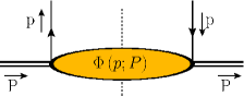
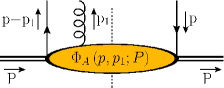
(a)                                                     (b)                                                (c)

Figure 1: The pictorial momentum space representation of the quark-quark correlator (a) and the quark-quark-gluon correlator for distribution functions (b) and a quark-quark correlator for fragmentation functions (c).

At high energies, the matrix elements appear as squared contributions in the correlators (including Dirac space indices $i$ and $j$),

$$\Phi_{ij}(p;P) = \sum_{X}\int\frac{d^{3}P_{X}}{(2\pi)^{3}\,2E_{X}}\ \langle P|\overline{\psi}_{j}(0)|X\rangle\,\langle X|\psi_{i}(0)|P\rangle\,\delta^{4}(p+P_{X}-P)$$ (1)

$$= \frac{1}{(2\pi)^{4}}\int d^{4}\xi\ e^{i\,p\cdot\xi}\ \langle P|\overline{\psi}_{j}(0)\,\psi_{i}(\xi)|P\rangle,$$

pictorially represented in Fig. 1(a). Usually, a summation over color indices is understood. This means that we will have $\Phi(p)={\rm Tr}_{c}\bigl{[}\Phi(p)\bigr{]}$, where $\Phi_{ij}(p)$ is considered to be also a matrix in color space, made explicit $\Phi_{ij;rs}\propto\psi_{ir}(\xi)\,\overline{\psi}_{js}(0)$. Including gluon fields one has quark-quark-gluon correlators like

$$\Phi^{\mu}_{A\,ij}(p,p_{1};P)=\frac{1}{(2\pi)^{8}}\int d^{4}\xi\,d^{4}\eta\ e^{i\,(p-p_{1})\cdot\xi}\ e^{i\,p_{1}\cdot\eta}\ \langle P|\overline{\psi}_{j}(0)\,A^{\mu}(\eta)\,\psi_{i}(\xi)|P\rangle,$$ (2)

illustrated in Fig. 1(b), and similarly matrix elements with more partons. The color structure of the field combination $\psi_{r}(\xi)\overline{\psi}_{s}(0)$ in the quark-quark-gluon correlator now actually has a color octet structure, with the simplest color trace being ${\rm Tr}_{c}[\psi\overline{\psi}A^{\mu}]$ if we write $A^{\mu}=A^{\mu a}T^{a}$ as a matrix-valued field. The corresponding correlators describing fragmentation into hadrons is for quarks given by

$$\Delta_{ij}(k;K_{h}) = \sum_{X}\frac{1}{(2\pi)^{4}}\int d^{4}\xi\ e^{-ik\cdot\xi}\,\langle 0|\psi_{i}(0)|K_{h},X\rangle\langle K_{h},X|\overline{\psi}_{j}(\xi)|0\rangle$$ (3)

$$= \frac{1}{(2\pi)^{4}}\int d^{4}\xi\ e^{-ik\cdot\xi}\,\langle 0|\psi_{i}(0)a_{h}^{\dagger}a_{h}\overline{\psi}_{j}(\xi)|0\rangle,$$

pictorially represented by the blob in Fig. 1(c). An averaging over color indices is implicit, thus $\Delta(k)=\frac{1}{N_{c}}{\rm Tr}_{c}\bigl{[}\Delta(k)\bigr{]}$ with again $\Delta(k)$ a diagonal matrix in color space. The second expression in the above involves hadronic creation and annihilation operators $a_{h}^{\dagger}|0\rangle=|K_{h}\rangle$.

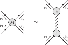
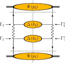
         (a)                                                         (b)

Figure 2: To illustrate the inclusion of correlators, we use the hard amplitude with one particular color flow for the quark lines as shown in (a). The squared amplitude needed for the cross section of the scattering process initiated by two hadrons is shown in (b).

The inclusion of the correlators in the description of a scattering process is similar to the inclusion of quark spinors or gluon polarizations. In the expression for the cross section of the (semi)-inclusive process $H_{1}(P_{1})+H_{2}(P_{2})\rightarrow h_{1}(K_{1})+h_{2}(K_{2})+\dots$ partonic momenta are approximately collinear, $P_{1}{\cdot}p_{1}\sim P_{2}{\cdot}p_{2}\sim K_{1}{\cdot}k_{1}\sim K_{2}{\cdot}k_{2}$ being of a hadronic mass scale, $M^{2}\sim 1$ GeV². This is to be compared to the usual hard invariants in the full or the partonic process such as $s\approx 2\,P_{1}{\cdot}P_{2}$, $t_{1}\approx-2\,K_{1}{\cdot}P_{1}$, $\hat{s}\approx 2\,p_{1}{\cdot}p_{2}$, $\hat{t}\approx-2\,k_{1}{\cdot}p_{1}$ (we will refer to this scale as the squared hard scale, $Q^{2}\gg M^{2}$).

The squared partonic amplitude $|\mathscr{M}|^{2}$ is convoluted with the correlators $\Phi(p,P)$ and $\Delta(k,K_{h})$. As illustrated in Figs 2(a) and (b) for an example in which (for simplicity) no color is exchanged in the hard process, the cross section is of the form

$$d\sigma\sim{\rm Tr}_{c}\bigl{[}\Phi(p_{1})\,\Gamma_{1}^{\ast}\,\Delta(k_{1})\,\Gamma_{1}\bigr{]}\,{\rm Tr}_{c}\bigl{[}\Phi(p_{2})\,\Gamma_{2}^{\ast}\,\Delta(k_{2})\,\Gamma_{2}\bigr{]},$$ (4)

where ${\rm Tr}_{c}\bigl{[}\ldots\bigr{]}$ parts are traced over color. In the case that the vertices $\Gamma$ don’t have any color structure, one can, because of the simple color singlet structure of $\Phi$ and $\Delta$ in the quark-quark correlators, perform the color trace separately for $\Phi$ and $\Delta$, ${\rm Tr}_{c}[\Phi(p)\,\Gamma^{\ast}\,\Delta(k)\,\Gamma]={\rm Tr}_{c}[\Phi(p)]\tfrac{1}{N_{c}}{\rm Tr_{c}}[\Delta(k)]\,\Gamma\,\Gamma^{\ast}$ (one summed and one averaged) and the cross section can be written in terms of the color-traced entities

$$d\sigma\sim\Phi(p_{1})\,\Phi(p_{2})\,\underbrace{\Gamma_{1}\,\Gamma_{1}^{\ast}\,\Gamma_{2}\,\Gamma_{2}^{\ast}}_{\hat{\Sigma}}\,\Delta(k_{1})\,\Delta(k_{2}),$$ (5)

where the remaining contractions are Dirac space and Lorentz indices, which have been suppressed in both Eqs 4 and 5. This expression still needs to be integrated over the parton momenta, which will be discussed next and of course should be extended with all possible correlators containing quark and gluon fields, in which cases color traces become more complicated.

The restriction to hard kinematics limits the number of diagrammatic contributions, although even at leading order, there still are many gluon contributions as will be discussed in Section 2. For parton momenta relevant in a hadron correlator we use the Sudakov decomposition,

$$p=x\,P+p_{\scriptscriptstyle T}+\underbrace{(p{\cdot}P-x\,M^{2})}_{\sigma}\,n,$$ (6)

where $n$ is a light-like vector $n$, satisfying $P{\cdot}n=1$ which can come from another hard (external) momenta, e.g. $n=P^{\prime}/P^{\prime}{\cdot}P$. The momentum fraction $x=p{\cdot}n=p^{n}$ is $\mathscr{O}(1)$. For any contractions with vectors outside the correlator $\Phi(p,P)$ one has $P\sim Q$, $p_{\scriptscriptstyle T}\sim M$ and $n\sim 1/Q$. Note that if $n$ is an exact light-like vector, one can construct two exact conjugate null-vectors, $n_{+}=P-\tfrac{1}{2}\,M^{2}\,n$ and $n_{-}=n$, satisfying $n_{+}{\cdot}n_{-}=1$ and $n_{+}^{2}=n_{-}^{2}=0$, that can be used to define light-cone components $a^{\pm}=a{\cdot}n_{\mp}$ (thus $x=p{\cdot}n_{-}=p^{+}$). Symmetric and antisymmetric ‘transverse’ projectors are defined as $g_{\scriptscriptstyle T}^{\mu\nu}=g^{\mu\nu}-n_{+}^{\{\mu}n_{-}^{\nu\}}$ and $\epsilon_{\scriptscriptstyle T}^{\mu\nu}=\epsilon^{n_{+}n_{-}\mu\nu}=\epsilon^{-+\mu\nu}=\epsilon^{Pn\mu\nu}$. In view of the relative importance of the components in this integration, one can, upon neglecting any $M^{2}/Q^{2}$ contributions in the cross section, integrate within a soft correlator over $p{\cdot}P$ (i.e. $p^{-}$) to obtain the TMD correlator

$$\Phi(x,p_{\scriptscriptstyle T};n)=\int d\,p{\cdot}P\ \Phi(p;P)=\left.\int\frac{d\,\xi{\cdot}P\,d^{2}\xi_{\scriptscriptstyle T}}{(2\pi)^{3}}\ e^{i\,p\cdot\xi}\ \langle P|\overline{\psi}(0)\,\psi(\xi)|P\rangle\right|_{LF}\ ,$$ (7)

which we will still consider as the unintegrated correlator. On the left-hand side the dependence on the hadron momentum $P$ has been suppressed. In the TMD correlator the nonlocality is restricted to the light-front (LF: $\xi{\cdot}n=\xi^{+}=0$) and the correlator depends on $x=p{\cdot}n$ and $p_{\scriptscriptstyle T}$. This light-front correlator is actually at equal (light-cone) time and time-ordering, thus, is automatic. This allows a direct interpretation of the correlator as a forward antiparton-hadron scattering amplitude, i.e. a Green function, untruncated in the parton legs [2]. This is the case for both collinear and TMD correlators [3]. This identification has been very important in deep inelastic processes [4], allowing the use of analyticity and unitarity properties of field theories, at least under the assumption that these properties apply to QCD. We will also need this later for fragmentation correlators.

Finally, the light-cone correlators are the collinear correlators containing the parton distribution functions depending only on the light-cone momentum fraction $x$, obtained upon integration over both $p{\cdot}P$ and $p_{\scriptscriptstyle T}$,

$$\Phi(x;n)=\int d\,p{\cdot}P\,d^{2}p_{\scriptscriptstyle T}\ \Phi(p;P)=\left.\int\frac{d\,\xi{\cdot}P}{(2\pi)}\ e^{i\,p\cdot\xi}\ \langle P|\overline{\psi}(0)\,\psi(\xi)|P\rangle\right|_{LC}\ ,$$ (8)

where the subscript LC refers to light-cone, implying $\xi{\cdot}n$ = $\xi_{\scriptscriptstyle T}$ = 0. This integration is generally allowed in hard processes up to $M^{2}/Q^{2}$ contributions and also up to contributions coming from the tails, e.g. logarithmically divergent contributions proportional to $\alpha_{s}(p_{\scriptscriptstyle T}^{2})/p_{\scriptscriptstyle T}^{2}$ tails [5]. The treatment of these in principle logarithmically divergent contributions require going beyond the tree-level resummation and consider next-to-leading order (NLO) QCD. In diagrammatic language these contributions involve ladder graphs describing the emission of gluons into the final state, relevant for the evolution of the correlators.

We end this section with a note on the measurability of the transverse momentum dependent (TMD) correlators. The collinear correlators are relevant in hard processes in which only hard scales (large invariants $\sim Q^{2}$ or ratios thereof, angles, rapidities) are measured. If one considers hadronic scale observables (transverse momenta within jets or slightly off-collinear configurations) one will need the TMD correlators for a full treatment. To identify the appropriate observable momentum for TMDs one must realize that the calculation of the cross section as schematically indicated in Eq. 4 involves momentum conservation at the partonic level, for instance $p+q=k$ for semi-inclusive deep inelastic scattering (DIS with $q$ being the space-like virtual photon momentum, $q^{2}=-Q^{2}$) or $p_{1}+p_{2}=k_{1}+k_{2}$ for a two-to-two process like the Drell-Yan process (DY where the final state is a lepton-pair with time-like momentum $q=k_{1}+k_{2}$ and $q^{2}=Q^{2}$).

Realizing that in the parametrization of partonic momenta, the momentum conservation can be used to identify the momentum fractions at high energies with scaling variables, e.g. for SIDIS one has for the fractions in the Sudakov expansions $p\approx xP+p_{\scriptscriptstyle T}$ and $k=K/z+k_{\scriptscriptstyle T}$

$$x\approx x_{B}\equiv\frac{Q^{2}}{2P{\cdot}q}\quad\mbox{and}\quad z\approx z_{h}\equiv\frac{P{\cdot}K}{P{\cdot}q},$$ (9)

equating $x$ to the Bjorken scaling variable and $z$ to the appropriate ratio of components of hadron momentum and photon momentum. Since these relations are correct up to $1/Q^{2}$ corrections, one finds that in the transverse directions one can identify

$$q_{\scriptscriptstyle T}\equiv q+x_{B}P-K/z_{h}=k_{\scriptscriptstyle T}-p_{\scriptscriptstyle T},$$ (10)

as the measurable transverse momentum up to order $1/Q$ corrections. Similarly for hadron initiated processes [6; 7; 8; 9] one can access transverse momenta. The best example is DY where one identifies the fractions with scaling variables

$$x_{1}=\frac{q{\cdot}P_{2}}{P_{1}{\cdot}P_{2}}\quad\mbox{and}\quad x_{2}=\frac{q{\cdot}P_{1}}{P_{2}{\cdot}P_{1}}$$ (11)

and finds that the relevant measure for transverse momentum is

$$q_{\scriptscriptstyle T}\equiv q-x_{1}P-x_{2}P_{2}=p_{1{\scriptscriptstyle T}}+p_{2{\scriptscriptstyle T}}.$$ (12)

In both cases one is left with a convolution of the partonic transverse momenta in the hadrons. One can extend this to off-collinearity of jets or produced hadrons in the final state in more complicated hadron-hadron scattering processes.

2 Color gauge invariance

The correlators encompass the information on the soft parts. They depend on the hadron and quark momenta $P$ and $p$ (and in general also spin vectors). Depending on the Lorentz and Dirac structure of the matrix elements involved one can look for the pieces in the correlator that show up as the most dominant matrix elements among the contributions in the hard process. These are those that have the maximum number of contractions with $n$, which minimizes the powers of $M$ that after contraction of open indices inevitably is the scale of the hadronic matrix elements. Including also gluon fields, they are

$$\langle\ \overline{\psi}(0)\hbox to0.0pt{\hbox to6.00235pt{\hfil/\hfil}\hss}n\psi(\xi)\ \rangle\qquad\mbox{and}\qquad\langle\ G^{n\alpha}(0)G^{n\beta}(\xi)\ \rangle,$$ (13)

(the latter with transverse indices $\alpha$ and $\beta$). The two matrix elements above have canonical dimension two. The corresponding local matrix elements, $\overline{\psi}(0)\,\hbox to0.0pt{\hbox to6.00235pt{\hfil/\hfil}\hss}n\,\psi(0)$ and $G^{n\alpha}(0)\,G^{n\beta}(0)$ for quarks and gluons, respectively, are color-gauge-invariant (twist two) operators. The nonlocal combinations in Eq. 13, however, are not gauge-invariant. Expanded into local operators, the expansion would involve operator combinations with derivatives such as $\overline{\psi}(0)\,\hbox to0.0pt{\hbox to6.00235pt{\hfil/\hfil}\hss}n\,\partial^{n}\ldots\partial^{n}\,\psi(0)$. Color gauge invariance in the correlators requires in the local matrix elements covariant derivatives or in the nonlocal matrix elements the presence of a gauge link connecting the two fields. For the light-cone correlators the gauge link corresponds to the inclusion of an arbitrary number of ‘leading’ gluon fields $A^{n}(\eta)$ in the field combinations in Eq. 13 which are resummed into a gauge link $\overline{\psi}(0)\,U^{[n]}_{[0,\xi]}\,\psi(\xi)$ = ${\rm Tr}_{c}\bigl{[}U^{[n]}_{[0,\xi]}\,\psi(\xi)\overline{\psi}(0)\bigr{]}$, given by

$$U^{[n]}_{[0,\xi]}={\mathscr{P}}\,\exp\left(-i\int_{0}^{\xi}d\,\eta{\cdot}P\ n{\cdot}A(\eta)\right).$$ (14)

Including this gauge link, the nonlocal operator combinations

$$\left.\langle\ \overline{\psi}(0)\hbox to0.0pt{\hbox to6.00235pt{\hfil/\hfil}\hss}n\,U^{[n]}_{[0,\xi]}\psi(\xi)\ \rangle\right|_{LC}\qquad\mbox{and}\qquad\left.\langle\ G^{n\alpha}(0)\,U^{[n]}_{[0,\xi]}G^{n\beta}(\xi)\,U^{[n]}_{[\xi,0]}\ \rangle\right|_{LC}$$ (15)

can be expanded into twist two operators $\overline{\psi}(0)\,\hbox to0.0pt{\hbox to6.00235pt{\hfil/\hfil}\hss}n\,D^{n}\ldots D^{n}\,\psi(0)$ and $G^{n\alpha}(0)\,D^{n}\ldots D^{n}\,G^{n\beta}(0)$ for quarks and gluons, respectively (number of $D^{n}$’s is the spin of these operators). Also TMD correlators require a gauge link, but the separation of the two fields is no longer a simple light-like one and they involve derivatives with transverse indices. It is important to realize that in principle any gauge link with an arbitrary path gives a gauge-invariant combination. What is the appropriate link contributing at leading order (in $M/Q$) in a given hard scattering process, however, is calculable [10].

The calculation involves diagrams with additional gluon fields in the correlator. The important ones at leading order are the $A^{n}$ gluons which do not increase the canonical dimension and hence also appear at leading order. Couplings of these gluons into the hard part cancel using Ward identities and the couplings to the external lines (see Fig. 3) produce a Wilson line running from the positions $0$ or $\xi$ in the parton fields to $\xi^{-}=\pm\infty$ depending on the external line being an incoming parton or outgoing parton.

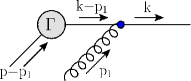
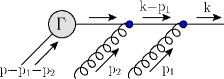
$A_{0}$                                                $A_{1}$                                            $A_{2}$

Figure 3: Inclusion of collinear gluons from $\Phi_{A\ldots A}(p-p_{1}\ldots-p_{N},p_{1},\ldots,p_{N})$ coupling to an outgoing (colored) quark line with momentum $k$. These insertions give rise to the gauge link $U_{+}^{[k]}[p]$ in Eq. 16.

(a)                (b)     

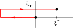
Figure 4: The staple-like gauge link structure in the quark-quark correlator $\Phi$ in SIDIS (a) and DY (b) respectively.

We note that the gauge link also involves transverse gluons showing that in processes involving more hadrons the effects of transverse gluons are not necessarily suppressed. Integration over transverse momenta implies in the correlator, which is a Fourier transform, that $\xi_{\scriptscriptstyle T}=0_{\scriptscriptstyle T}$, in which case the $U^{[+]}$ and $U^{[-]}$ links reduce to a unique collinear link connecting $0$ and $\xi^{-}$. Technically, the transverse gluons emerge as boundary terms at light-cone infinity [11; 12] that are needed to rewrite transverse gluon fields $A^{\alpha}$ into field strengths $G^{n\alpha}$. Physically they can also be seen to correspond to soft gluons as shown in explicit model calculations [13; 14]. If only one hadron appears in the high-energy scattering process, this produces the color-gauge-invariant matrix elements with for transverse momentum dependent correlators (cf. Eq. 7) as simplest gauge links the ones shown in Fig. 4 for quark correlators and in Fig. 5 for gluon correlators. For collinear correlators (cf. Eq. 8) the staple-like gauge links reduce to a unique straight-line gauge link with single or double color lines for quarks or gluons respectively.

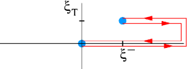
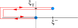
(a)                                                      (b)

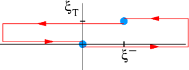
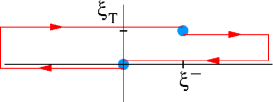
(c)                                                      (d)

Figure 5: The gauge links for gluon TMDs. We note that for gluons the double color line may ‘split’ in the hard part and connect to an initial state and a final state parton giving rise to the gauge link structures in (c) and (d).

3 Color entanglement

The color structure of various correlators becomes entangled if the color flow is more complicated [10; 15; 16; 17; 18; 19]. Following again Ref. [1] we find for the gluon insertions coming from a particular correlator and coupling to an outgoing fermion line a Wilson line connecting to light-cone $+\infty$. E.g. the gauge link $U_{+}^{[k_{1}]}[p_{1}]$ emerges from diagrams as shown in Fig. 3. Including all multi-gluon interactions originating from $\Phi(p_{1})$ in Fig. 2(b) and transverse pieces, we get the result

$$d\sigma \sim {\rm Tr}_{c}\bigl{[}\Phi(p_{1})\,\Gamma_{1}^{\ast}\,U_{+}^{[k_{1}]\dagger}[p_{1}]\Delta(k_{1})U_{+}^{[k_{1}]}[p_{1}]\,\Gamma_{1}\bigr{]}$$ (16)

$$\mbox{}\times{\rm Tr}_{c}\bigl{[}U_{-}^{[p_{2}]\dagger}[p_{1}]\,\Phi(p_{2})\,U_{-}^{[p_{2}]}[p_{1}]\,\Gamma_{2}^{\ast}\,U_{+}^{[k_{2}]\dagger}[p_{1}]\,\Delta(k_{2})\,U_{+}^{[k_{2}]}[p_{1}]\,\Gamma_{2}\bigr{]},$$

in which the (color charge of the) Wilson line is stuck in the color traces at the ‘positions’ corresponding to the external parton lines. Although the light-like directions in the gauge links involve different light-like directions, these are all ‘orthogonal’ light-like directions to $p_{1}$ and can at leading order simply be replaced by a single generic null-vector $n$.

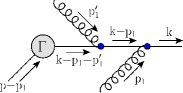
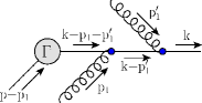
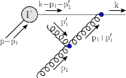
(a)                                            (b)                                            (c)

Figure 6: The gluon insertions on an outgoing quark line coming from two different soft pieces, one from $\Phi(p)$ and one from $\Phi(p^{\prime})$, respectively.

Including gluon insertions from several correlators, for instance those on an outgoing quark line coming from two different soft pieces, one from $\Phi(p)$ and one from $\Phi(p^{\prime})$, such as given in Fig. 6, gives rise to intertwined Wilson lines illustrated in Fig. 7.

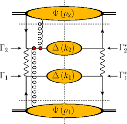
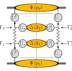
(a)                                            (b)                                             (c)

Figure 7: (a) An example of a diagram with two gluons attaching to the same outgoing line with momentum $k_{2}$. (b) They result into one gauge connection $U^{[k_{2}]}_{+}[p_{1},p_{2},k_{1}]$, which combines all collinear gluons coming from $\Phi(p_{1})$, $\Phi(p_{2})$ and $\Delta(k_{1})$. (c) Gauge connections appear on all external (colored) lines.

Including all multi-gluon interactions as well as the corresponding transverse pieces from $\Phi(p_{1})$, $\Delta(k_{1})$, $\Phi(p_{2})$ and $\Delta(k_{2})$ onto all legs, Eq. 16 generalizes to

$$d\sigma \sim {\rm Tr}_{c}\bigl{[}U_{-}^{[n]\dagger}[p_{2},k_{1},k_{2}]\,\Phi(p_{1})\,U_{-}^{[n]}[p_{2},k_{1},k_{2}]\,\Gamma_{1}^{\ast}\,U_{+}^{[n]\dagger}[p_{1},p_{2},k_{2}]\Delta(k_{1})\,U_{+}^{[n]}[p_{1},p_{2},k_{2}]\,\Gamma_{1}\bigr{]}$$ (17)

$$\mbox{}\times{\rm Tr}_{c}\bigl{[}U_{-}^{[n]\dagger}[p_{1},k_{1},k_{2}]\,\Phi(p_{2})\,U_{-}^{[n]}[p_{1},k_{1},k_{2}]\,\Gamma_{2}^{\ast}\,U_{+}^{[n]\dagger}[p_{1},p_{2},k_{1}]\,\Delta(k_{2})\,U_{+}^{[n]}[p_{1},p_{2},k_{1}]\,\Gamma_{2}\bigr{]},$$

illustrated in Fig. 8. The result for all insertions to a particular leg is a color symmetric combination of the insertions from all correlators,

$$U_{+}^{[n]}[p_{1},p_{2},k_{1}]={\mathcal{S}}\{U_{+}^{[n]}[p_{1}]U_{+}^{[n]}[p_{2}]U_{+}^{[n]}[k_{1}]\},$$ (18)

in which the full symmetrization makes the ordering of the three connections on the right-hand side irrelevant.

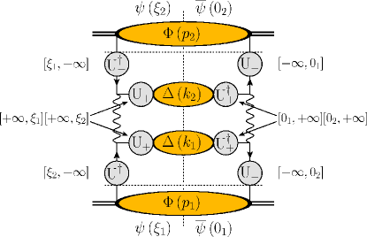
(a)                                                (b)

Figure 8: (a) We have indicated for the correlators and gauge connections also the actual space-time points they are bridging, limiting ourselves for simplicity to the coordinates conjugate to $p_{1}$ (points $0_{1}$ and $\xi_{1}$; see also the discussion following Eq. 16) and $p_{2}$ (points $0_{2}$ and $\xi_{2}$), leaving out the space-time structure for the fragmentation correlators for which we would have to include also the coordinates conjugate to $k_{1}$ and $k_{2}$. (b) Shown are some combinations of the gauge links including transverse pieces that can show up in the correlators. These can be Wilson lines and Wilson loops

The resulting expression in Eq. 17 is now color-gauge-invariant. The Wilson lines can be taken along a generic $n$-direction, but its color structure is fully entangled and it does not allow for a factorized expression with universal correlators that have their own gauge links. Viewing it as a factorized expression it contains hard amplitudes, soft correlators and gauge connections, where the gauge connections take care of a ‘color resetting’, which feels all hadrons that are involved.

If one is interested in an expression for the cross section integrated over transverse momenta, one can combine the Wilson lines to and from light-cone $\pm\infty$, now all made up of $A^{n}$ fields, into finite straight-line Wilson lines, $U_{+}^{[n]\dagger}[p_{1}]\,U_{+}^{[n]}[p_{1}]$, since after the integration over $p_{1{\scriptscriptstyle T}}$ they not only both run along $n$, but they coincide since one also has $0_{\scriptscriptstyle T}=\xi_{\scriptscriptstyle T}$. Furthermore, it is irrelevant if one started from Wilson lines running via plus or via minus infinity, and also the direction $n$ is in fact irrelevant, being just the direction of the straight line connecting $0$ and $\xi$. We recall that the argument $p_{1}$ or $x_{1}$, given to the Wilson lines, is simply needed to indicate that the fields in that Wilson line belong to the correlator $\Phi(x_{1})$, which is the Fourier transform of the matrix element $\langle\overline{\psi}(0)\psi(\xi)\rangle$. Thus, in coordinate space one just has the Wilson line in Eq. 14, which connects the points $0$ and $\xi$ in $\Phi(x_{1})$ composed of two pieces. As far as relevant for $\Phi(x_{1})$, the Wilson lines in the first trace form a gauge link, those in the second trace form a closed loop, which in the collinear situation (when $0_{\scriptscriptstyle T}=\xi_{\scriptscriptstyle T}$) becomes a unit operator in color space. One is left with

$$\sigma \sim {\rm Tr}_{c}\bigl{[}U_{-}^{[n]\dagger}[k_{1}]\,\Phi(x_{1})\,U_{-}^{[n]}[k_{1}]\,\Gamma_{1}^{\ast}\,U_{-}^{[n]\dagger}[p_{1}]\Delta(z_{1})\,U_{-}^{[n]}[p_{1}]\bigr{]}$$ (19)

$$\mbox{}\times\,{\rm Tr}_{c}\bigl{[}U_{-}^{[n]\dagger}[k_{2}]\,\Phi(x_{2})\,U_{-}^{[n]}[k_{2}]\,\Gamma_{2}^{\ast}\,U_{-}^{[n]\dagger}[p_{2}]\,\Delta(z_{2})\,U_{-}^{[n]}[p_{2}]\,\Gamma_{2}\bigr{]}.$$

The way of turning the gauge connections into gauge links at the collinear stage is actually just applying gauge transformations $U^{[n]}_{[a,\xi]}$ (with a fixed point $a$) to all fields and using the fact that they in the collinear case only involve fields $A^{n}$. One obtains

$$\sigma\sim\Phi^{[U]}(x_{1})\Phi^{[U]}(x_{2})\,\underbrace{\Gamma_{1}\,\Gamma_{1}^{\ast}\,\Gamma_{2}\,\Gamma_{2}^{\ast}}_{\hat{\Sigma}}\,\Delta^{[U]}(z_{1})\,\Delta^{[U]}(z_{2}),$$ (20)

where

$$\Phi^{[U]}(x) = {\rm Tr}_{c}\bigl{[}U_{\pm}^{[n]}[p]\Phi(x)\,U_{\pm}^{[n]\dagger}[p]\bigr{]}=\left.\int\frac{d\,\xi{\cdot}P}{2\pi}\ e^{i\,p\cdot\xi}\ \langle P|\overline{\psi}(0)\,U_{[0,\pm\infty]}^{[n]}\,U_{[\pm\infty,\xi]}^{[n]}\,\psi(\xi)|P\rangle\right|_{LC}$$ (21)

$$= {\rm Tr}_{c}\bigl{[}U^{[n]}[p]\,\Phi(x)\bigr{]}=\left.\int\frac{d\,\xi{\cdot}P}{2\pi}\ e^{i\,p\cdot\xi}\ \langle P|\overline{\psi}(0)\,U^{[n]}_{[0,\xi]}\,\psi(\xi)|P\rangle\right|_{LC}$$

and

$$\Delta^{[U]}(z) = \frac{1}{N_{c}}\,{\rm Tr}_{c}\bigl{[}U_{\pm}^{[n]}[k]\Delta(z)\,U_{\pm}^{[n]\dagger}[k]\bigr{]}=\frac{1}{N_{c}}\,{\rm Tr}_{c}\bigl{[}\Delta(z)\,U^{[n]\dagger}[k]\bigr{]}$$ (22)

$$= \left.\int\frac{d\,\xi{\cdot}K_{h}}{2\pi}\ e^{-ik\cdot\xi}\,\frac{1}{N_{c}}\,{\rm Tr}_{c}\langle 0|U_{[\pm\infty,0]}^{[n]}\psi(0)a_{h}^{\dagger}a_{h}\overline{\psi}(\xi)\,U_{[\xi,\pm\infty]}^{[n]}|0\rangle\right|_{LC}$$

are the color-gauge-invariant collinear correlators, including unique gauge links along the light-like separation. The gauge link being unique, it is usually omitted, writing $\Phi(x_{1})$, $\Phi(x_{2})$, $\Delta(z_{1})$ and $\Delta(z_{2})$. These (color-gauge-invariant) correlators can be expanded in terms of the standard unpolarized and polarized parton distribution functions and fragmentation functions, respectively.

Finally, if the transverse momentum in all correlators except one, say $\Phi(p_{1})$, is integrated over, one can shuffle all gauge links into the respective correlators. We refer to these processes as 1-parton unintegrated processes [1]. All gauge links only involve collinear fields $A^{n}$ and are straight-line Wilson lines, except for the gauge link belonging to $\Phi(p_{1})$, for which the transverse separations are relevant. In simple processes like SIDIS and DY the longitudinal and transverse pieces in the remaining TMD correlator then combine into the staple-like gauge links in Fig. 4. The gauge link for $\Phi(p_{1})$ in the case of a process in which the color flow is more complicated, such as in the example shown in Fig. 2(b), involves a more complex path, such as $U^{[+]}_{[0,\xi]}\,\operatorname{Tr}_{c}(U^{[\Box]})$, in which a staple-like link is combined with a Wilson loop $U^{\Box}$ = $U^{[+]}_{[0,\xi]}\,U^{[-]}_{[\xi,0]}$ (see also Fig. 8(b)). The particular TMD correlator $\Phi^{[U]}(x_{1},p_{1{\scriptscriptstyle T}})$ is color-gauge-invariant and can be expanded in terms of parton distribution functions depending on $x$ and $p_{\scriptscriptstyle T}^{2}$, although these would in principle still be gauge link-dependent, for instance for quarks [20; 21],

$$\Phi^{[U]}(x,p_{{\scriptscriptstyle T}};n) = \bigg{\{}f^{[U]}_{1}(x,p_{\scriptscriptstyle T}^{2})-f_{1T}^{\perp[U]}(x,p_{\scriptscriptstyle T}^{2})\,\frac{\epsilon_{{\scriptscriptstyle T}}^{\rho\sigma}p_{{\scriptscriptstyle T}\rho}S_{{\scriptscriptstyle T}\sigma}}{M}+g^{[U]}_{1s}(x,p_{\scriptscriptstyle T})\gamma_{5}$$ (23)

$$\mbox{}+h^{[U]}_{1T}(x,p_{\scriptscriptstyle T}^{2})\,\gamma_{5}\,\hbox to0.0pt{\hbox to6.70831pt{\hfil/\hfil}\hss}S_{{\scriptscriptstyle T}}+h_{1s}^{\perp[U]}(x,p_{\scriptscriptstyle T})\,\frac{\gamma_{5}\,\hbox to0.0pt{\hbox to5.03125pt{\hfil/\hfil}\hss}p_{{\scriptscriptstyle T}}}{M}+ih_{1}^{\perp[U]}(x,p_{\scriptscriptstyle T}^{2})\,\frac{\hbox to0.0pt{\hbox to5.03125pt{\hfil/\hfil}\hss}p_{{\scriptscriptstyle T}}}{M}\bigg{\}}\frac{\hbox to0.0pt{\hbox to7.80904pt{\hfil/\hfil}\hss}P}{2},$$

with the spin vector parametrized as $S^{\mu}=S_{{\scriptscriptstyle L}}P^{\mu}+S^{\mu}_{{\scriptscriptstyle T}}+M^{2}\,S_{{\scriptscriptstyle L}}n^{\mu}$ and shorthand notations for $g^{[U]}_{1s}$ and $h_{1s}^{\perp[U]}$,

$$g^{[U]}_{1s}(x,p_{T})=S_{{\scriptscriptstyle L}}g^{[U]}_{1L}(x,p_{{\scriptscriptstyle T}}^{2})-\frac{p_{{\scriptscriptstyle T}}\cdot S_{{\scriptscriptstyle T}}}{M}g^{[U]}_{1T}(x,p_{{\scriptscriptstyle T}}^{2}).$$ (24)

4 TMDs of definite rank

Integrating over components of the parton momenta in the correlators one goes from TMDs to collinear correlators and finally to local matrix elements. Including moments in these integrations is a way to obtain the coefficients in an expansion, e.g. the way that local matrix elements play a role in the operator product expansion. The behavior of the local matrix elements, characterized by spin and twist, are useful in determining the relevance at leading or subleading orders. To study the $x$-dependence of the integrated correlator $\Phi(x)$ one constructs the $x^{N}$ moments. To relate these to local matrix elements, the Wilson lines are essential since by taking moments in $x$ one needs derivatives in $\xi^{-}$,

$$x^{N}\Phi^{[U]}(x) = \left.\int\frac{d\,\xi{\cdot}P}{2\pi}\ e^{i\,p{\cdot}\xi}\ \langle P|\overline{\psi}(0)\,(i\partial^{n})^{N}\,U^{n}_{[0,\xi]}\,\psi(\xi)|P\rangle\right|_{LC}$$ (25)

$$= \left.\int\frac{d\,\xi{\cdot}P}{2\pi}\ e^{i\,p{\cdot}\xi}\ \langle P|\overline{\psi}(0)\,U^{n}_{[0,\xi]}\,(iD^{n})^{N}\,\psi(\xi)|P\rangle\right|_{LC}.$$

Integrating over $x$ one finds the connection of the Mellin moments of PDFs involving covariant derivatives $D^{n}$ as has been already discussed following Eq. 13. The local matrix elements have specific anomalous dimensions, which via an inverse Mellin transform define the splitting functions.

For transverse momentum dependence, we want to expand the TMD correlators as

$$\Phi(x,p_{\scriptscriptstyle T})=\sum_{m}\Phi^{(m)}(x,p_{\scriptscriptstyle T}^{2})\,p_{\scriptscriptstyle T}^{m}(\varphi),$$ (26)

where the angle $\varphi$ represents the angular dependence of the transverse vectors $p_{\scriptscriptstyle T}$ and $p_{\scriptscriptstyle T}^{m}(\varphi)$ is the symmetric traceless rank $m$ tensor constructed from the transverse momenta, i.e.

$$p_{\scriptscriptstyle T}^{\alpha_{1}\ldots\alpha_{m}}=p_{\scriptscriptstyle T}^{\alpha_{1}}\ldots p_{\scriptscriptstyle T}^{\alpha_{m}}-{\rm traces}\ \Longleftrightarrow\ p_{\scriptscriptstyle T}^{m}(\varphi)=\frac{|p_{\scriptscriptstyle T}|^{m}}{2^{m-1}}\,e^{\pm im\varphi}.$$ (27)

To find the coefficients in such an expansion, we use transverse moments that involve $p_{\scriptscriptstyle T}$-weightings of the light-front TMD in Eq. (7), including now also a gauge link $U$. For the simplest gauge links $U^{[\pm]}$, one has

$$p_{\scriptscriptstyle T}^{\alpha}\,\Phi^{[\pm]}(x,p_{\scriptscriptstyle T};n) = \int\frac{d\,\xi{\cdot}P\,d^{2}\xi_{\scriptscriptstyle T}}{(2\pi)^{3}}\ e^{i\,p{\cdot}\xi}$$ (28)

$$\mbox{}\times\langle P|\overline{\psi}(0)\,U^{n}_{[0,\pm\infty]}\,U^{T}_{[0_{\scriptscriptstyle T},\xi_{\scriptscriptstyle T}]}\,iD_{\scriptscriptstyle T}^{\alpha}(\pm\infty)\,U^{n}_{[\pm\infty,\xi]}\psi(\xi)|P\rangle\Biggr{|}_{LF}.$$

Integrating over $p_{\scriptscriptstyle T}$ gives the lowest transverse moment. This moment involves twist three (or higher) collinear multi-parton correlators, in particular the quark-quark-gluon correlator

$$\Phi^{n\alpha}_{F}(x-x_{1},x_{1}|x) = \int\frac{d\,\xi{\cdot}P\,d\,\eta{\cdot}P}{(2\pi)^{2}}\ e^{i\,(p-p_{1}){\cdot}\xi}\$$ (29)

$$\mbox{}\hskip 14.22636pt\times e^{i\,p_{1}{\cdot}\eta}\ \langle P|\overline{\psi}(0)\,U^{n}_{[0,\eta]}\,F^{n\alpha}(\eta)\,U^{n}_{[\eta,\xi]}\,\psi(\xi)|P\rangle\Biggr{|}_{LC}.$$

In terms of this correlator and the similarly defined correlator $\Phi_{D}^{\alpha}(x-x_{1},x_{1}|x)$ one finds

$$\int d^{2}p_{\scriptscriptstyle T}\ p_{\scriptscriptstyle T}^{\alpha}\,\Phi^{[U]}(x,p_{\scriptscriptstyle T})=\widetilde{\Phi}_{\partial}^{\alpha}(x)+C_{G}^{[U]}\,\Phi_{G}^{\alpha}(x),$$ (30)

with

$$\widetilde{\Phi}_{\partial}^{\alpha}(x) = \Phi_{D}^{\alpha}(x)-\Phi_{A}^{\alpha}(x)$$ (31)

$$= \int dx_{1}\,\Phi_{D}^{\alpha}(x-x_{1},x_{1}|x)-\int dx_{1}\,\text{PV}\frac{1}{x_{1}}\,\Phi_{F}^{n\alpha}(x-x_{1},x_{1}|x),$$

$$\Phi_{G}^{\alpha}(x) = \pi\Phi_{F}^{n\alpha}(x,0|x).$$ (32)

The latter is referred to as a gluonic pole or ETQS-matrix element [22; 23; 24; 25; 26; 27]. The function $\Phi_{G}^{\alpha}(x)$ is a gluonic pole matrix element, corresponding to the emission of a collinear gluon of zero momentum [13; 14]. These functions are collinear and independent of the gauge link. That dependence is only in the gluonic pole coefficient $C_{G}^{[U]}$. For the simple staple gauge links $U_{\pm}$ the gluonic pole coefficients are $C_{G}^{[\pm]}=\pm 1$. An important property of the two functions showing up in the moments, is their behavior under time-reversal. While $\widetilde{\Phi}_{\partial}^{\alpha}$ is T-even, $\Phi_{G}^{\alpha}$ is T-odd. Since time-reversal is a good symmetry of QCD, the appearance of T-even or T-odd functions in the parametrization of the correlators is linked to specific observables with this same character. In particular single spin asymmetries are T-odd observables.

Similarly, we have higher moments,

$$\Phi_{\partial\partial}^{\alpha\beta\,[U]}(x)=\widetilde{\Phi}_{\partial\partial}^{\alpha\beta}(x)+C_{G}^{[U]}\,\widetilde{\Phi}_{\{\partial G\}}^{\alpha\beta}(x)+C_{GG,c}^{[U]}\,\Phi_{GG,c}^{\alpha\beta}(x),$$ (33)

etc. An extra index $c$ is needed if there are multiple possibilities to construct a color singlet as is the case for a field combination $\overline{\psi}\,GG\,\psi$, namely $\operatorname{Tr}_{c}[GG\psi\overline{\psi}]$ ($c=1$) and $\operatorname{Tr}_{c}[GG]\,\operatorname{Tr}_{c}[\psi\overline{\psi}]/N_{c}$ ($c=2$). The number of gluonic poles determines if we have a T-even or T-odd operator combination. With two color possibilities for a double gluonic pole, there are thus three rank two T-even operator structures, which in the parametrization of the correlator will imply three different pretzelocity functions. For the staple-like links only one configuration is relevant, having $C_{GG,1}^{[\pm]}=1$ and $C_{GG,2}^{[\pm]}=0$. The weighted results also allow a unique parametrization of the gauge link dependent TMD correlators in terms of a finite set of definite rank TMDs depending on $x$ and $p_{\scriptscriptstyle T}^{2}$, azimuthal tensors and gluonic pole factors [28; 29],

$$\Phi^{[U]}(x,p_{\scriptscriptstyle T}) = \Phi(x,p_{\scriptscriptstyle T}^{2})+\frac{p_{{\scriptscriptstyle T}i}}{M}\,\widetilde{\Phi}_{\partial}^{i}(x,p_{\scriptscriptstyle T}^{2})+\frac{p_{{\scriptscriptstyle T}ij}}{M^{2}}\,\widetilde{\Phi}_{\partial\partial}^{ij}(x,p_{\scriptscriptstyle T}^{2})$$ (34)

$$\mbox{}+C_{G}^{[U]}\left\lgroup\frac{p_{{\scriptscriptstyle T}i}}{M}\,\Phi_{G}^{i}(x,p_{\scriptscriptstyle T}^{2})+\frac{p_{{\scriptscriptstyle T}ij}}{M^{2}}\,\widetilde{\Phi}_{\{\partial G\}}^{\,ij}(x,p_{\scriptscriptstyle T}^{2})\right\rgroup$$

$$\mbox{}+\sum_{c}C_{GG,c}^{[U]}\frac{p_{{\scriptscriptstyle T}ij}}{M^{2}}\,\Gamma_{GG,c}^{ij}(x,p_{\scriptscriptstyle T}^{2}).$$

Depending on partons (quarks or gluons) and target, there is a maximum rank, which for quarks in a nucleon is rank 2. For gluons in a nucleon one has to go up to rank 3. Actually for the highest rank, time-reversal symmetry does not allow a time-reversal odd rank 2 correlator, i.e. $\widetilde{\Phi}_{\{\partial G\}}=0$. Note that since the tensors $p_{\scriptscriptstyle T}^{ij}$ on the rhs of Eq. 34 are traceless and symmetric, the correlators they multiply also must be made traceless in order to make the identification of the correlators unique.

The situation with universality for fragmentation functions is easier because the gluonic pole matrix elements vanish in that case [30; 31; 32; 33]. Nevertheless, there exist T-odd fragmentation functions, but their QCD operator structure is T-even. These T-odd functions then appear in the parametrization of $\widetilde{\Phi}_{\partial}^{\alpha}$. Hence, there is no process dependence from gluonic pole factors for fragmentation functions.

The reproduction of the transverse moments provides the proper identification of universal TMD functions, e.g. for quarks

$$\Phi(x,p_{\scriptscriptstyle T}^{2})=\bigg{\{}f_{1}(x,p_{\scriptscriptstyle T}^{2})+S_{{\scriptscriptstyle L}}\,g_{1}(x,p_{\scriptscriptstyle T}^{2})\gamma_{5}+h_{1}(x,p_{\scriptscriptstyle T}^{2})\gamma_{5}\,\hbox to0.0pt{\hbox to6.70831pt{\hfil/\hfil}\hss}S_{{\scriptscriptstyle T}}\bigg{\}}\frac{\hbox to0.0pt{\hbox to7.80904pt{\hfil/\hfil}\hss}P}{2},$$ (35)

$$\frac{p_{{\scriptscriptstyle T}i}}{M}\,\widetilde{\Phi}_{\partial}^{i}(x,p_{\scriptscriptstyle T}^{2})=\bigg{\{}h_{1L}^{\perp}(x,p_{\scriptscriptstyle T}^{2})\,S_{{\scriptscriptstyle L}}\frac{\gamma_{5}\,\hbox to0.0pt{\hbox to5.03125pt{\hfil/\hfil}\hss}p_{{\scriptscriptstyle T}}}{M}-g_{1T}(x,p_{\scriptscriptstyle T}^{2})\,\frac{p_{\scriptscriptstyle T}{\cdot}S_{\scriptscriptstyle T}}{M}\gamma_{5}\bigg{\}}\frac{\hbox to0.0pt{\hbox to7.80904pt{\hfil/\hfil}\hss}P}{2},$$ (36)

$$\frac{p_{{\scriptscriptstyle T}i}}{M}\,\Phi_{G}^{i}(x,p_{\scriptscriptstyle T}^{2})=\bigg{\{}-f_{1T}^{\perp}(x,p_{\scriptscriptstyle T}^{2})\,\frac{\epsilon_{{\scriptscriptstyle T}}^{\rho\sigma}p_{{\scriptscriptstyle T}\rho}S_{{\scriptscriptstyle T}\sigma}}{M}+ih_{1}^{\perp}(x,p_{\scriptscriptstyle T}^{2})\,\frac{\hbox to0.0pt{\hbox to5.03125pt{\hfil/\hfil}\hss}p_{{\scriptscriptstyle T}}}{M}\bigg{\}}\frac{\hbox to0.0pt{\hbox to7.80904pt{\hfil/\hfil}\hss}P}{2},$$ (37)

$$\frac{p_{{\scriptscriptstyle T}ij}}{M^{2}}\widetilde{\Phi}_{\partial\partial}^{ij}(x,p_{\scriptscriptstyle T}^{2})=h_{1T}^{\perp(A)}(x,p_{\scriptscriptstyle T}^{2})\,\frac{p_{{\scriptscriptstyle T}ij}S_{\scriptscriptstyle T}^{i}\,\gamma_{5}\gamma_{{\scriptscriptstyle T}}^{j}}{M^{2}}\,\frac{\hbox to0.0pt{\hbox to7.80904pt{\hfil/\hfil}\hss}P}{2},$$ (38)

$$\frac{p_{{\scriptscriptstyle T}ij}}{M^{2}}\Phi_{GG,1}^{ij}(x,p_{\scriptscriptstyle T}^{2})=h_{1T}^{\perp(B1)}(x,p_{\scriptscriptstyle T}^{2})\,\frac{p_{{\scriptscriptstyle T}ij}S_{\scriptscriptstyle T}^{i}\,\gamma_{5}\gamma_{{\scriptscriptstyle T}}^{j}}{M^{2}}\,\frac{\hbox to0.0pt{\hbox to7.80904pt{\hfil/\hfil}\hss}P}{2},$$ (39)

$$\frac{p_{{\scriptscriptstyle T}ij}}{M^{2}}\Phi_{GG,2}^{ij}(x,p_{\scriptscriptstyle T}^{2})=h_{1T}^{\perp(B2)}(x,p_{\scriptscriptstyle T}^{2})\,\frac{p_{{\scriptscriptstyle T}ij}S_{\scriptscriptstyle T}^{i}\,\gamma_{5}\gamma_{{\scriptscriptstyle T}}^{j}}{M^{2}}\,\frac{\hbox to0.0pt{\hbox to7.80904pt{\hfil/\hfil}\hss}P}{2},$$ (40)

$$\frac{p_{{\scriptscriptstyle T}ij}}{M^{2}}\widetilde{\Phi}_{\{\partial G\}}^{ij}(x,p_{\scriptscriptstyle T}^{2})=0.$$ (41)

We note that the rank zero functions in Eq. (35) depend on $x$ and $p_{\scriptscriptstyle T}^{2}$ and involve traces, to be precise $g_{1}(x,p_{\scriptscriptstyle T}^{2})=g_{1L}^{[U]}(x,p_{\scriptscriptstyle T}^{2})$ and $h_{1}(x,p_{\scriptscriptstyle T}^{2})=h_{1T}^{[U]}(x,p_{\scriptscriptstyle T}^{2})-(p_{\scriptscriptstyle T}^{2}/2M^{2})\,h_{1T}^{\perp[U]}(x,p_{\scriptscriptstyle T}^{2})$. As remarked before, for the pretzelocity there are three universal functions with in general

$$h_{1T}^{\perp[U]}(x,p_{\scriptscriptstyle T}^{2})=h_{1T}^{\perp(A)}(x,p_{\scriptscriptstyle T}^{2})+C_{GG,1}^{[U]}\,h_{1T}^{\perp(B1)}(x,p_{\scriptscriptstyle T}^{2})+C_{GG,2}^{[U]}\,h_{1T}^{\perp(B2)}(x,p_{\scriptscriptstyle T}^{2}).$$ (42)

For the simplest gauge links we have $C_{GG,1}^{[\pm]}=1$ and $C_{GG,2}^{[\pm]}=0$, which shows e.g. that $h_{1T}^{\perp[{\rm SIDIS}]}(x,p_{\scriptscriptstyle T}^{2})=h_{1T}^{\perp[{\rm DY}]}(x,p_{\scriptscriptstyle T}^{2})$, but that for other processes (with more complicated gauge links) other combinations of the three possible pretzelocity functions occur. For a spin 1/2 target the above set of TMDs is complete. There are no higher rank functions. For a spin 1 target and for gluons, there are higher rank functions [28; 29; 34]. For the fragmentation correlator there is for rank 2 only a single (T-even) pretzelocity function $H_{1T}^{\perp}(z,k_{\scriptscriptstyle T}^{2})$ appearing in the parametrization of the correlator $\Delta_{\partial\partial}^{\alpha\beta}(x,p_{\scriptscriptstyle T}^{2})$.

5 Conclusions

We have discussed color gauge invariance for TMD correlators. These involve parts along the light-cone and transverse pieces off the light-cone. If the gauge link in a single hadron correlator is considered, one can construct TMDs of definite rank leading to an expansion as in Eq. (34). In this decomposition, we have made an expansion of the quark correlator into irreducible tensors multiplying correlators containing operator combinations of gluons, covariant derivatives and $A$-fields, the latter in the combination $i\partial=iD-gA$. In the decomposition gluonic pole factors contain the gauge link dependence, which are calculated from the transverse moments. The correlators of definite rank in turn are parametrized in terms of the universal TMD PDFs depending on $x$ and $p_{\scriptscriptstyle T}^{2}$, such as given by Eqs (35)-(41). The process dependence for a particular TMD PDF is in the same gluonic pole factors that appear in the expansion in Eq. (34).

An analysis for a quark spin 1/2 target shows that the process dependence is not strictly confined to the T-odd functions, such as the Sivers or the Boer-Mulders functions. In fact, there exist three T-even pretzelocity functions. For fragmentation the TMD PFFs are already universal since gluonic pole matrix elements vanish for fragmentation correlators. Quark TMDs can also be studied for higher spins or gluon TMD PDFs. While for a spin 1/2 target one has at most rank two TMDs, one has for higher spins and gluon TMDs also higher rank functions, while also the color and gauge link structure is richer. To study the appearance of the TMDs in cross sections, in particular in situations in which the transverse partonic momenta of several hadron correlators are involved, requires care [35]. The knowledge of the operator structure including its rank most likely will also be relevant in the detailed study of the QCD evolution of the full set of TMDs [36; 37; 38; 39; 40; 41; 42].