Citation of this work: Shen, S.S.P., and Q. Lin, 2014: Two hours of simplified teaching materials for direct calculus, Mathematics Teaching and Learning, No. 2, 2-1 - 2-6.

Summary This paper introduces DD calculus and describes the basic calculus concepts of derivative and integral in a direct and non-traditional way, without limit definition: Derivative is computed from the point-slope equation of a tangent line and integral is defined as the height increment of a curve. This direct approach to calculus has three distinct features: (i) it defines derivative and (definite) integral without using limits, (ii) it defines derivative and antiderivative simultaneously via a derivative-antiderivative (DA) pair, and (iii) it posits the fundamental theorem of calculus as a natural corollary of the definitions of derivative and integral. The first D in DD calculus attributes to Descartes for his method of tangents and the second D to DA-pair. The DD calculus, or simply direct calculus, makes many traditional notations and procedures unnecessary, a plus when introducing calculus to the non-mathematics majors. It has few intermediate procedures, which can help dispel the mystery of calculus as perceived by the general public. The materials in this paper are intended for use in a two-hour introductory lecture on calculus.

1 Introduction: Necessity to dispel calculus mystery and simplify calculus notations

“Calculus” is not a commonly used word in daily life. The Oxford Dictionary indicates that the word comes from the mid-17th century Latin and literally means small pebble (such as those used on an abacus) for counting. The dictionary gives three meanings of “calculus”: a branch of mathematics that deals with derivatives and integrals, a particular method of calculation, and a hard mass formed by minerals. Obviously here we are interested in the first meaning. We wish to demonstrate that (i) the calculus method can be developed by analyzing steepness and height change of a curve, (ii) the method development can be achieved directly using Descartes’ method of tangents and does not need an introduction of limit as prerequisite, and (iii) the basic method of calculus and a few simple examples can be introduced in a one-hour or two-hour lecture to a high-school level audience.

Calculus is one of the most important tools in a knowledge based society. Millions of people around the world learn calculus everyday. All engineering, science, and business major undergraduate students must take calculus. Many high schools offer calculus courses. The usefulness and power of calculus have been well recognized. Nonetheless, calculus is a mysterious subject to many people and is regarded by the general public as accessible only to a few privileged people with special talents. Tight schedules and high fail rates for the first semester calculus have given the course a reputation as a monster, a nightmare, or a phycological barrier for many students, some of whom are even STEM (science, technology, engineering and mathematics) majors. Calculus can be a topic that causes people at a social gathering to shake their heads in incomprehension, shy away from the daunting challenge of understanding it, or express effusive exclamation of awe and admiration. It is also sometimes associated with conspicuous nerdiness. In classrooms, the student-instructor relationship can be tense. Some students regard calculus instructors as inhuman and ruthless aliens, while instructors frequently joke about students’ stupidity, clumsiness, or silly errors. Tedious and peculiar notations coupled with fiendish and complex approaches to calculus teaching and learning may have contributed to the above unfortunate situation.

A major cause of this mystery and scare of calculus is unnecessarily complex terminologies, including definite and indefinite integrals, derivatives defined as limits, definite integrals defined as limits, the difference between $dx$ and $\Delta x$, and using ever-finer divisions of an area under a curve to approximate a definite integral (i.e., introducing the definite integral by area and limit), to name but a few. Additionally, the Riemann sum with its arbitrary point $x_{i}^{*}$ in the interval $[x_{i},x_{i+1}]$ complicates calculation procedures and adds more confusion. These conventional concepts and notations are essential for professional mathematicians who research mathematical analysis, but are absolutely unnecessary to the majority of calculus learners, who are majoring in engineering, science, business, or other non-mathematical or non-statistical fields.

In the first semester calculus, instructors repeatedly emphasize that an indefinite integral yields a function while a definite integral yields a real value. When an instructor discovers that some students still cannot tell the difference between a definite integral and an indefinite integral in the final exam, s/he becomes disappointed and complains that these terrible students did not pay attention to her/his repeated emphasis on the difference, but s/he rarely questions the necessity of introducing the concept of indefinite integrals and their notations.

The purpose of this paper is to dispel this mystery of calculus by introducing a more direct approach. We attempt to introduce the basic ideas of calculus in one hour without using the concept of limits. Our introduction to derivatives directly uses the idea of René Descartes’ (1596-1650) method of tangents (Cajori,1985, pp.176-177; Coolidge, 1951; Susuki, 2005; Range, 2011), rather than indirectly uses the secant line method with a limit. We introduce derivatives and antiderivatives simultaneously, using derivative-antiderivative (DA) pairs. Our introduction to integrals is directly from the DA pairs and the height increment of an antiderivative curve. The height increment approach has been advocated by Q. Lin in China for over two decades (see Lin (2010) and Lin (2009) for two recent examples). We define the area under the curve of an integrand by the integral, and then explain why the definition is reasonable. This is a reversal of the traditional definition, which defines an integral by calculating the area underneath the curve of an integrand.

We also demonstrate that an introduction to the basic ideas of calculus does not need to use many complicated notations. Thus, the notations of derivatives $f^{\prime}(x)$ and integrals $I[f(x),a,b]$ in this paper are parsimonious, simple, computer friendly and non-traditional.

In the following sections, we will first introduce (a) the method of point-slope equation for calculating derivatives, and (b) DA pairs for calculating both antiderivatives and derivatives. Then we will introduce integrals as the height increment of an antiderivative curve. Next we will discuss the mathematical rigor of our direct calculus method, but this part of material does not need to be included in a one-hour lecture. Finally we provide a brief history on the development of calculus ideas and give our conclusions on the direct calculus from the perspective of Descartes’ method of tangents and DA pairs.

2 Slope, and derivative and antiderivative pairs

When we drive on a steep highway, we often see a grade warning sign like the one in Figure 1. The 9$\%$ grade or slope on a highway means that the elevation will decrease 90 feet when the horizontal distance increases 1000 ft. The grade or slope is calculated by

$$m=\tan\theta=\frac{H}{L}=\frac{90}{1000}$$ (1)

i.e., the ratio of the opposite side to the adjacent side of the right triangle in Figure 1.

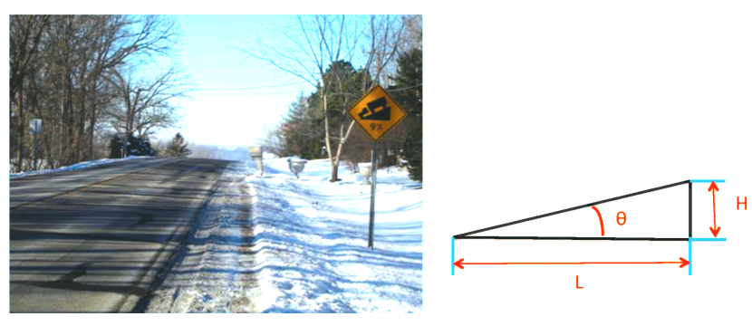
Figure 1: Highway grade sign and a right triangle to show slope.

The slope of a curve at a given point is defined as the slope of a tangent line at this point. Figure 2 shows three points: P, A and B. $T_{P}$ represents the tangent line at $P$ whose slope is defined as the slope of the curve at P. The tangent line’s slope is used to measure the curve’s steepness. Calculus studies (i) the slope $\tan\theta$ of a curve at various points, and (ii) the height increment $H$ from one point to another, say, A to B, as shown in Figure 2. Our geometric intuition indicates that height $H$ and slope $\tan\theta$ are related because $H$ increases rapidly if the slope is large for an upward trend. A core formula of calculus is to describe the relationship between these two quantities.

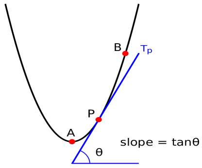
Figure 2: A curve, three points and a tangent line without coordinates.

Let us introduce the coordinates x and y and use a function $y=f(x)$ to describe the curve. We start with an example $f(x)=x^{2}$.

The tangent line of the curve at point $P(x_{0},y_{0})$ can be described by a point-slope equation

$$y-y_{0}=m(x-x_{0}),$$ (2)

where $y_{0}=x_{0}^{2}$, $m$ is the slope to be determined by the condition that the tangent line touches the curve at one point. In fact, “tangent” is a word derived from Latin and means “touch.”

The tangent line (2) and the curve

$$y=x^{2}$$ (3)

have a common point $P(x_{0},y_{0})$ (See Figure 3), where $x_{0}$ must be a double root, since the straight line is a tangent line.

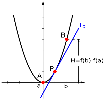
Figure 3: A curve, three points and a tangent line on xy-plane.

Substituting (3) to (2) to eliminate $y$, we have

$$x^{2}-x_{0}^{2}=m(x-x_{0}),$$ (4)

then

$$(x-x_{0})(x+x_{0})-m(x-x_{0})=0,$$ (5)

or

$$(x-x_{0})(x+x_{0}-m)=0.$$ (6)

The two solutions of this quadratic equation are

$$x_{1}-x_{0}=0$$ (7)

and

$$x_{2}+x_{0}-m=0$$ (8)

Since $P(x_{0},y_{0})$ is a tangent point, $x_{0}$ must be a repeated root, also called a double root. Hence, $x_{1}=x_{2}=x_{0}$. This yields

$$m=2x_{0}.$$ (9)

Thus, we claim that the slope of the curve $y=x^{2}$ at $x_{0}$ is $2x_{0}$, at $a$ is $2a$, at $3$ is $2\times 3=6$, and in general, at $x$ is $2x$. The slope measures the steepness of the curve $y=f(x)$, i.e., the rate of the curve’s height increase or decrease. The slope, or rate, varies from point to point. The slope is thus a derived quantity from the original function $y=f(x)$ and is called “derivative.” We have the following definition.

Definition 1. (Definitions of derivative as slope and DA pair). The slope $2x$ is called the derivative of $x^{2}$. Further, $x^{2}$ is called an antiderivative of $2x$. And ($2x$, $x^{2}$) is called a derivative-antiderivative (DA) pair.

For a general function $y=f(x)$, the slope of the curve $y=f(x)$ is called derivative and is denoted by $f^{\prime}(x)$ or $y^{\prime}$, and $f(x)$ is called antiderivative of $f^{\prime}(x)$. Thus, $(f^{\prime}(x),f(x))$ is a DA pair.

If $f(x)=C$ is a constant, then $y=C$ represents a horizontal line whose slope is $0$ for any $x$. Hence $(C)^{\prime}=0$, and $(0,C)$ is a DA pair.

If $f(x)$ is a linear function, then $y=\alpha+\beta x$ represents a straight line whose slope is $\beta$ for any $x$, hence $(\alpha+\beta x)^{\prime}=\beta$, i.e., $(\beta,\alpha+\beta x)$ is a DA pair.

Thus, the derivative’s geometric meaning is the slope of the curve $y=f(x)$: $f^{\prime}(x)$ is large at places where the curve $y=f(x)$ is steep. At a flat point, such as the maximum or minimum point of $f(x)$, the slope is zero since the tangent lines at these points are horizontal.

In addition to the geometric meaning, derivative has physical meaning, such as speed, and biological meaning, such as growth rate, as well as the meaning of the rate of change in almost any scientific field and anyone’s daily life. As an example, for a car driven at $v=60$ mph (miles per hour) for two hours, the total distance traveled is $s=v\times t=60\times 2=120$ mi. Here, $(v,vt)$ or $(v,s)$ is a DA pair for a general time $t$.

Free fall is another example. An object’s free fall has its distance of falling equal to $s=(1/2)gt^{2}$ and its falling speed is $v=gt$, where $g=32[ft/s^{2}]$ is the Earth’s gravitational acceleration. Galileo Galilei (1564-1642) discovered this time-square relationship for the distance. Since derivative $t^{2}$ with respect to $t$ is $2t$, we have $s^{\prime}=\frac{1}{2}g(2t)=gt$. Thus, $(gt,(1/2)gt^{2})$ or $(v,s)$ is a DA pair.

In general, the meaning of derivative is the rate of change of the function $f(x)$ with respect to the independent variable $x$, which can be either time or spatial location.

Let us now return to the derivative calculation. The above tangent line approach for finding the slope for $x^{2}$ can be applied to the function $y=x^{3}$. It is to solve the following simultaneous equations

$$y-y_{0}=m(x-x_{0}),$$ (10)

$$y=x^{3}.$$ (11)

Eliminating $y$, we have

$$x^{3}-x_{0}^{3}=m(x-x_{0}).$$ (12)

The factorization of this equation yields

$$(x-x_{0})(x^{2}+xx_{0}+x_{0}^{2}-m)=0.$$ (13)

This factorization implies $x_{1}-x_{0}=0$ and $x_{2}^{2}+x_{2}x_{0}+x_{0}^{2}-m=0$. The cubic equation has three solutions. Because $P(x_{0},y_{0})$ is the tangent point, $x_{0}$ is a repeated root of these two equations: $x_{1}=x_{2}=x_{0}$, which leads to

$$m=3x_{0}^{2}.$$ (14)

Hence, we claim that the derivative of $x^{3}$ is $3x^{2}$, and $x^{3}$ is an antiderivative of $3x^{2}$. Namely, ($3x^{2}$, $x^{3}$) forms a DA pair.

Following the tangent line approach, the above examples have demonstrated four DA pairs:

$$(0,C),\\ (1,x),\\ (2x,x^{2}),\\ (3x^{2},x^{3}).$$ (15)

The tangent line approach can be applied to any power function $x^{n}$, where $n$ is a positive integer. The DA pair for $x^{n}$ is

$$(nx^{n-1},x^{n}).$$ (16)

This formula actually holds for any real number $n$ with the exception of $n=0$. For example, $(x^{1/2})^{\prime}=(1/2)x^{-1/2}$. Proof of this claim is not easy, but fortunately the calculation of derivatives and antiderivatives can be easily done using computer programs. Many open source computer software packages are available to do this kind of calculation. For example, WolframAplha is one. At the website www.wolframalpha.com, you can enter a derivative command and a function, such as

derivative  x^(3/2)+4x^3

The computer will give you its derivative, plus other information, such as the graph of the derivative function (see Figure 4). You can also use WolframAlpha via a smart phone application.

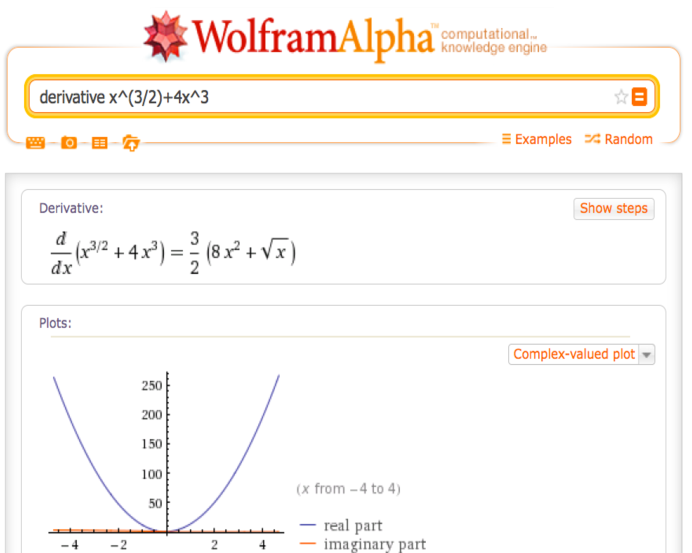
Figure 4: WalframAlpha derivative example.

To find an antiderivative, you can use a similar command

antiderivative  x^(3/2)+4x^3

Using this program, one can easily find DA pairs for commonly used functions. See the list below.

1. Exponential function: $(e^{x},e^{x})$.

2. Natural logarithmic function: $(\frac{1}{x},\ln x)$.

3. Sine function: $(\cos x,\sin x)$.

4. Cosine function: $(-\sin x,\cos x)$.

5. Tangent function: $(\sec^{2}x,\tan x)$.

3 Height increment and integrals

When we trace a curve, we care about not only the slope, but also the ups and downs of the curve, i.e., the increment or decrement of the curve from one point to another. When we drive over a mountain road, we also care about both steepness (i.e., slope) and elevation. Apparently, the slope and height increment are related. The slope has already been defined as derivative in the above section. In this section, the height increment is defined as integral, since the height increment or elevation increment is an integration process, or an accumulation process of point motion, measured by both speed and time.

For a function $y=f(x)$, its increment from $A(a,f(a))$ to $B(b,f(b))$ is $f(b)-f(a)$ as shown in Figure 3. Another notation for the increment is $f(b)-f(a)=f(x)|^{b}_{a}$. This height increment is used to describe the integral definition below.

Definition 2. (Definition of integral as height increment of a curve). The function’s increment $f(b)-f(a)$ from $A(a,f(a))$ to $B(b,f(b))$ is defined as the integral of the derivative function $f^{\prime}(x)$ in the interval $[a,b]$ and is denoted by $I[f^{\prime}(x),a,b]=f(b)-f(a)$. Here, $f^{\prime}(x)$ is called the integrand, and $[a,b]$ is called the integration interval.

Example 1. Given $f(x)=x$, $f^{\prime}(x)=1$, and $[a,b]=[0,2]$, we have

$$I[f^{\prime}(x),a,b]=I[1,0,2]=x|^{2}_{0}=2-0=2.$$ (17)

The area between $y=1$ and $y=0$ in the interval $[0,2]$ is also 2 (see Figure 5 for $f^{\prime}(x)=1,a=0$, and $b=1$).

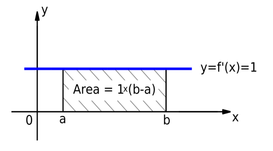
Figure 5: The area of a rectangle under a horizontal line.

Example 2. If we integrate speed $v(t)$, we will then get the distance $I[v(t),a,b]$ travelled from time $t=a$ to $t=b$. If $v(t)$ is a constant, say, $60$ mi/hour, and if $a=14:00$ and $b=16:00$, then the integral $I[60,14,16]=60t|_{14}^{16}=60\times(16-14)=120$ mi is the total distance traveled from 2pm to 4pm. Here $60t$ is an antiderivative of $60$. If we plot $v$ as a function of $t$, then $120$ is equal to the area of the rectangle bounded by $v=60,v=0,t=14$ and $t=16$ (See Figure 5 for $f^{\prime}(x)=60$, $a=14$, and $b=16$).

Example 3. Given $f(x)=(1/2)x^{2}$, $f^{\prime}(x)=x$, and $[a,b]=[0,1]$, we have

$$I[f^{\prime}(x),a,b]=I[x,0,1]=(1/2)x^{2}|_{0}^{1}=(1/2)(1^{2}-0^{2})=1/2.$$ (18)

The area under the integrand $y=x$ but above the $x$-axis in $[0,1]$ is $1/2$ (see Figure 6 for $a=0$ and $b=1$).

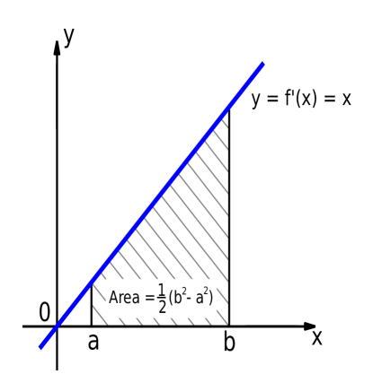
Figure 6: The area of a triangle under a straight line.

Example 4. In the free fall problem, the speed is a linear function of time, $v=gt$, and the integration $I[gt,0,x]=(1/2)gx^{2}$ is the distance traveled from time zero to time $x$. The region bounded by $v=gt,v=0,t=0$ and $t=x$ is a right triangle with base equal to $x$, height $gx$ and area $(1/2)\times x\times gx=(1/2)gx^{2}$. In this example, we have chosen to use $x$ as an arbitrary right bound for the region. This $x$ can can be any number, such as 1, 2, or 2.5.

In the above four examples, the area under a curve is equal to an integral. As a matter of fact, this inference of area equal to an integral is generally true. For an irregular region, we can simply use the integral $I[f^{\prime}(x),a,b]$ as the definition of the area of the region bounded by $y=f^{\prime}(x)$, $x$-axis, $x=a$ and $x=b$. The next section will justify this definition. As for the calculation of an integral, if one knows the relevant DA pair, the integral is a simple substitution $f(b)-f(a)$. Otherwise, one can use a computer to find the antiderivative, or to directly evaluate $I[f^{\prime}(x),a,b]$. Similar to derivative software, there are many free online computer programs and smart phone apps for calculating integrals. Figure 7 shows the WolframAlpha calculation of the integral $I[x^{4}+2x,0,1]$ using the command

integrate x^4+2x from 0 to 1

The result is 6/5. i.e., $I[x^{4}+2x,0,1]=6/5$.

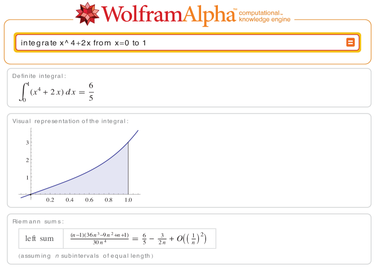
Figure 7: WalframAlpha integral example.

The definition of an integral states that the integral of a function in an interval is the increment of its antiderivative in the same interval. One can write

$$I[g(t),a,b]=G(b)-G(a)$$ (19)

where $G(t)$ is an antiderivative of $g(t)$. Another way to express the above is

$$I[G^{\prime}(u),a,b]=G(b)-G(a).$$ (20)

In the above two expressions, $t$ and $u$ are the integration variables, also called dummy variables. The integral values are independent of the choice of dummy variables. One can use any symbol to represent this variable. In practical applications, if the independent variable is time, such as when speed is a function of time, $t$ is often used as the independent variable.

Also according to the integral definition, the integral of $f^{\prime}(t)$ in the interval $[a,x]$ is

$$I[f^{\prime}(t),a,x]=f(x)-f(a).$$ (21)

Taking derivative of both sides of this equation with respect to $x$, we have

$$(I[f^{\prime}(t),a,x])^{\prime}_{x}=f^{\prime}(x)$$ (22)

since $(f(a))^{\prime}_{x}=0$ due to $f(a)$ being a constant with respect to $x$ and having a slope of zero. Here we have used a subscript $x$ to indicate that the independent variable is $x$ and the derivative is with respect to $x$.

Equation (22) is often called Part II of the Fundamental Theorem of Calculus (FTC), while the definition of an integral is actually often referred to as Part I of the FTC. Part II of the FTC is saying that an antiderivative can be explicitly expressed by an integral. Thus, the FTC makes a computable and close connection between slope and height increment, and enhances our intuitive sense that the height increment in an interval is closely related to the slope of our interested curve, i.e., our study function.

Example 5. $I[x,0,1]=(x^{2}/2)|^{1}_{0}=1^{2}/2-0^{2}/2=1/2$, because $(x,x^{2}/2)$ is a DA pair. The area between $y=x$ and $y=0$ over $[0,1]$ is 1/2 (=$I[x,0,1]$) (See Figure 6).

Example 6. $I[x^{2},0,1]=(x^{3}/3)|_{0}^{1}=1^{3}/3-0^{3}/3=1/3$, because $(x^{2},x^{3}/3)$ is a DA pair, or simply since $x^{2}$’s antiderivative is $x^{3}/3$. The area of the right triangle with a curved hypotenuse bound by $y=x^{2},y=0$ and $x=1$ is $1/3$ (=$I[x^{2},0,1]$) (See Figure 8). The WolframAlpha command for this calculation is integrate x3̂ from 0 to 1.

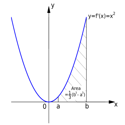
Figure 8: The area of a triangle of a curved hypotenuse when $a=0$.

4 Discussion and mathematical rigor of direct calculus

Two points are discussed here. First, is our definition of area by an integral reasonable and mathematically rigorous? Second, besides using computer programs to calculate the DA pairs of complicated functions, can one provide a systematic procedure of hand calculation?

First, how do we know that our definition of area using an integral is reasonable? According to the Oxford dictionary,“area” is defined as “the extent or measurement of a surface or piece of land.” The word “area” comes from the mid-16th century Latin, literally meaning a “vacant piece of level ground.” The units of an area are “square feet”,“square meters”, etc, meaning that the area of a region is equal to the number of equivalent squares, each side equal to a foot, a meter, or other units, that fit into the region. For the area between $y=f^{\prime}(x)$ and $y=0$ over $[a,b]$, the simplest measure is to use an equivalent rectangle of length $L=b-a$ and width $W$ (See Figure 9). That is, the excess area above $y=W$ (the vertically stripped region) is moved to fill the deficit area (the horizontally striped region). The corresponding description by a mathematical formula is below:

$$I[f^{\prime}(x),a,b]=L\times W=(b-a)\times W.$$ (23)

This can be true as long as we have

$$W=\frac{I[f^{\prime}(x),a,b]}{b-a}=\frac{f(b)-f(a)}{b-a}.$$ (24)

We call this $W$ the mean value of $f^{\prime}(x)$ over the interval $[a,b]$. Geometrically, $W=(f(b)-f(a))/(b-a)$ is the slope of the secant line that connects points $A$ and $B$ of Figure 10. If $y=f(x)$ is not a straight line, then there must be a point $m$ in $[a,b]$ whose slope is less than $(f(b)-f(a))/(b-a)$, and another point $M$ whose slope is larger than $(f(b)-f(a))/(b-a)$, i.e.,

$$f^{\prime}(m)\leq\frac{f(b-f(a)}{b-a}\leq f^{\prime}(M).$$ (25)

Between $f^{\prime}(m)$ and $f^{\prime}(M)$, $(f(b)-f(a))/(b-a)$ must meet the mid-ground slope $f^{\prime}(c)$ at a point $c$ in $[a,b]$, i.e.,

$$W=f^{\prime}(c)=\frac{f(b)-f(a)}{b-a}.$$ (26)

This is the mean value theorem (MVT) of calculus. It states that

Theorem 1. (MVT). There exists $c$ in $[a,b]$ such that $f^{\prime}(c)=\frac{f(b)-f(a)}{b-a}$ if $f^{\prime}(x)$ has a value for every $x$ in $[a,b]$.

Figure 9: An area interpretation of an integral.

Figure 10: Illustration of the mean value theorem: There is a tangent line parallel to the secant line connecting points $A$ and $B$.

Geometrically, MVT means that there is at least one point $c$ whose tangent line is parallel to the secant line $AB$. Of course, this holds if $y=f(x)$ is a straight line, in which case $c$ can be any point in $[a,b]$.

Rigorous mathematics for MVT would require one to prove the above statement “$(f(b)-f(a))/(b-a)$ must meet the mid-ground slope $f^{\prime}(c)$ at one point $c$ in $[a,b]$,” namely, it proves the existence of the point $c$. This is to prove the intermediate value theorem and is beyond the scope of this introductory lecture.

Therefore, the integral $I[f^{\prime}(t),a,x]=f(x)-f(a)$ is the increment of the antiderivative from $a$ to $x$, and is also the area for the region between the integrand derivative function and $y=0$ in the interval $[a,x]$, i.e., the region bounded by $y=f^{\prime}(t),y=0,t=a$ and $t=x$. The traditional definition of an integral is from the aspect of an area that is defined as a sum of many rectangles of increasing narrow widths, under the condition of each width approaching zero. For non-mathematics majors and general public, the condition of each width approaching zero, which is a concept of limit, adds complexity and confusion to the traditional definition of integral. In contrast, the geometric meaning of our direct integral is the height increment of the antiderivative, not the area underneath of the derivative. The area is only regarded as an additional geometric interpretation according to the intermediate value theorem. Under this interpretation of area, we have the following example.

Example 7. $I[\sqrt{1-x^{2}},0,1]$ is the area of a quarter unit round disc and is thus equal to $\pi/4$, since $y=\sqrt{1-x^{2}}$ represents a quarter circle in the first quadrant.

Calculating the slope using the factorization method works for polynomial functions, but the procedure is tedious. The procedure may not even work for transcendental functions like $y=\sin x$. The MVT provides another way to calculate the slope by using the slope of a secant line. In the above MVT, if $B$ moves very close to $A$, then the mean value $(f(b)-f(a))/(b-a)=f^{\prime}(c)$ in Theorem 1 is approaching the slope at $A$, since $c$ is approaching $a$, forced by $b$ approaching $a$. The formal writing is

$$\lim_{b\to a}\frac{f(b)-f(a)}{b-a}=f^{\prime}(a).$$ (27)

This can also be considered a definition of derivative and is called defining a derivative by a limit. This procedure is efficient to calculate the derivative by hand and to derive many traditional derivative formulas in the earlier years of calculus.

5 Descartes’ method of tangents and brief historical note

So, what is the origin of the direct calculus ideas described above? Numerous papers and books have discussed the historical development of calculus. Here we recount the development by a few major historical figures to sort out the origin of the main ideas of the calculus method outlined above. We cite only a few modern references and two works by Newton. Our focus is on (i) Descartes’ method of tangents that is the earliest systematic way of finding the slope of a curve without using a limit, and (ii) Wallis’ formulas of area, which were the earliest form of FTC. We do not intend to present a complete list of important works on the history of calculus.

In 1638, René Descartes (1596-1650) derived his method of tangents and included the method in his 1649 book, Geometry (see Cajori (1985), p.176). Descartes’ method of tangents is purely geometric, constructing a tangent circle at a given point of a curve with the circle’s center on the x-axis (Cajori (1985), pp. 176-177). Graphically, it is easier to draw a tangent circle than a tangent line using a compass and rulers. The tangent circle can be constructed using a radius line and moving the center on the x-axis so that the circle touches the curve at only one point. Then a tangent line can be drawn as the line perpendicular to the radial line of the circle at the tangent point.

Descartes’ method of tangents also has an analytic description. The tangent circle is determined by the given point $P(x_{0},y_{0})$ on the curve and the moving center on the x-axis $(a,0)$. The circle’s equation is

$$(x-b)^{2}+(y-0)^{2}=(x_{0}-a)^{2}+(y_{0}-0)^{2}.$$ (28)

The tangent condition requires that this equation and the curve’s equation $y=f(x)$ have a double root at $P(x_{0},y_{0})$. This can determine $a$ and hence the tangent circle. The radial line is determined by $P(x_{0},y_{0})$ and $(a,0)$ and has its slope $m_{R}=y_{0}/(x_{0}-a)$. The tangent line of the circle at point $P(x_{0},y_{0})$ is the tangent line of the curve at the same point. The slope of the tangent line is calculated as $m_{T}=-1/m_{R}=(a-x_{0})/y_{0}$. In the above procedure, limit is not used.

Example 8. Use Descartes’ method of tangents to find the slope of $y=\sqrt{x}$ at $(1,1)$.

Substituting $y=\sqrt{x}$ into eq. (28), we obtain

$$(x-a)^{2}+x=(1-a)^{2}+1.$$ (29)

This can be simplified to

$$x^{2}+(1-2a)x+2(a-1)=0.$$ (30)

Knowing that $x=1$ is a solution of this equation helps factorize the left-hand side

$$(x-1)(x+2-2a)=0.$$ (31)

The double root condition for a tangent line requires $x_{1}=x_{2}=1$. This leads to

$$x_{2}+2-2a=1+2-2a=0.$$ (32)

Hence, $a=3/2.$ The slope of the radial line is $m_{R}=1/(1-3/2)=-2$. The slope of the tangent line is thus $m_{T}=1/2$.

Although Descartes’ method of tangents is complicated in calculation, its concept is simple, clear and unambiguous, and its geometric procedure is sound. It does not involve small increments of an independent variable (developed by Fermat also in the 1630s), and hence it does not involve limits or infinitesimals. According to the point-slope equation of a tangent line presented earlier, the complexity of Descartes’ method of tangents is unnecessary to calculate a slope. However, the point-slope form of a line was not known during Descartes’ lifetime. According to Range [6], the point-slope form of a line was first introduced explicitly by Gaspard Monge (1746-1818) in a paper published in 1784. Thus, Monge’s point-slope method of tangent appeared more than 100 years after Descartes’ method of tangents.

Pierre de Fermat (1601-1665)’s method of tangents is similar to the modern method of differential quotient and uses a small increment (i.e., infinitesimal), which is ultimately set to be zero when the infinitesimal is forced to disappear from the denominator (Ginsburg et al., 1998). Thus, Fermat’s method of tangents is more efficient for calculation from the point of view of limit, while Descartes’ method of tangents is geometrically more direct and easier to plot by hand, and Monge’s method of tangents is geometrically more direct. Fermat also used a sequence of rectangular strips to calculate the area under a parabola. His strips have variable width, which enabled him to use the sum of geometric series. This method of calculating an area can be traced back to Archimedes.

Archimedes (287-212 BC) ’s method of exhaustion enabled him to find the area under a parabola. He used infinitely many triangles inscribed inside the parabola and also utilized the sum of geometric series.

Bonaventura Cavalieri (1589-1647) used rectangular strips of equal width to calculate the area under a straight line (i.e., a triangle) and under a parabola.

Around 1655-1656, John Wallis (1616-1703) derived algebraic formulas that represent the areas under the curve of simple functions, such as $y=kt$ and $y=kt^{2}$, from $0$ to $x$ (Ginsburg et al., 1998). Considering the existing work on tangents (i.e., slopes or derivatives) at that time, and considering the DA pair concept here, we thus may conclude that Wallis had already explicitly demonstrated, before Newton, the relationship between slope and area using examples, i.e., FTC.

Isaac Newton (1642-1727) attended Trinity College, Cambridge in 1660 and quickly made himself a master of Descartes’ Geometry. He learned much mathematics from his teacher and friend Isaac Barrow (1630-1677), who knew the method of tangents by both Descartes and Fermat and also knew how to calculate areas under some simple functions. Barrow revealed that differentiation and integration were inverse operations, i.e., FTC (Cajori, 1985). Newton summarized the past work on tangents and area calculation, introduced many applications of the two operations, and made the tangent and area methods a systematic set of mathematics theory. Newton’s method of tangents followed that of Fermat and had a small increment that eventually approaches zero. Namely, he used a sequence of secant lines to approach a tangent line as is done in modern calculus’ definition of derivative. Although the “method of limits” is frequently attributed to Newton (see his book (Newton, 1729) entitled “The Mathematical Principles of Natural Philosophy” (p45)), he was not as adamant as Leibniz about letting an infinitesimal be zero at the end of a calculation. Newton was dissatisfied with the omitted small errors. He wrote that “in mathematics the minutest errors are not to be neglected” (see Cajori (1985), p198).

Newton’s method of fluxions intended to solve two fundamental mechanics problems that are equivalent to the two geometric problems of slope and height increment of a curve pointed out earlier in in this paper:
“(i). The length of the space described being continually (i.e., at all times) given; to find the velocity of the motion at any time proposed.
(ii). The velocity of motion being continuously given; to find the length of the space described at any time proposed” (see Cajori (1985), p.193, and Newton (1736), p.19).

The solution to these two problems also led to FTC, as geometrically interpreted in previous sections. The above statement of the two problems is directly cited from Newton’s book “The Method of Fluxions ”(Newton (1736), p.19), which was translated to English from Latin and published by John Colson.

Gottfried Wilhelm Leibniz (1646-1716) produced a profound work similar to Newton’s that summarized the method of tangents and the method of area using a systematic approach. His approach has been passed on to today’s classrooms, including his notations of derivative and integration.

Our description of calculus method has demonstrated that if we avoid calculating the area underneath a curve and define an integral by the height increment, we can readily extend Descartes’ method of tangents to establish the theory of differentiation and integration by considering the slope (i.e., grade), DA pair, and height increment. The no-limit approach to calculus outlined in this paper is attributable to Descartes’ original ideas, and is different from the those of Fermat, Newton and Leibniz. The FTC is attributable to Wallis’ original ideas. Ginsburg et al. (1998) concluded that the query whether Leibniz plagiarized Newton’s work on calculus is not really a valid question since the calculus ideas had already been developed by others before the calculus works of either Newton or Leibniz. Both just summarized the work of earlier mathematicians and developed differentiation and integration into a systematic branch of mathematics by using the methods of infinitesimals and limits. After their work, calculus became a very useful tool in engineering, natural sciences, and numerous other fields.

In addition to the aforementioned mathematicians, there are many others who contributed to the development of calculus, including Gregory of St. Vincent (1584-1667) from Spain, Gilles Persone de Roberval (1602-1675), Blaise Pascal (1623-1662), Christiaan Huygens (1629-1695), and Leonhard Euler (1707-1783). Augustin-Louis Cauchy (1789-1857) has been credited with the rigorous development of calculus from the definition of limits. Karl Weierstrass (1815-1897) corrected Cauchy’s mistakes and introduced the delta-epsilon language we use today in mathematical analysis.

6 Conclusions

We have introduced the concepts of derivatives and integrals without using limits. Geometrically, derivatives were introduced directly from the slope of a tangent line. Algebraically, derivatives and antiderivatives were introduced simultaneously as a DA pair. Then the integral was introduced as the height increment of the antiderivative function. This increment was geometrically interpreted as the area of the region bounded by the integrand function, the horizontal axis and the integration interval. A justification of this interpretation was given to demonstrate that this definition of area was reasonable and mathematically rigorous up to the proof of IVT which, like the Euclidean axioms, is intuitively true to most people in general public. At the end, we pointed out that limit was an efficient approach to calculate derivatives by hand and could help derive derivative formulas for complicated functions besides polynomials. We thus regard that the limit approach to calculus is an excellent computing method for finding derivatives by hand. In the pre-computer era, this limit approach was obviously critical in calculating derivatives of a variety of functions. In our current computer era, the limit approach to calculus is less essential and may be unnecessary for non-mathematical majors or general public at the introductory stage.

Although the ideas of direct calculus described in this paper come from practical applications, we have maintained the self-contained mathematical rigor and logic. Pure mathematical analysis regarding the structure of real line and the sequence approach to a compact set are not topics for this introduction. These analysis approaches mainly due to Cauchy and Weierstrass have certainly enriched calculus as begun by Archimedes, Descartes, Fermat, Wallis, Newton, Leibniz and others. However, our paper has shown that it is possible to introduce the basic concepts and calculation methods of calculus directly, without using limits.

One can also regard calculus as an extension of the trigonometry of a regular right triangle to the trigonometry of a curved-hypotenuse right triangle. For a regular right triangle, the slope (i.e., derivative = tangent of the angle) of the hypotenuse is derivative, and the vertical increment (i.e., an integral) is equal to the opposite side, which is the integral of the derivative (see Figure 11). It is obvious that the vertical increment and the slope are related and have the following relationships:

$$\tan\theta=\frac{BC}{AC}\qquad\mbox{(derivative)}$$ (33)

and

$$BC=\tan\theta\times AC\qquad\mbox{(integral)}.$$ (34)

These two formulas are the FTC for the regular right triangle. The extension is from this straight line hypotenuse to the curved hypotenuse, such as a parabola or an exponential function. For the curved hypotenuse, the slope varies at different points and the total height increment is an integral. That is,

$$m=f^{\prime}(x)\qquad\mbox{(derivative)}$$ (35)

and

$$BC=I[f^{\prime}(x),a,b]\qquad\mbox{(integral)}.$$ (36)

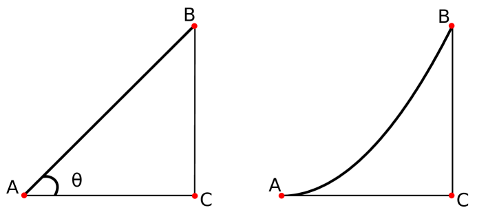
Figure 11: Calculus explained by triangles with straight and curved hypotenuses

Acknowledgments.   Julien Pierret, Jazlynn Ngo, and Kimberly Leung assisted with plotting the figures in this paper. The discussion with Chris Rasmussen and Dov Zakis was helpful in the paper’s development. The work was partially supported by the US National Science Foundation. During his many visits to China, the lead author, Samuel S.P. Shen, exchanged ideas and worked together with the second author, Qun Lin. The original ideas and technical details of this paper are credited to the lead author.

References

1. F. Cajori, A History of Mathematics (pp. 162-198), 4th ed., Chelsea Publishing Co., New York, 534pp, 1985.

2. J.L. Coolidge, The story of tangents. American Math. Monthly 58 (1951) 449-462.

3. D. Ginsburg, B. Groose, J. Taylor, and B. Vernescu, The History of the Calculus and the Development of Computer Algebra Systems, Worcester Polytechnic Institute Junior-Year Project, www.math.wpi.edu/IQP/BVCalcHist/calctoc.html, 1998

4. Q. Lin, Calculus for High School Students: from a Perspective of Height Increment of a Curve, People’s Education Press, Beijing, 2010.

5. Q. Lin, Fastfood Calculus, Science Press, Beijing, 2009.

6. I. Newton, The Method of Fluxions and Infinite Series with Application to the Geometry of Curve-Lines, Translated from Latin to English by J. Colson, Printed for Henry Woodfall, London, 339pp, 1736. [http://books.google.com]

   http://books.google.com/books?id=WyQOAAAAQAAJ&printsec=frontcover&source=
   gbs_ge_summary_r&cad=0#v=onepage&q&f=false
   

7. I. Newton, The Mathematical Principles of Natural Philosophy, Translated from Latin to English by A. Motte, Printed for Benjamin Motte, London, 320pp, 1729. [http://books.google.com]

   http://books.google.com/books?id=Tm0FAAAAQAAJ&printsec=frontcover&source=
   gbs_ge_summary_r&cad=0#v=onepage&q&f=true
   

8. R.M. Range, Where are limits needed in calculus? Amer Math Monthly 118 (2011) 404-417.

9. J. Susuki, The lost calculus (1637-1670): Tangency and optimization without limits. Mathematics Mag. 78 (2005) 339-353.