Magnetic states of the five-orbital Hubbard model for
one-dimensional iron-based superconductors

Abstract

The magnetic phase diagrams of models for quasi one-dimensional compounds belonging to the iron-based superconductors family are presented. The five-orbital Hubbard model and the real-space Hartree-Fock approximation are employed, supplemented by density functional theory to obtain the hopping amplitudes. Phase diagrams are constructed varying the Hubbard $U$ and Hund $J$ couplings and at zero temperature. The study is carried out at electronic density (electrons per iron) $n=5.0$, which is of relevance for the already known material TlFeSe₂, and also at $n=6.0$, where representative compounds still need to be synthesized. At $n=5.0$ there is a clear dominance of staggered spin order along the chain direction. At $n=6.0$ and the realistic Hund coupling $J/U=0.25$, the phase diagram is far richer including a variety of “block” states involving ferromagnetic clusters that are antiferromagnetically coupled, in qualitative agreement with recent Density Matrix Renormalization Group calculations for the three-orbital Hubbard model in a different context. These block states arise from the competition between ferromagnetic order (induced by double exchange, and prevailing at large $J/U$) and antiferromagnetic order (dominating at small $J/U$). The density of states and orbital compositions of the many phases are also provided.

I Introduction

The theoretical study of high critical temperature iron-based superconductorsjohnston2010 was initially centered on the concept of Fermi surface (FS) nesting, within a framework that assumes a weak on-site Hubbard $U$ coupling strength. However, a variety of recent experiments have indicated that there are serious deviations from this simplistic scenario.dai2012 For example, robust local moments have been found at room temperaturelocal that are incompatible with a weak coupling perspective where both the local moments and long-range magnetic order should develop simultaneously upon cooling. The existence of nematic statesdavis and orbital-independent superconducting gapsshimojima are other experimental observations that cannot be rationalized merely by FS nesting. At present, from the results of several experiments and calculations there is a convergence to the notion that these materials are in an “intermediate” coupling regime with regards to the strength of the Hubbard $U$ interaction.dai2012 ; basov ; rong2009 ; luo-neutrons ; DFT+DMFT ; Kotliar This coupling regime certainly represents a challenge to theorists because standard many-body techniques are not sufficiently developed to study with accuracy the difficult intermediate $U$ regime. In addition, the nature of the problem requires using complex multiorbital Hubbard models that are considerably more difficult to study than the simpler one-orbital models used for cuprates.

Adding to the complexity that emerges from these recent investigations is the discovery of insulating states in alkali metal iron selenides, with a chemical composition very close to those of superconducting samples.dagotto2013 In particular, a novel magnetic state of the iron superconductors was reported for the intercalated iron selenide K_0.8Fe_1.6Se₂, with iron vacancies in a $\sqrt{5}\times\sqrt{5}$ arrangement. Neutron scattering studiesbao of this (insulating) compound revealed an unusual spin arrangement involving 2$\times$2 iron blocks with their four spins ferromagnetically ordered, supplemented by an in-plane antiferromagnetic coupling of these 2$\times$2 magnetic blocks. K_0.8Fe_1.6Se₂ also has a large ordering temperature and large individual magnetic moments $\sim$3.3 $\mu_{B}$/Fe. Note that phase separation tendencies have also been reported in this type of materials,ricci and for this reason the relation between the exotic magnetic order involving ferromagnetic blocks described above and superconductivity is also a matter of intense discussion.

These developments suggest that new insights into iron pnictides and chalcogenides could be developed if the iron spins are arranged differently than in the nearly square geometry of the FeSe layers. For this reason considerable interest was generated by recent studiescaron1 ; petrovic ; caron2 ; nambu ; Sefat of BaFe₂Se₃ (123) that contains substructures with the geometry of two-leg ladders, similarly as those widely discussed before in the context of Cu-based superconductors.ladders-original ; dagotto-rice ; dagotto-ladder Neutron diffraction studies of the 123-ladder at low temperature caron1 ; nambu reported a magnetic order involving blocks of four iron atoms with their moments aligned, coupled antiferromagnetically along the “leg” ladder direction. This “Block-AFM” state is similar to that discussed before for K_0.8Fe_1.6Se₂, with the iron vacancies. When the 123-ladder material is hole doped with K, the magnetic state evolves from the Block-AFM state to a spin state (called CX) for the case of KFe₂Se₃ with ferromagnetically align spins along the rungs, coupled antiferromagnetically along the legs of the ladders.caron2 Adding to the importance of these novel ladder materials, a single layer of alkali-doped FeSe with the geometry of weakly coupled two-leg ladders was recently reported to be superconducting.SCladder These Fe-based ladders provide a simple playground where superconductivity and magnetism can be explored, in a geometry that simplifies the theoretical studies due to its quasi one-dimensionality.

In recent real-space Hartree-Fock (HF) calculations of ladder models,luo2013-ladders the 2$\times$2 Block-AFM state was indeed found to be stable in a robust region of parameter space, after a random initial magnetic configuration was used as the start of the iterative process to avoid biasing the results. The other recently observedcaron2 CX-state was also found in the theoretical phase diagrams. Several other competing states, that could be stabilized in related compounds via chemical doping or high pressure, were also identified.luo2013-ladders The variety of possible magnetic states is remarkable, revealing an unexpected level of complexity in these systems. A technical aspect important for our purposes is that the study in Ref. luo2013-ladders, showed that the use of the HF technique, which is a crude approximation particularly in a low-dimensional geometry, did capture the essence of the magnetic order in ladders at least when compared with Density Matrix Renormalization Group calculations. This previous agreement allow us to be confident that a HF study in one dimension, as presented below, may still capture the dominant correlations at short distances in the phase diagrams.

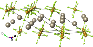
Figure 1: Crystal structure of the one-dimensional compound TlFeSe₂. The spheres with small, medium, and large size represent Se, Fe, and Tl atoms, respectively. The primitive unit cell and its lattice vectors are also shown.

In addition to the BaFe₂Se₃ compound already mentioned, there is another group of Fe-selenide materials that also display quasi one-dimensional characteristics but in this case simply involving chains as opposed to ladders. A typical representative is TlFeSe₂. Its crystal structure is in Fig. 1, and it contains dominant substructures in the form of weakly coupled chains.veliyev ; seidov Iron is in a state Fe³⁺, which corresponds to $n=5$ for the electronic population of the $3d$ Fe orbitals ($n$ is the average number of electrons in the $3d$ shell of the iron atoms). TlFeSe₂ is believed to be antiferromagnetic, based on magnetic susceptibility and transport measurements, with a characteristic temperature $\sim 290$ K where short-range order along the chains develops,veliyev followed upon cooling by the stabilization of three-dimensional long-range order at a lower temperature $\sim 14$ K. As a consequence, over a wide temperature range the material behaves as nearly-independent quasi-one dimensional chains. There are other compounds with similar structures,veliyev ; seidov ; K-1D such as TlFeS₂ and KFeSe₂. In particular, TlFeS₂ has been studied with neutron diffraction and it is also believed to be antiferromagnetic at low temperatures.weiz In spite of all this progress, the microscopic details of the spin order arrangements are unknown.

It is interesting to recall that in the context of the Cu-based superconductors the study of materials that contain dominant one-dimensional chain substructures, such as SrCuO₂ srcuo2 and Sr₂CuO₃,sr2cuo3 as well as the already mentioned two-leg ladders,ladders-original ; dagotto-rice ; dagotto-ladder led to considerable advances in the understanding of cuprates. For all these reasons, in the present effort the theoretical study of the magnetic states of models for one-dimensional iron-based superconductors will be initiated. Our aim is to present a HF comprehensive study of multiorbital Hubbard models in one dimension to predict qualitatively the dominant magnetic states in this context, thus guiding future neutron scattering experiments. The previously discussed success in the use of the HF approximation when applied to ladders give us confidence that at least qualitatively this crude approximation may still reveal the dominant magnetic tendencies in one-dimensional systems. Of course, it is important to realize that long-range order in the HF sense may in practice only correspond to dominant power-law behavior in a particular ordering channel for the one-dimensional systems of interest here, or merely short-range order tendencies.

The electronic density $n=5$ of relevance for TlFeSe₂ will be studied here, but other electronic densities, such as $n=6$ which is of relevance in two-dimensional pnictides, will also be analyzed. This extension in the range of $n$ is in anticipation of the possible synthesis of novel one-dimensional materials with other values of $n$ in the future. In general terms, our overarching goal is to motivate further experimental and theoretical efforts in the study of one-dimensional iron-based materials since their theoretical analysis is simpler than in two dimensions and considerable insight on these exotic compounds can be gained by their detailed study and subsequent comparison with experiments.

The organization of the manuscript and our main results are the following. In Sec. II, details of the density functional theory calculation are described, together with the five-orbital Hubbard model and the many-body technique employed. Section III contains the phase diagrams at both densities $n=5$ and $6$, in one and in anisotropic two dimensions. Section IV contains the density of states and orbital composition. Finally, the conclusions are provided in Sec. V. The details of the hopping amplitudes are provided in the Appendix.

II Model and Technique

The theoretical work presented in this section consists of two parts. First, using $ab$-$initio$ techniques the band structure of TlFeSe₂ was calculated, and tight-binding hopping amplitudes were deduced. Second, using the band structure information, Hubbard models involving the five $3d$ orbitals of Fe were constructed and studied with HF approximations. The detail is the following:

II.1 Band structure calculation

The electron Fe-Fe hopping amplitudes corresponding to the five Fe $3d$ orbitals in TlFeSe₂ were calculated using two independent density functional theory (DFT) approximations. In the first one, the all-electron linearized augmented plane wave method, as implemented in WIEN2k w2k with the Perdew-Burke-Ernzerhof approximation for the exchange-correlation functional,PBE was employed to obtain the electronic structure of TlFeSe₂, which was subsequently projected onto a Wannier functions basis.Aichhorn09 The second calculation has been carried out in the frame of the local spin density approximation with the Perdew and Zunger (PZ) exchange-correlation functional,PZ using the plane wave pseudopotential method as implemented in the PWSCF code of the Quantum ESPRESSO (QE) distribution.QE The ultrasoft pseudo-potentialUSPSPOT optimized in the RRKJ schemeRRKJ was used (Se.pz-n-rrkjus.UPF, Fe.pz-spn-rrkjus.UPF from the QE pseudopotentials database were employed, while the Pb.pz-dn-rrkjus.UPF pseudopotential was used as a prototype for the Tl pseudopotential). Furthermore, the result was used to calculate Maximally Localized Wannier functions MLWF as it is implemented in the Wannier90 distribution.W90 Since the difference between hopping amplitudes obtained by these two methods does not exceed a few percent, for simplicity below only the WIEN2k results will be used.

The DFT calculations presented here are based on the crystal structure refined by Klepp and Boller.Klepp79 TlFeSe₂ belongs to the $C2/m$ space group with a monoclinic centered unit cell (Fig. 1). The edge-sharing FeSe₄-tetrahedra form layers of parallel chains with slightly alternating nearest-neighbor Fe-Fe bond distances in the $ac$-plane of the primitive unit cell, separated by Tl atoms; each primitive unit cell contains two formula units.

According to the DFT calculations, the Fe and Se states are strongly hybridized, with the Fe $3d$ character prevailing between -1.8 and 1.5 eV (Fermi level is at 0 eV). This energy range was used to construct the projected Fe $3d$ Wannier functions and calculate the corresponding hopping integrals. The final tight-binding (TB) model, used in our model calculations, includes all hoppings between the Fe pairs in the plane of Fe chains within the separation range of 8.24 Å. After the model is constructed, different electronic densities will simply be reached by changing a chemical potential.

The DFT-calculated values of some of the hopping amplitudes are in the Appendix. As expected, the nearest-neighbor hoppings along the Fe-chains are dominant, with the largest absolute value being approximately 0.43 eV. However, in order to reproduce accurately the fine details of the band structure it is necessary to consider quite a number of longer-ranged hoppings in other directions as well. Thus, a judicious truncation of the hopping range (details presented below) must be carried out to render practical the HF approximation described below.

II.2 Hubbard model setup and many-body technique

A multi-orbital Hubbard model will be employed in this study, based exclusively on the Fe $3d$ electrons. Our emphasis will be on the magnetic states obtained by varying the coupling parameters. This Hubbard model includes all five Fe $3d$ orbitals $\{d_{z^{2}},d_{x^{2}-y^{2}},d_{xy},d_{xz},d_{yz}\}$, which are widely believed to be the most relevant orbitals at the Fermi surface for the iron-based superconductors, in agreement also with the band structure calculations of the previous subsection.

In real space, this multi-orbital Hubbard model includes a tight-binding term defined as:

$$H_{\rm TB}=\sum_{<\mathbf{i,j}>}\sum_{\alpha,\beta,\sigma}t^{\alpha\beta}_{ij}(c^{\dagger}_{\mathbf{i},\alpha,\sigma}c_{\mathbf{j},\beta,\sigma}+h.c.),$$ (1)

where $c^{\dagger}_{\mathbf{i},\alpha,\sigma}$ creates an electron with spin $\sigma$ in the orbital $\alpha$ at site $\mathbf{i}$, and $t^{\alpha\beta}_{ij}$ refers to the tunneling amplitude of electron hoppings from orbital $\alpha$ at site $\mathbf{i}$ to orbital $\beta$ at site $\mathbf{j}$. The Coulombic interacting portion of the multi-orbital Hubbard Hamiltonian is given by:

$$\begin{split}H_{\rm int}&=U\sum_{{\bf i},\alpha}n_{{\bf i},\alpha,\uparrow}n_{{\bf i},\alpha,\downarrow}+(U^{\prime}-J/2)\sum_{{\bf i},\alpha<\beta}n_{{\bf i},\alpha}n_{{\bf i},\beta}\\ &\quad-2J\sum_{{\bf i},\alpha<\beta}{\bf S}_{\bf{i},\alpha}\cdot{\bf S}_{\bf{i},\beta}\\ &\quad+J\sum_{{\bf i},\alpha<\beta}(d^{\dagger}_{{\bf i},\alpha,\uparrow}d^{\dagger}_{{\bf i},\alpha,\downarrow}d^{\phantom{\dagger}}_{{\bf i},\beta,\downarrow}d^{\phantom{\dagger}}_{{\bf i},\beta,\uparrow}+h.c.),\end{split}$$ (2)

where $\alpha,\beta=1,2,3,4,5$ denote the Fe $3d$ orbitals, ${\bf S}_{{\bf i},\alpha}$ ($n_{{\bf i},\alpha}$) is the spin (electronic density) of orbital $\alpha$ at site ${\bf i}$ (this index labels sites of the square lattice defined by the irons), and the standard relation $U^{\prime}=U-2J$ between the Kanamori parameters has been used. The first two terms give the energy cost of having two electrons located in the same orbital or in different orbitals, both at the same site, respectively. The second line contains the Hund’s rule coupling that favors the ferromagnetic (FM) alignment of the spins in different orbitals at the same lattice site. The “pair-hopping” term is in the third line and its coupling is equal to $J$ by symmetry.

In this effort, the Hartree-Fock approximation will be applied to the Coulombic interaction, restricted to act only “on site”, to investigate the ground state properties. This HF approximation results in a HF Hamiltonian containing several unknown HF expectation values (due to the many combinations of orbitals that can be made). All these expectation values need to be optimized by a self-consistent iterative numerical process. The expectation values are assumed independent from site to site in the numerical procedure, allowing the system to select spontaneously the state that minimizes the HF energy, thus reducing the bias into the calculations. To start the self-consistent iteration process, first all the HF expectation values are set to some randomly chosen numbers, defining a random initial state. These random-start process tends to be time consuming and at the end of the iterations states are obtained that typically display close, but not perfect, regularity. By hand, these imperfections are removed and then those regular states are used again as initial states in the HF iterative process where they are further optimized.

At the end of this tedious procedure, the ground states are selected by comparing the final ground energies after convergence. As discussed before, the tight-binding hopping amplitudes are obtained from the DFT calculation. However, for comparison purposes results using the hoppings from Ref. Graser08, , which were deduced in a quite different context, will be used as well to judge how robust our HF results phase diagrams are. Our conclusions are that the essence of the phase diagrams do not depend much on the details of the hoppings.

The HF calculations reported here are carried out using three different lattices: (1) Our most important results are obtained on $32\times 1$ clusters, namely on one-dimensional single chains. Here, only the hopping amplitudes along the Fe-chain direction (See Fig. 1 in the Appendix) are employed, including $t^{11}_{[0,0]}$, $t^{12}_{[0,0]}$, $t^{12}_{[-1,1]}$, $t^{11}_{[-1,1]}$, $t^{11}_{[1,-1]}$, $t^{12}_{[1,-1]}$ and $t^{12}_{[-2,2]}$. The ratio of hopping amplitudes at maximum and minimum distances is $t^{12}_{[0,0]}/t^{12}_{[-2,2]}\approx 12$. (2) Also $16\times 1$ one-dimensional single chains were used but employing the hopping amplitudes from Ref. Graser08, . The ratio of hopping amplitudes at maximum and minimum distances is about $12$ in this case as well. (3) To develop at least a qualitative idea of the magnetic coupling between the one-dimensional dominant structures, $8\times 8$ two-dimensional square lattices were also studied. All the hopping amplitudes presented in the Appendix were employed in this case.

Periodic boundary conditions (PBC) are used here for all the calculations. In the self-consistent iterative process, the criteria of convergence is set so that the changes of the HF expectation values are less than $10^{-4}$. Under this criteria, the typical number of iterations can be as large as $10,000$ for the two-dimensional calculations and as large as $5,000$ for the one-dimensional calculations, particularly for the case of random starting configurations.

III Results

III.1 Electronic density $n$=5 with (truncated to 1D) TlFeSe₂ hoppings

Let us start our description of the main results with the case of electronic density $n=5$, corresponding to TlFeSe₂, and using first a one-dimensional system containing 32 sites, and employing the real-space HF technique described in the previous section. Increasing the Hubbard coupling $U$ to move beyond the paramagnetic regime and for all the Hund couplings $J$ analyzed here, there is only one magnetic state in the entire phase diagram, namely the staggered $\uparrow\downarrow\uparrow\downarrow$ state denoted as AF1 in Fig. 2. This type of magnetic order is quite natural in an electronic density regime with one electron per orbital at every site.

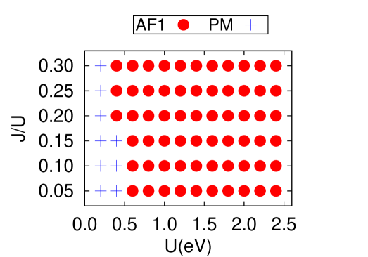
Figure 2: Phase diagram obtained using a $32\times 1$ one-dimensional lattice, employing the real-space HF technique at a fixed electronic density $n=5.0$. AF1 simply denotes a staggered AFM state, namely a pattern of spins $\uparrow\downarrow\uparrow\downarrow$ [see Fig. 3(b)]. The “Paramagnetic” (PM) state was defined with the following convention: the order parameter $m$ is smaller than a cutoff value chosen as $5\%$ of the saturated value for the same state at larger $U$ couplings. The hopping amplitudes used for this chain are in the hopping matrices along the Fe-chain direction shown in the Appendix section, including $t^{11}_{[0,0]}$, $t^{12}_{[0,0]}$, $t^{12}_{[-1,1]}$, $t^{11}_{[-1,1]}$, $t^{11}_{[1,-1]}$, $t^{12}_{[1,-1]}$ and $t^{12}_{[-2,2]}$. The bandwidth at $U=J=0$ is $W=2.36$ eV.

It should be remarked that there are two-dimensional analogs of the case described here that also have the same staggered magnetic order. To be more precise, in recent efforts a new avenue of research in iron-based superconductors has been expanding. It consists of replacing entirely Fe by Mn or other $3d$ transition elements. The average electronic population of the $3d$ orbitals of Mn is $n=5$, different from the $n=6$ of Fe, but the crystal structures are similar as in layered iron pnictides. As example, in the case of the 100% replacement of Fe by Mn, the compound BaMn₂As₂ was found to develop a G-type AFM state with staggered spin order, a Néel temperature of 625 K, and a magnetic moment of 3.88$\mu_{B}$/Mn at low temperatures.BMA The G-type AFM order appears to be very robust, as recent investigations of Ba_1-xK_xMn₂As₂ have shown.persistence Again, this state emerges naturally from the population $n=5$ at each Mn atom, namely one electron per $3d$ orbital. For the same reason, it is natural that in our one-dimensional case at $n=5$ a similar dominance of staggered spin order is found.

III.2 Magnetic phase diagram for chain systems at electronic density $n$=6

The phase diagrams become far richer when the electronic density is changed away from $n=5$. Figure 3 contains results that are expected to apply to materials with electronic density $n=6.0$ that still have not been synthesized to our knowledge. As in the previously described results, in this subsection the case of an isolated chain is investigated since the hoppings perpendicular to the chains are first neglected. In TlFeSe₂ there is a robust range of temperatures where the physics is expected to be dominated by the one-dimensional structures, and it is in this regime that the present results are the most important if such a broad temperature window for one dimensionality also exists in the yet-to-be-made $n=6$ materials. In the absence of concrete information about possible $n=6$ chain compounds, here the same hoppings as for the $n=5$ case of TlFeSe₂ case are used.

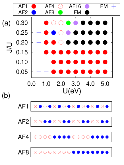
Figure 3: (a) Phase diagram obtained using a $32\times 1$ one-dimensional lattice, employing real-space HF techniques at a fixed electronic density $n=6.0$. The “Paramagnetic” (PM) state was defined with the following convention: the order parameter $m$ is smaller than a cutoff value chosen as $5\%$ of the saturated value for the same state at larger $U$ couplings. The hopping amplitudes used for this chain are the hopping matrices along the Fe-chain direction (see Appendix section), including $t^{11}_{[0,0]}$, $t^{12}_{[0,0]}$, $t^{12}_{[-1,1]}$, $t^{11}_{[-1,1]}$, $t^{11}_{[1,-1]}$, $t^{12}_{[1,-1]}$ and $t^{12}_{[-2,2]}$. The bandwidth at $U=J=0$ is $W=2.36$ eV. (b) Sketches of the states found in the phase diagram shown in (a), and their labeling convention.

Figure 3 (a) contains the phase diagram varying the Hubbard $U$ and Hund $J$ couplings at electronic density $n=6$. The complexity of the phase diagram, far richer than for the case $n=5$, is clear. The detail of the magnetic patterns in the many competing states is in Fig. 3 (b). At small $U$, Fig. 3 (a) has a paramagnetic state as expected. Increasing $U$, the spin staggered AF1 state is stabilized. This occurs even at large values of $U$ as long as $J/U$ remains at 0.15 or below. However, in the more realistic regime of $J/U\sim 0.25$ a variety of competing states emerge. In this regime, with further increasing $U$ eventually a ferromagnetic state dominates. This large $J$ and $U$ regime resembles the physics of doped manganites, where the double exchange mechanism generates the alignment of the spins. In the intermediate regions of $U/W\sim 0.5-1.0$, a cascade of transitions is present involving intermediate states with ferromagnetic blocks, that are antiferromagnetically coupled. This is in good qualitative agreement with recent investigations by Rincón et al. using the Density Matrix Renormalization Group (DMRG) technique applied to a three-orbital Hubbard model unrelated to TlFeSe₂.rincon

If candidate one-dimensional selenides with $n=6.0$ are synthesized in the future, neutron scattering experiments will easily pick up the dominant periodicity based on the position of the magnetic peaks in diffraction experiments. However, it is very difficult to predict, even using $ab$-$initio$ calculations, where potentially stable materials with $n=6.0$ will be precisely located in the phase diagram. But the concrete prediction of this model Hamiltonian calculations is that the magnetic state must be one of those contained in the phase diagram of Fig. 3 at intermediate $U/W$ and for $J/U\sim 0.25$. The complexity of these magnetic states provides motivation for the search of materials with quasi one-dimensional structures and electronic density $n\sim 6.0$.

III.3 Electronic density $n$=6 with (truncated to 1D) hoppings from layered pnictides

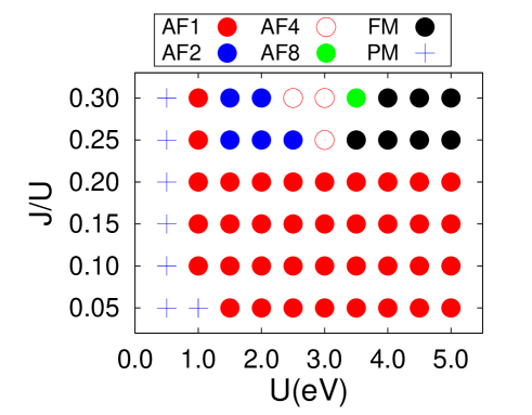
Figure 4: Phase diagram for a $16\times 1$ one-dimensional lattice, using the HF approximation at fixed $n=6.0$. The hopping amplitudes are taken from Ref. Graser08, , by truncating those hoppings to one dimension. The definition of “Paramagnetic” (PM) state is the same as in Fig. 3. The bandwidth at $U=J=0$ is $W=2.2$ eV. The notation for the many states was explained in previous figures.

With the only purpose of finding out how robust the previous results are, a real-space HF phase diagram was constructed at $n=6$ for the case of hoppings that were actually calculated in a different context, i.e. layered pnictides. Those hoppings were simply truncated to a one-dimensional chain along one of the directions of the layers. Again, there is no direct physical motivation for this portion of the calculation but merely the curiosity to gauge how different the results would be by choosing quite a different set of hopping. To our surprise, the phase diagram at $n=6$ shown in Fig. 4 is very similar to that in Fig. 3. Similarly as in Fig. 3, a paramagnetic phase exists at small $U$, a spin staggered state AF1 dominates at intermediate and large $U$ and $J/U$ not larger than 0.20, and a ferromagnetic state is stable at realistic $J/U$ and large $U$. In between, in the regime of $U/W$ between 0.5 to 1.5, approximately, a transition from AF1 to FM via intermediate Block states with an increasing size of the FM blocks is obtained. Thus, in spite of the use of quite different hoppings, the essential aspects between the phase diagrams in Figs. 3 and 4 are the same. Also at $n=5$ the physics is similar to that reported in Fig. 2 (not shown).

III.4 Electronic densities $n=5,6$ with (truncated to 2D) TlFeSe₂ hoppings

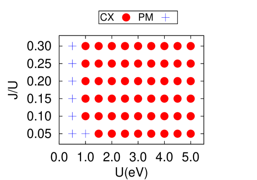
Figure 5: Magnetic phase diagram obtained using the real-space HF approximation, an $8\times 8$ two-dimensional square cluster, and working at a fixed electronic density $n=5.0$. The hopping selection was explained in the text. The explicit hopping amplitudes used for this 2D square lattice includes all the hopping matrices presented in the Appendix. The CX state is shown in Fig. 6 (b): it has staggered AFM order along the chains, supplemented by ferromagnetic coupling along the perpendicular direction with the weaker hoppings. The PM state was obtained under the same convention as in Fig. 3. The bandwidth at $U=J=0$ is $W=3.45$ eV.

As explained before, TlFeSe₂ and perhaps other quasi one-dimensional materials, appear to have a temperature range where one dimensionality prevails. However, there are small couplings in the direction perpendicular to the chain that will eventually lead to three-dimensional (3D) magnetic order at low temperatures, instead of merely power-law decaying spin correlations. Studying directly the full 3D system would be too complicated computationally, due to the rapid growth with the size of the clusters of the required CPU time and the need to have a robust linear cluster size to fit the complex spin patterns emerging in our calculations. However, an intermediate situation can be achieved if the 1D results are merely extended to two dimensions (2D) as opposed to 3D. In practice, of the vast set of hopping amplitudes obtained from the band structure calculations, those located within a single two-dimensional layer, as those shown in Fig. 11, were kept and the rest discarded. Under these circumstances, the real-space HF procedure was repeated, although this time the linear size had to be reduced to keep the computational time requirements under control. For this reason, an 8$\times$8 cluster was chosen for this portion of the study.

For the case of $n=5.0$, the phase diagram is once again dominated by a single state as it happened at this electronic density in one dimension. However, the dominant magnetic order is not a fully staggered G-type AFM state but instead a CX state with ferromagnetic order along the direction of the weak hoppings. This is conceptually interesting since it unveils deviations from a simple spin localized picture due to the presence of many orbitals and the proximity of regions with double exchange physics.

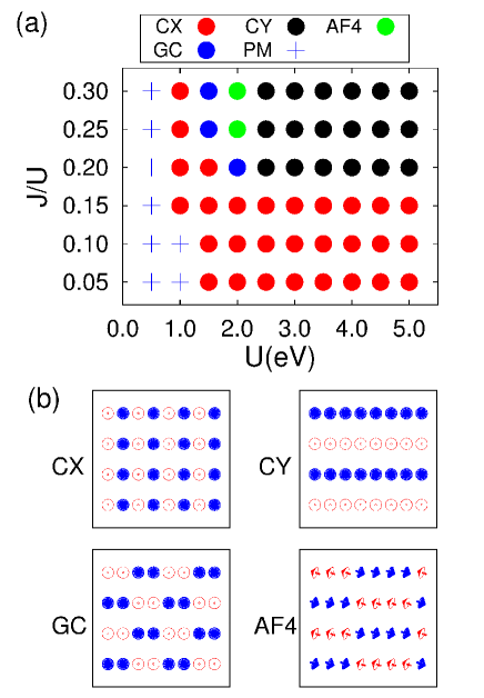
Figure 6: (a) Phase diagram obtained using the real-space HF approximation and an $8\times 8$ two-dimensional square lattice, at a fixed electronic density $n=6.0$. The hopping selection was explained in the text. The explicit hopping amplitudes used for this 2D square lattice includes all the hopping matrices presented in the Appendix section. The PM state was obtained under the same convention as in Fig. 3. The bandwidth at $U=J=0$ is $W=3.45$ eV. (b) The definition of the states used in (a). The chains direction is horizontal.

The results of this two-dimensional study for the case of $n=6.0$ are shown in Fig. 6 (a,b). As in the case of one dimension, the phase diagram is far richer at $n=6.0$ than at $n=5.0$. The phase diagram Fig. 6 still displays the small $U$ paramagnetic regime as expected, followed by the CX state for $J/U$ less than 0.20 and any $U$. This state has staggered AFM order along the 1D dominant direction, but it is FM in the direction perpendicular to the chains, as already explained for $n=5.0$. Thus, this state has C-type AFM characteristics, compatible with the tendency toward this type of states at $n$=6 in the isotropic layered two-dimensional investigations. However, at $J/U=0.20$ or larger, other states appear in the phase diagram with increasing $U$, similarly as in the previously discussed 1D cases. In particular, the FM state of 1D is replaced by the CY state, where there is ferromagnetism in the dominant chain directions, but AFM order in the perpendicular direction. This is another representative of the C-type AFM family. It is remarkable that neither the fully staggered G-AFM state nor the fully FM state are stabilized in the phase diagram in the range of couplings studied, but instead in both cases a C-AFM is stable. Finally, in between the CX and CY states, once again other complex states are stabilized, indicated as GC and AF4 in Fig. 6 (b). Here, along the chains direction these states resemble the Block states AF2 and AF4 of Fig. 3, but in the direction perpendicular the coupling is AFM (Note: the label GC is used here to match the notation employed in a recent investigation of two dimensional models varying the electronic density.luo2d In that context the GC state was found in the phase diagram and the GC label denotes a mixture of the G-AFM and C-AFM states). Perhaps due to limitations in the cluster size studied in this effort, other possible states are not present in the phase diagram, but it is possible that the size of the individual FM clusters does not stop at just 4 but a cascade of block states with increasing cluster sizes could also be stabilized (in increasingly narrower regions of parameter space) in the transition from AFM to FM states. Overall, it appears that neither fully FM nor fully staggered AFM states are stabilized, but instead the phase diagram is dominated by intermediate magnetic states such as the C-type AFM and the FM Blocks coupled AFM in both directions.

IV Density of States and Orbital Composition

After the real-space HF state is obtained via the iterative process, then a variety of observables can be calculated. In this section, the density of states (DOS) and orbital composition are provided. Figure 7 contains the DOS for $n=5.0$ in the case of the 2D cluster (see phase diagram in Fig. 5). Although the magnetic state CX that dominates the phase diagram is not spin staggered in all directions, the chains are certainly dominating since the hoppings are the largest along the direction they define. Then, it is not surprising that the staggered spin order along the chains opens a gap in the DOS similarly as it typically occurs in layered G-type AFM states.

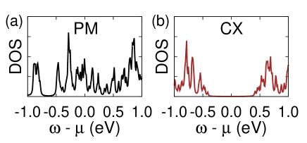
Figure 7: Density of states at representative values of couplings, corresponding to the two magnetic states shown in the 2D phase diagram corresponding to $n=5.0$ (Fig. 2). (a) PM case $U=J=0.0$; (b) CX state at $U=1.0$ and $J/U=0.25$. Increasing further $U$ results in a concomitant increase in the gap shown in panel (b).

For the case of $n=6.0$, and the concomitant phase diagram in 2D shown in Fig. 6, the DOS’s are displayed in Fig. 8. The cases (a) and (b) correspond to the paramagnetic state. Here the nonzero $U$ and $J$ in (b) induce small modifications in the relative orbital populations as compared with (a), and for this reason these panels are very similar although not identical. But in both cases a metallic state is observed as expected (albeit with low weight at the Fermi level, signaling a possible bad metal). The CX state in panel (c) is close to the border of the paramagnetic state and for this reason the gap is small of only $\sim$0.1 eV. Panel (d) contains results for the phase GC. Since in both directions electrons will have difficulty in propagating due to the staggered order, and also because $U$ is larger in panel (d) than in (c), then the gap of the GC state is larger by a factor $\sim$2 than for the CX state. A similar reasoning holds for the AF4 state shown in panel (e) with a similar gap. Finally, the CY state shown in panel (f) also has a gap of similar magnitude as the rest, in spite of the fact that panel (f) is at $U=3$ eV. The reason is that this state has ferromagnetic tendencies along the chain direction that favor metallicity, and the combination of this effect together with a robust $U$ conspire to provide a similar gap as the rest. Summarizing, in a reasonable range of values of $U$ and at the realistic $J/U=0.25$, the gaps of the many phases are approximately similar and in the range 0.1 eV to 0.2 eV.

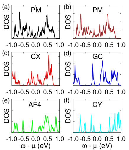
Figure 8: Density of States (DOS) at representative values of couplings, corresponding to the five magnetic states shown in the 2D phase diagram of $n=6$ (Fig. 6). (a) PM: $U=J=0.0$; (b) PM: $U=0.5$, $J/U=0.25$; (c) CX: $U=1.0$, $J/U=0.25$; (d) GC: $U=1.5$, $J/U=0.25$; (e) AF4: $U=2.0$, $J/U=0.25$; (f) CY: $U=3.0$, $J/U=0.25$.

Figure 9 contains information about the orbital composition and filling for the case of $n=5.0$ and 2D. Panel (a) shows that with increasing $U$, the population of all the five orbitals converges to 1, even though at $U=0.0$ there is an energy splitting. This is in agreement with expectations at this electronic density. At $U=1.0$ eV, panel (a) shows that still the individual orbital population is not precisely 1. Then, panel (b) does not have a sharp gap near 0.0. But with increasing Hubbard coupling, panel (c) displays a robust gap-like feature at $U=2.0$ eV for all the five curves since at this coupling all the orbitals are already in the Mott regime.

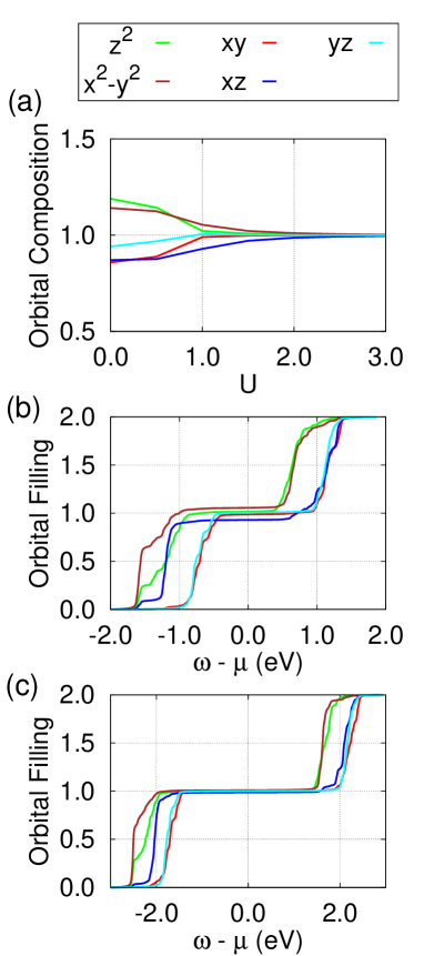
Figure 9: Orbital composition at representative values of the couplings in the 2D phase diagram corresponding to electronic density $n=5$. (a) Orbital composition vs. $U$ at fixed $J/U=0.25$; (b) Orbital fillings vs. $\omega-\mu$ at $U=1.0$ eV, and $J/U=0.25$; (c) Orbital fillings vs. $\omega-\mu$ at $U=2.0$ eV, and $J/U=0.25$.

The case of $n=6.0$ is quite different from $n=5.0$. Figure 10 (a) contains the orbital composition with increasing $U$, at $J/U=0.25$. Compatible with the ideas related with orbital selective Mott transitions,Georges in this case there are two orbitals that converge to population 1 in the range of $U$ between 1 and 2, while the rest still carry a non-integer number of electrons. As a consequence, this is a state that combines localized features related with the orbitals in the Mott state and itinerant features related with the rest of the orbitals. Previous mean-field calculations in layered 2D systems (isotropic in space) have also reported the presence of a similar orbital-selective state.previousOSMP This is also compatible with the relatively small gaps observed in the DOS at $n=6.0$ as compared with $n=5.0$. Figure 10 (b) illustrates these points once again: the two orbitals with population 1 have a robust gap signaled by the plateaux in the curve, while the rest only have a smaller gap caused by the influence of the localized spins on the itinerant carriers. Thus, the cases of $n=5.0$ and $6.0$ are fundamentally different.

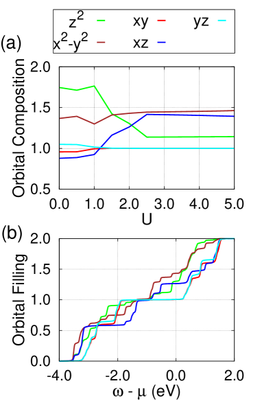
Figure 10: Orbital composition at representative values of couplings in the 2D phase diagram. (a) Orbital composition vs. $U$, at fixed $J/U=0.25$; (b) Orbital fillings vs. $\omega-\mu$ at $U=2.0$, $J/U=0.25$. The total electron filling is $n=6.0$ for both (a) and (b).

V Conclusions

In this publication, an electronic model Hamiltonian for one-dimensional iron-selenides was studied. The phase diagrams were constructed at the $3d$ iron electronic densities $n=5.0$ and $6.0$, using the numerically demanding real-space Hartree Fock approximation. The results at $n=5.0$ were obtained employing hopping amplitudes that were derived using $ab-initio$ techniques from the already synthesized material TlFeSe₂ with quasi one-dimensional structures. The $n=5.0$ phase diagram is dominated by staggered spin order along the dominant chains direction, and a robust gap in the density of states.

The case of $n=6.0$ does not correspond to any known one-dimensional selenide compound to our knowledge, thus our results have the goal of motivating experimental groups for the preparation of such a material. Our study unveils a phase diagram far richer than at $n=5.0$, particularly at the often quoted ratio $J/U=0.25$ for the iron superconductors. In this regime, the $n=6.0$ phase diagram contains a variety of novel states involving block phases with clusters of ferromagnetic spins of various lengths, antiferromagnetically coupled among them, as in recent DMRG studies by Rincón et al.rincon The density of states reveals a relatively small gap that may be indicative of a weak insulator or bad metallic behavior in a real material. Note, however, that our study was carried out employing the hopping amplitudes of the case $n=5.0$. Then, if a $n=6.0$ material is ever synthesized then the present calculations should be redone with more realistic hoppings derived from density functional theory. Nevertheless, results at $n=5.0$ also shown in our present effort indicate a weak dependence on the actual hopping set as long as a particular direction dominates, suggesting that the block states may exist in real $n=6.0$ quasi one-dimensional compounds. Considering the importance of similar unidimensional materials in the context of the cuprates together with our present analysis, all indicates that carrying out low dimensional investigations in the framework of iron selenides and pnictides may provide valuable information about the widely studied iron-based superconductors.

VI Acknowledgment

We thank Julián Rincón for useful conversations. The work of the authors was supported by the U.S. Department of Energy, Office of Basic Energy Sciences, Materials Sciences and Engineering Division.

VII Appendix

For completeness, a list of the electron hopping amplitudes between the Fe $3d$ orbitals in the $\{d_{z^{2}},d_{x^{2}-y^{2}},d_{xy},d_{xz},d_{yz}\}$ orbital basis is here provided. The matrix $t^{1j}_{[x,z]}$ describes the hopping amplitudes between $3d$ orbitals of Fe atom $1$ in the unit cell $[0,0]$ and those of Fe atom $j$ in the unit cell $[x,z]$, as shown in Fig. 11.

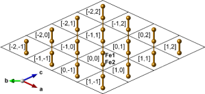
Figure 11: Schematic representation of the TlFeSe₂ crystal structure with only the Fe atoms in the $ac$ plane shown. The Fe chains run along the $-\vec{a}+\vec{c}$ direction. The shorter, 2.74 Å, (longer, 2.75 Å) NN distances between the Fe atoms are indicated by thick (thin) sticks connecting the atoms. $[x,z]$ labels the unit cells.

Matrix	TlFeSe2
$t^{11}_{[0,0]}$	$\begin{pmatrix}\textendash 0.2643&\textendash 0.0859&0&\textendash 0.0070&0\\ \textendash 0.0859&\textendash 0.3711&0&~{}~{}0.0127&0\\ 0&0&~{}~{}0.2926&0&\textendash 0.0089\\ \textendash 0.0070&~{}~{}0.0127&0&~{}~{}0.0882&0\\ 0&0&\textendash 0.0089&0&~{}~{}0.2427\end{pmatrix}$

$\begin{array}[]{l}t^{12}_{[0,0]}\\ \\ d\text{=2.74~{}\AA}\end{array}$

$\begin{pmatrix}~{}~{}0.0405&\textendash 0.2980&0&\textendash 0.2630&0\\ \textendash 0.2980&\textendash 0.2376&0&\textendash 0.4202&0\\ 0&0&\textendash 0.2253&0&\textendash 0.2593\\ \textendash 0.2630&\textendash 0.4202&0&\textendash 0.4332&0\\ 0&0&\textendash 0.2593&0&\textendash 0.2550\end{pmatrix}$

$\begin{array}[]{l}t^{12}_{[-1,1]}\\ \\ d\text{=2.75~{}\AA}\end{array}$

$\begin{pmatrix}~{}~{}0.0901&\textendash 0.2739&0&~{}~{}0.2164&0\\ \textendash 0.2739&\textendash 0.2459&0&~{}~{}0.4549&0\\ 0&0&\textendash 0.2884&0&~{}~{}0.2356\\ ~{}~{}0.2164&~{}~{}0.4549&0&\textendash 0.4450&0\\ 0&0&~{}~{}0.2356&0&\textendash 0.2156\end{pmatrix}$

$\begin{array}[]{l}t^{11}_{[-1,1]}\\ \\ d\text{=5.49~{}\AA}\end{array}$

$\begin{pmatrix}\textendash 0.0695&~{}~{}0.0184&0&\textendash 0.0128&0\\ ~{}~{}0.0062&\textendash 0.0037&0&\textendash 0.0322&0\\ 0&0&\textendash 0.0426&0&\textendash 0.0130\\ ~{}~{}0.0139&~{}~{}0.0399&0&\textendash 0.0416&0\\ 0&0&~{}~{}0.0157&0&\textendash 0.0202\end{pmatrix}$

$\begin{array}[]{l}t^{11}_{[1,-1]}\\ \\ d\text{=5.49~{}\AA}\end{array}$

$\begin{pmatrix}\textendash 0.0695&~{}~{}0.0062&0&~{}~{}0.0139&0\\ ~{}~{}0.0184&\textendash 0.0037&0&~{}~{}0.0399&0\\ 0&0&\textendash 0.0426&0&~{}~{}0.0157\\ \textendash 0.0128&\textendash 0.0322&0&\textendash 0.0416&0\\ 0&0&\textendash 0.0130&0&\textendash 0.0202\end{pmatrix}$

$\begin{array}[]{l}t^{12}_{[-1,0]}\\ \\ d\text{=5.99~{}\AA}\end{array}$

$\begin{pmatrix}\textendash 0.0601&\textendash 0.0075&\textendash 0.0004&\textendash 0.0020&\textendash 0.0001\\ \textendash 0.0075&~{}~{}0.0085&~{}~{}0.0021&\textendash 0.0047&\textendash 0.0115\\ \textendash 0.0004&~{}~{}0.0021&~{}~{}0.0152&~{}~{}0.0099&\textendash 0.0210\\ \textendash 0.0020&\textendash 0.0047&~{}~{}0.0099&\textendash 0.0029&~{}~{}0.0164\\ \textendash 0.0001&\textendash 0.0115&\textendash 0.0210&~{}~{}0.0164&\textendash 0.0521\end{pmatrix}$

$\begin{array}[]{l}t^{12}_{[0,1]}\\ \\ d\text{=5.99~{}\AA}\end{array}$

$\begin{pmatrix}\textendash 0.0601&\textendash 0.0075&~{}~{}0.0004&\textendash 0.0020&~{}~{}0.0001\\ \textendash 0.0075&~{}~{}0.0085&\textendash 0.0021&\textendash 0.0047&~{}~{}0.0115\\ ~{}~{}0.0004&\textendash 0.0021&~{}~{}0.0152&\textendash 0.0099&\textendash 0.0210\\ \textendash 0.0020&\textendash 0.0047&\textendash 0.0099&\textendash 0.0029&\textendash 0.0164\\ ~{}~{}0.0001&~{}~{}0.0115&\textendash 0.0210&\textendash 0.0164&\textendash 0.0521\end{pmatrix}$

$\begin{array}[]{l}t^{11}_{[0,-1]}\\ \\ d\text{=6.59~{}\AA}\end{array}$

$\begin{pmatrix}\textendash 0.0286&~{}~{}0.0362&\textendash 0.0083&\textendash 0.0055&\textendash 0.0197\\ \textendash 0.0075&~{}~{}0.0147&~{}~{}0.0064&~{}~{}0.0199&~{}~{}0.0265\\ \textendash 0.0527&\textendash 0.0049&\textendash 0.0048&~{}~{}0.0167&\textendash 0.0193\\ ~{}~{}0.0220&~{}~{}0.0217&\textendash 0.0156&~{}~{}0.0079&~{}~{}0.0100\\ \textendash 0.0241&~{}~{}0.0067&~{}~{}0.0094&~{}~{}0.0195&~{}~{}0.0127\end{pmatrix}$

$\begin{array}[]{l}t^{11}_{[1,0]}\\ \\ d\text{=6.59~{}\AA}\end{array}$

$\begin{pmatrix}\textendash 0.0286&~{}~{}0.0362&~{}~{}0.0083&\textendash 0.0055&~{}~{}0.0197\\ \textendash 0.0075&~{}~{}0.0147&\textendash 0.0064&~{}~{}0.0199&\textendash 0.0265\\ ~{}~{}0.0527&~{}~{}0.0049&\textendash 0.0048&\textendash 0.0167&\textendash 0.0193\\ ~{}~{}0.0220&~{}~{}0.0217&~{}~{}0.0156&~{}~{}0.0079&\textendash 0.0100\\ ~{}~{}0.0241&\textendash 0.0067&~{}~{}0.0094&\textendash 0.0195&~{}~{}0.0127\end{pmatrix}$

$\begin{array}[]{l}t^{11}_{[-1,0]}\\ \\ d\text{=6.59~{}\AA}\end{array}$

$\begin{pmatrix}\textendash 0.0286&\textendash 0.0075&~{}~{}0.0527&~{}~{}0.0220&~{}~{}0.0241\\ ~{}~{}0.0362&~{}~{}0.0147&~{}~{}0.0049&~{}~{}0.0217&\textendash 0.0067\\ ~{}~{}0.0083&\textendash 0.0064&\textendash 0.0048&~{}~{}0.0156&~{}~{}0.0094\\ \textendash 0.0055&~{}~{}0.0199&\textendash 0.0167&~{}~{}0.0079&\textendash 0.0195\\ ~{}~{}0.0197&\textendash 0.0265&\textendash 0.0193&\textendash 0.0100&~{}~{}0.0127\end{pmatrix}$

$\begin{array}[]{l}t^{11}_{[0,1]}\\ \\ d\text{=6.59~{}\AA}\end{array}$

$\begin{pmatrix}\textendash 0.0286&\textendash 0.0075&\textendash 0.0527&~{}~{}0.0220&\textendash 0.0241\\ ~{}~{}0.0362&~{}~{}0.0147&\textendash 0.0049&~{}~{}0.0217&~{}~{}0.0067\\ \textendash 0.0083&~{}~{}0.0064&\textendash 0.0048&\textendash 0.0156&~{}~{}0.0094\\ \textendash 0.0055&~{}~{}0.0199&~{}~{}0.0167&~{}~{}0.0079&~{}~{}0.0195\\ \textendash 0.0197&~{}~{}0.0265&\textendash 0.0193&~{}~{}0.0100&~{}~{}0.0127\end{pmatrix}$

$\begin{array}[]{l}t^{12}_{[1,0]}\\ \\ d\text{=8.12~{}\AA}\end{array}$

$\begin{pmatrix}~{}~{}0.0097&~{}~{}0.0150&~{}~{}0.0066&~{}~{}0.0158&\textendash 0.0061\\ ~{}~{}0.0150&\textendash 0.0150&\textendash 0.0267&\textendash 0.0127&\textendash 0.0089\\ ~{}~{}0.0066&\textendash 0.0267&\textendash 0.0609&\textendash 0.0573&\textendash 0.0130\\ ~{}~{}0.0158&\textendash 0.0127&\textendash 0.0573&\textendash 0.0272&\textendash 0.0058\\ \textendash 0.0061&\textendash 0.0089&\textendash 0.0130&\textendash 0.0058&~{}~{}0.0181\end{pmatrix}$

$\begin{array}[]{l}t^{12}_{[0,-1]}\\ \\ d\text{=8.12~{}\AA}\end{array}$

$\begin{pmatrix}~{}~{}0.0097&~{}~{}0.0150&\textendash 0.0066&~{}~{}0.0158&~{}~{}0.0061\\ ~{}~{}0.0150&\textendash 0.0150&~{}~{}0.0267&\textendash 0.0127&~{}~{}0.0089\\ \textendash 0.0066&~{}~{}0.0267&\textendash 0.0609&~{}~{}0.0573&\textendash 0.0130\\ ~{}~{}0.0158&\textendash 0.0127&~{}~{}0.0573&\textendash 0.0272&~{}~{}0.0058\\ ~{}~{}0.0061&~{}~{}0.0089&\textendash 0.0130&~{}~{}0.0058&~{}~{}0.0181\end{pmatrix}$

$\begin{array}[]{l}t^{12}_{[-2,1]}\\ \\ d\text{=8.13~{}\AA}\end{array}$

$\begin{pmatrix}~{}~{}0.0049&~{}~{}0.0123&\textendash 0.0125&\textendash 0.0034&\textendash 0.0123\\ ~{}~{}0.0123&\textendash 0.0094&~{}~{}0.0091&~{}~{}0.0130&\textendash 0.0033\\ \textendash 0.0125&~{}~{}0.0091&~{}~{}0.0074&~{}~{}0.0114&~{}~{}0.0142\\ \textendash 0.0034&~{}~{}0.0130&~{}~{}0.0114&~{}~{}0.0067&~{}~{}0.0078\\ \textendash 0.0123&\textendash 0.0033&~{}~{}0.0142&~{}~{}0.0078&\textendash 0.0002\end{pmatrix}$

$\begin{array}[]{l}t^{12}_{[-1,2]}\\ \\ d\text{=8.13~{}\AA}\end{array}$

$\begin{pmatrix}~{}~{}0.0049&~{}~{}0.0123&~{}~{}0.0125&\textendash 0.0034&~{}~{}0.0123\\ ~{}~{}0.0123&\textendash 0.0094&\textendash 0.0091&~{}~{}0.0130&~{}~{}0.0033\\ ~{}~{}0.0125&\textendash 0.0091&~{}~{}0.0074&\textendash 0.0114&~{}~{}0.0142\\ \textendash 0.0034&~{}~{}0.0130&\textendash 0.0114&~{}~{}0.0067&\textendash 0.0078\\ ~{}~{}0.0123&~{}~{}0.0033&~{}~{}0.0142&\textendash 0.0078&\textendash 0.0002\end{pmatrix}$

$\begin{array}[]{l}t^{12}_{[1,-1]}\\ \\ d\text{=8.23~{}\AA}\end{array}$

$\begin{pmatrix}~{}~{}0.0306&\textendash 0.0140&0&~{}~{}0.0156&0\\ \textendash 0.0140&~{}~{}0.0053&0&\textendash 0.0054&0\\ 0&0&~{}~{}0.0042&0&\textendash 0.0126\\ ~{}~{}0.0156&\textendash 0.0054&0&~{}~{}0.0140&0\\ 0&0&\textendash 0.0126&0&\textendash 0.0456\end{pmatrix}$

$\begin{array}[]{l}t^{12}_{[-2,2]}\\ \\ d\text{=8.24~{}\AA}\end{array}$

$\begin{pmatrix}~{}~{}0.0272&\textendash 0.0082&0&~{}~{}0.0025&0\\ \textendash 0.0082&\textendash 0.0037&0&~{}~{}0.0169&0\\ 0&0&\textendash 0.0082&0&~{}~{}0.0240\\ ~{}~{}0.0025&~{}~{}0.0169&0&~{}~{}0.0052&0\\ 0&0&~{}~{}0.0240&0&\textendash 0.0373\end{pmatrix}$

References

- (1) David C. Johnston, Adv. Phys. 59, 803 (2010), and references therein.
- (2) Pengcheng Dai, Jiangping Hu, and Elbio Dagotto, Nature Physics 8, 709 (2012).
- (3) H. Gretarsson, A. Lupascu, J. Kim, D. Casa, T. Gog, W. Wu, S. R. Julian, Z. J. Xu, J. S. Wen, G. D. Gu, R. H. Yuan, Z. G. Chen, N.-L. Wang, S. Khim, K. H. Kim, M. Ishikado, I. Jarrige, S. Shamoto, J.-H. Chu, I. R. Fisher, and Y-J. Kim, Phys. Rev. B 84, 100509(R) (2011).
- (4) T.-M. Chuang, M. P. Allan, Jinho Lee, Yang Xie, Ni Ni, S. L. Bud’ko, G. S. Boebinger, P. C. Canfield, and J. C. Davis, Science 327, 181 (2010).
- (5) T. Shimojima, F. Sakaguchi, K. Ishizaka, Y. Ishida, T. Kiss, M. Okawa, T. Togashi, C.-T. Chen, S. Watanabe, M. Arita, K. Shimada, H. Namatame, M. Taniguchi, K. Ohgushi, S. Kasahara, T. Terashima, T. Shibauchi, Y. Matsuda, A. Chainani, and S. Shin, Science 332, 564 (2011).
- (6) M. M. Qazilbash, J. J. Hamlin, R. E. Baumbach, Lijun Zhang, D. J. Singh, M. B. Maple, and D. N. Basov, Nat. Phys. 5, 647 (2009).
- (7) Rong Yu, Kien T. Trinh, Adriana Moreo, Maria Daghofer, José Riera, Stephan Haas, and Elbio Dagotto, Phys. Rev. B 79, 104510 (2009).
- (8) Qinlong Luo, George Martins, Dao-Xin Yao, Maria Daghofer, Rong Yu, Adriana Moreo, and Elbio Dagotto, Phys. Rev. B 82, 104508 (2010).
- (9) Z. P. Yin, K. Haule, and G. Kotliar, Nat. Phys. 7, 294 (2011).
- (10) Z. P. Yin, K. Haule, and G. Kotliar, Nat. Mater. 10, 932 (2011).
- (11) For a recent review see Elbio Dagotto, Rev. Mod. Phys. 85, 849 (2013).
- (12) W. Bao, Q. Huang, G. F. Chen, M. A. Green, D. M. Wang, J. B. He, X. Q. Wang, and Y. Qiu, Chinese Phys. Lett. 28, 086104 (2011).
- (13) A. Ricci, N. Poccia, G. Campi, B. Joseph, G. Arrighetti, L. Barba, M. Reynolds, M. Burghammer, H. Takeya, Y. Mizuguchi, Y. Takano, M. Colapietro, N. L. Saini, and A. Bianconi, Phys. Rev. B 84, 060511(R) (2011).
- (14) J. M. Caron, J. R. Neilson, D. C. Miller, A. Llobet, and T. M. McQueen, Phys. Rev. B 84, 180409(R) (2011).
- (15) H. Lei, H. Ryu, A. I. Frenkel, and C. Petrovic, Phys. Rev. B 84, 214511 (2011).
- (16) J. M. Caron, J. R. Neilson, D. C. Miller, K. Arpino, A. Llobet, and T. M. McQueen, Phys. Rev. B 85, 180405(R) (2012).
- (17) Y. Nambu, K. Ohgushi, S. Suzuki, F. Du, M. Avdeev, Y. Uwatoko, K. Munakata, H. Fukazawa, S. Chi, Y. Ueda, and T. J. Sato, Phys. Rev. B 85, 064413 (2012).
- (18) B. Saparov, S. Calder, B. Sipos, H. Cao, S. Chi, D. J. Singh, A. D. Christianson, M. D. Lumsden, and A. S. Sefat, Phys. Rev. B 84, 245132 (2011).
- (19) E. Dagotto, J. A. Riera, and D. J. Scalapino, Phys. Rev. 45, 5744 (1992).
- (20) E. Dagotto and T.M. Rice, Science 271, 618 (1996).
- (21) E. Dagotto, Rep. Prog. Phys. 62, 1525 (1999).
- (22) W. Li, H. Ding, P. Zhang, P. Deng, K. Chang, K. He, S. Ji, L. Wang, X. Ma, J. Wu, J.-P. Hu, Q.-K. Xue, and X. Chen, arXiv:1210.4619.
- (23) Qinlong Luo, Andrew Nicholson, Julián Rincón, Shuhua Liang, José Riera, Gonzalo Alvarez, Limin Wang, Wei Ku, German D. Samolyuk, Adriana Moreo, and Elbio Dagotto, Phys. Rev. B 87, 024404 (2013).
- (24) R. G. Veliyev, Semiconductors 45, 158 (2011), and references therein.
- (25) Z. Seidov, H.-A. Krug von Nidda, J. Hemberger, A. Loidl, G. Sultanov, E. Kerimova, and A. Panfilov, Phys. Rev. B 65, 014433 (2001), and references therein.
- (26) W. Bronger, A. Kyas, and P. Müller, Journal of Solid State Chemistry 70, 262 (1987).
- (27) D. Welz and M. Nishi, Phys. Rev. B 45, 9806 (1992), and references therein.
- (28) B. J. Kim, H. Koh, E. Rotenberg, S.-J. Oh, H. Eisaki, N. Motoyama, S. Uchida, T. Tohyama, S. Maekawa, Z.-X. Shen, and C. Kim, Nat. Physics 2, 397 (2006), and references therein.
- (29) J. Schlappa, K. Wohlfeld, K. J. Zhou, M. Mourigal, M. W. Haverkort, V. N. Strocov, L. Hozoi, C. Monney, S. Nishimoto, S. Singh, A. Revcolevschi, J.-S. Caux, L. Patthey, H. M. Rxnnow, J. van den Brink and T. Schmitt, Nature 485, 82 (2012), and references therein.
- (30) P. Blaha, K. Schwarz, G. K. H. Madsen, D. Kvasnicka, and J. Luitz, WIEN2k, An Augmented PlaneWave+LocalOrbitals Program for Calculating Crystal Properties (Karlheinz Schwarz, Techn. Universität Wien, Austria, 2001).
- (31) J. P. Perdew, K. Burke and M. Ernzerhof, Phys. Rev. Lett. 77 3865 (1996).
- (32) M. Aichhorn et al. Phys. Rev. B, 80, 085101 (2009).
- (33) J. P. Perdew and A. Zunger, Phys. Rev. B 23, 5048 (1981).
- (34) P. Giannozzi, S. Baroni, et al J. of Phys. Cond. Matt. 21, 395502 (2009).
- (35) D. Vanderbilt, Phys. Rev. B 41, 7892 (1990).
- (36) A. M. Rappe, K. M. Rabe, E. Kaxiras, and J. D. Joannopoulos, Phys. Rev. B 41, 1227 (1990).
- (37) I. Souza, N. Marzari, and D. Vanderbilt, Phys. Rev. B 65, 035109 (2001).
- (38) A. A. Mostofi, J. R. Yates, Y.-S. Lee, I. Souza, D. Vanderbilt, N. Marzari, Comput. Phys. Commun. 178, 685 (2008).
- (39) Kurt Klepp and Herbert Boller, Monatshefte für Chemie 110, 1045–1055 (1979).
- (40) S. Graser, T. A. Maier, P. J. Hirschfeld, and D. J. Scalapino, New J. Phys. 11, 025016 (2009).
- (41) Yogesh Singh, M. A. Green, Q. Huang, A. Kreyssig, R. J. McQueeney, D. C. Johnston, and A. I. Goldman, Phys. Rev. B 80, 100403(R) (2009), and references therein.
- (42) J. Lamsal, G. S. Tucker, T. W. Heitmann, A. Kreyssig, A. Jesche, Abhishek Pandey, Wei Tian, R. J. McQueeney, D. C. Johnston, and A. I. Goldman, Phys. Rev. B 87, 144418 (2013), and references therein.
- (43) Julián Rincón, Adriana Moreo, Gonzalo Alvarez, and Elbio Dagotto, Phys. Rev. Lett. 112, 106405 (2014).
- (44) Qinlong Luo and Elbio Dagotto, Phys. Rev. B 89, 045115 (2014).
- (45) A. Georges, L. de’ Medici, and J. Mravlje, Annu. Rev. Cond. Mat. Phys. 4, 137 (2013), and references therein.
- (46) R. Yu and Q. Si, Phys. Rev. B 86, 085104 (2012); R. Yu and Q. Si, Phys. Rev. Lett. 110, 146402 (2013); E. Bascones, B. Valenzuela, and M. J. Calderón, Phys. Rev. B 86, 174508 (2012); B. Valenzuela, M. J. Calderón, G. León, E. Bascones, Phys. Rev. B 87, 075136 (2013).