UCB-PTH-14/07

Grand Unification, Axion, and Inflation in
Intermediate Scale Supersymmetry

Lawrence J. Hall, Yasunori Nomura, and Satoshi Shirai

Berkeley Center for Theoretical Physics, Department of Physics,
and Theoretical Physics Group, Lawrence Berkeley National Laboratory,
University of California, Berkeley, CA 94720, USA

1 Introduction

The key discovery from the first run of the Large Hadron Collider (LHC) is a highly perturbative Higgs boson coupled with no sign of any new physics that would allow a natural electroweak scale. Remarkably, the value of the Higgs mass implies that the Standard Model (SM) remains perturbative to very high energy scales. Although this “Lonely Higgs” picture could easily be overturned by discoveries at the next run of the LHC, at present we are confronted with a very surprising situation. A variety of new physics possibilities was introduced in the 1970s and 1980s yielding a standard paradigm of a natural weak scale that was almost universally accepted. While the absence of new physics at LEP and elsewhere led to doubts about naturalness, the Lonely Higgs discovery at LHC warrants new thinking on the naturalness of the weak scale and the likely mass scale of new physics.

An intriguing feature of the Lonely Higgs discovery is that the Higgs quartic coupling, on evolution to high energies, passes through zero and then remains close to zero up to unified scales, providing evidence for a highly perturbative Higgs sector at high energies. This closeness to zero of the quartic coupling cannot be explained by the SM, and hence is a guide in seeking new physics at very high scales. The Higgs boson mass was predicted to be in the range $\approx(128-141)~{}{\rm GeV}$ from a supersymmetric boundary condition at unified energies [1]. Furthermore, it was pointed out that in such theories $\tan\beta$ near unity can result naturally, leading to a Higgs mass prediction of $(128\pm 3)~{}{\rm GeV}$, with the central value gradually decreasing as the scale of supersymmetry is lowered below the unified scale. After the Higgs boson discovery, the connection between supersymmetry at a high scale and the Higgs mass was investigated further [2, 3].

In a previous paper [4], two of us introduced Intermediate Scale Supersymmetry (ISS) to explain two key observations

• The SM quartic coupling, when evolved to large scales, passes through zero at $\mu_{c}$. This can be accounted for by taking the SM superpartner mass scale $\tilde{m}\sim\mu_{c}$. From Fig. 1(a), $\mu_{c}\sim 10^{9}~{}\mbox{--}10^{13}~{}{\rm GeV}$ at 1-$\sigma$ (allowing for the possibility of a TeV-scale wino for dark matter).

• States of a minimal supersymmetric grand unified theory at $\tilde{m}$ can account for precision gauge coupling unification.

In addition to these, in this paper we study ISS models that have a third key feature

• Below the cutoff scale of the theory $\Lambda$, which is likely close to the Planck mass, the theory possesses only a single mass scale, $\tilde{m}$.

In this paper we study two different aspects of ISS. In Section 3, we pursue a class of ISS models that lead more cleanly to the vanishing of the quartic coupling near $\tilde{m}$, have a new proton decay signal and are more elegant. In Section 4, we argue that in ISS the mass scale $\tilde{m}$ may be identified with one or more key mass scales of new physics: the axion decay constant, the energy scale of inflation, and the seesaw scale for neutrino masses.

ISS provides a unifying theme to the diverse physics that we discuss, since it is all triggered by the same underlying mass scale. The scale $\tilde{m}$ directly gives the superpartner masses and can also be the origin of the axion decay constant, inflation, and right-handed neutrino masses. Within this framework, the scale of weak interactions and of the Grand Unified Theory (GUT) need some explanation.

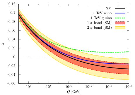
(a) Higgs quartic coupling $\lambda$

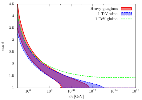
(b) 1-$\sigma$ band of $\tan\beta$

Figure 1: (a) The renormalization group running of the Higgs quartic coupling $\lambda$ for the SM (solid black line, with 1-$\sigma$ and 2-$\sigma$ regions from uncertainties of the experimental input parameters indicated by dark and light shades, respectively) and for the $1~{}{\rm TeV}$ wino (solid blue) and gluino (dashed green) in addition to the SM particles. (b) The value of $\tan\beta$ required to reproduce the observed Higgs boson mass as a function of the superpartner mass scale $\tilde{m}$ in the case that the theory below $\tilde{m}$ is the SM (red region bounded by solid lines), the SM with $1~{}{\rm TeV}$ wino (blue region bounded by dashed lines), and the SM with $1~{}{\rm TeV}$ gluino (dashed green line). The regions for the first two cases correspond to the 1-$\sigma$ uncertainties for the input experimental parameters.

In ISS the weak scale is highly fine-tuned, for example by twenty orders of magnitude for $\tilde{m}=10^{12}~{}{\rm GeV}$, and can be understood in the multiverse, which provides a coherent framework for understanding both the fine-tuning of the weak scale and the cosmological constant [5, 6]. In the $SU(5)$ unified model introduced in this paper, the fields responsible for weak breaking, $H,\bar{H}$, and $SU(5)$ breaking, $\Sigma$, do not have supersymmetric mass terms and are massless in the supersymmetric flat-space limit. Once supersymmetry is broken and the cosmological constant is fine-tuned, supergravity interactions induce an effective superpotential

$$W_{\rm eff}\sim\tilde{m}\times\left(\Sigma^{2},\;H\bar{H},\;\frac{1}{\Lambda}\Sigma^{3},\;\frac{1}{\Lambda}H\Sigma\bar{H},\;...\right).$$ (1)

This yields an $SU(5)$ breaking vacuum $\langle\Sigma\rangle\sim O(\Lambda)$, and we choose order unity coefficients so that this vacuum expectation value (VEV) is somewhat less than $\Lambda$. The heavy $XY$ gauge supermultiplet lies just below $\Lambda$, while all other states in $H,\bar{H},\Sigma$ have masses of order $\tilde{m}$. These states make a significant contribution to gauge coupling unification, and the color triplet states in $H,\bar{H}$ yield an interesting proton decay signal.

The $H\Sigma\bar{H}$ coupling is of order $\tilde{m}/\Lambda$, and hence leads to a negligible contribution to the Higgs quartic, which is dominated by the electroweak gauge contribution: $\lambda(\tilde{m})\simeq 0.03\,(\tan^{2}\!\beta-1)^{2}$ for $|\tan^{2}\!\beta-1|\ll 1$, where $\lambda$ is normalized such that $V(h)\supset(\lambda/2)(h^{\dagger}h)^{2}$, and the angle $\beta$ defines the combination of Higgs doublets that is fine-tuned light to become the SM Higgs. A value of $\tan^{2}\!\beta$ in the range of about $0.5$ to $2$ is sufficient to understand a small value of $\lambda(\tilde{m})$; however, in the limit that the Higgs mixing parameter (the Higgsino mass) $\mu$ becomes larger than $\tilde{m}$, $\tan^{2}\!\beta-1\sim O(\tilde{m}^{2}/\mu^{2})$, so that $\lambda(\tilde{m})$ rapidly drops below $0.01$.

The organization of the rest of the paper is as follows. In Section 2 we closely examine the running of the Higgs quartic coupling in the SM, and with the addition of a TeV-scale wino, to determine the range of $\mu_{c}$. In Section 3 we introduce and study a specific simple $SU(5)$ GUT that is representative of a class of grand unified theories that have just a single mass scale, $\tilde{m}$. We study the spectrum, dark matter, gauge coupling unification and proton decay in this model. In Section 4 we argue that in ISS other fundamental physics may be linked to the scale $\tilde{m}$, in particular, neutrino masses, axions, and inflation. Finally we summarize in Section 5.

2 Higgs Quartic Coupling and ISS

Before entering into the main part of the paper, in this section we discuss the scale of supersymmetry breaking suggested by the current experimental data within the ISS framework. In Fig. 1(a), we show the running of the $\overline{\rm MS}$ Higgs quartic coupling $\lambda$ in the SM as a function of the renormalization scale $Q$ (solid, black line). Here, the dark and light shaded regions correspond to the 1-$\sigma$ and 2-$\sigma$ ranges for the experimental input parameters, respectively, for which we have used $m_{t}=173.34(76)~{}{\rm GeV}$ [7], $m_{h^{0}}=125.40(45)~{}{\rm GeV}$ [8, 9], $m_{W}=80.367(7)~{}{\rm GeV}$, $m_{Z}=91.1875(21)~{}{\rm GeV}$ [10], and $\alpha_{3}(m_{Z})=0.1184(7)$ [11]. The figure also shows the running of $\lambda$ in the cases that the wino and gluino exist at $1~{}{\rm TeV}$ in addition to the SM particles (solid blue and dashed green lines, respectively). In drawing these lines/regions, we have used, following Ref. [12], 2-loop (1-loop) threshold corrections and 3-loop (2-loop) renormalization group equations for the SM particles (the wino and gluino). As can be seen from the figure, $\lambda$ crosses zero at an intermediate scale $\mu_{c}\sim 10^{9}\mbox{--}10^{13}~{}{\rm GeV}$ for the SM, although uncertainties from experimental input parameters are still very large. The situation is similar if there is a wino at $1~{}{\rm TeV}$ (which is not entirely trivial as the crossing scale is highly sensitive to physics at lower energies as can be seen in the case in which the gluino exists at $1~{}{\rm TeV}$).

In the rest of the paper, we assume that the Higgs quartic coupling indeed crosses zero at $\mu_{c}$ if we evolve it to higher energy scales using the SM renormalization group equations (or those with a TeV-scale wino), although the possibility of the crossing scale being around the unification/Planck scale $\sim 10^{16}~{}\mbox{--}~{}10^{18}~{}{\rm GeV}$ is not yet excluded if we allow 2- to 3-$\sigma$ ranges for the current experimental errors. As discussed above and in Ref. [4], we identify this scale to be the scale for the superpartner masses $\tilde{m}$, at which the supersymmetric standard model (together with a part of the GUT particles) is reduced to the SM (possibly together with a wino or Higgsino) at lower energies. Since $\lambda\ll 1$ at this scale, this implies $\tan\beta\sim 1$. In Fig. 1(b), we show the value of $\tan\beta$ needed to reproduce the observed Higgs boson mass $m_{h^{0}}\simeq 125~{}{\rm GeV}$ as a function of the superpartner mass scale. Here, we have assumed that all the scalar superpartners have common mass $\tilde{m}$; the gaugino and Higgsino masses are also taken to be $\tilde{m}$ and the scalar trilinear $A$-terms are set to be zero. We find that for the cases of the SM and the SM with a TeV-scale wino, the superpartner masses must be at an intermediate scale:

$$\tilde{m}\sim 10^{9}\mbox{--}10^{13}~{}{\rm GeV},$$ (2)

for $\tan\beta\sim 1$ at the 1-$\sigma$ level. As can be seen from the figure, and emphasized in Ref. [4], this conclusion does not require $\tan\beta$ to be extremely close to $1$. Indeed, for $0.5\lesssim\tan^{2}\!\beta\lesssim 2$, the range of the superpartner masses suggested by the central values for the experimental data is still close to Eq. (2), and there is a wide range of parameter space which leads to these values of $\tan\beta$. (In fact, even values of $\tan\beta$ very close to $1$ can naturally be obtained if $\mu$ is somewhat larger than $\tilde{m}$.) Below, we will use values of $\tilde{m}$ in Eq. (2) as our guide in discussing ISS theories.

In this paper, we mostly assume that supersymmetry breaking is mediated to the GUT sector (the sector charged under the SM gauge group) at a high scale $M_{*}$ close to the UV cutoff scale $\Lambda$ of the unified theory, which we expect to be within an order of magnitude of the reduced Planck scale $M_{\rm Pl}\simeq 2.4\times 10^{18}~{}{\rm GeV}$: $M_{*}\sim\Lambda\sim M_{\rm Pl}$. We then find that the gravitino mass $m_{3/2}=F/\sqrt{3}M_{\rm Pl}$ is roughly the same order of magnitude as $\tilde{m}\sim F/M_{*}$, where $F$ is the $F$-term VEV of the supersymmetry breaking field. In this paper we do not discriminate the sizes of the two, and treat them to be of the same order: $m_{3/2}\sim\tilde{m}$.

3 ISS with Intermediate Scale Colored Higgses

In this section, we present a simple model of ISS. It is representative of a class of ISS GUTs where the only scale below the cutoff is that of supersymmetry breaking. The model presented here differs from the one in Ref. [4] in that the mass of the whole $H({\bf 5})+\bar{H}({\bf 5}^{*})$ Higgs fields, of which the SM Higgs field is a part, now arises from supersymmetry breaking, where the numbers in parentheses denote representations under the $SU(5)$ GUT group. This is achieved in a simple manner by obtaining the whole Higgs potential, including the one associated with the GUT-breaking field $\Sigma({\bf 24})$, from the Kähler potential. We first describe the model and spectrum, discussing if/when the wino mass is lowered to the TeV scale due to a cancellation among various contributions as a result of environmental selection associated with the dark matter abundance. We then discuss gauge coupling unification and proton decay. We also present a detailed phenomenological analysis of the model in the case that the supersymmetry breaking parameters obey the mSUGRA-like boundary conditions at the supersymmetry breaking mediation scale $M_{*}$.

3.1 Model

We consider that physics below the cutoff scale $\Lambda\sim M_{\rm Pl}$ is well described by a supersymmetric GUT with the same field content as the minimal supersymmetric $SU(5)$ GUT. The matter content of the model consists of the $\Sigma({\bf 24})$, $H({\bf 5})$, and $\bar{H}({\bf 5}^{*})$ Higgs fields as well as three generations of the matter fields $T({\bf 10})$ and $\bar{F}({\bf 5}^{*})$, where we have suppressed the generation indices. (Right-handed neutrino superfields $N({\bf 1})$’s will be introduced in Section 4 when we discuss neutrino masses.)

As in Ref. [4], we consider that the potential for the GUT-breaking field $\Sigma$ arises from the Kähler potential:

$$K\supset\frac{c_{2}}{2}\Sigma^{2}+\frac{c_{3}}{3\Lambda}\Sigma^{3}+{\rm h.c.},$$ (3)

where $c_{2,3}$ are dimensionless couplings of order unity, while $\Lambda\sim M_{\rm Pl}$ is the UV cutoff of the unified theory. Similarly, here we also consider that the potential associated with the $H,\bar{H}$ Higgs fields arises from the Kähler potential terms

$$K\supset d_{2}H\bar{H}+\frac{d_{3}}{\Lambda}H\Sigma\bar{H}+{\rm h.c.},$$ (4)

where $d_{2,3}$ are dimensionless couplings of order unity. We assume that there is no interaction in the superpotential corresponding to the terms in Eqs. (3, 4) at the fundamental level (i.e. in the supersymmetric flat-space limit). This can be achieved, e.g., if the theory possesses an $R$ symmetry under which $\Sigma$ and $H\bar{H}$ are neutral:

$$\Sigma(0),\qquad H\bar{H}(0).$$ (5)

When supersymmetry is broken and the cosmological constant is fine-tuned, the Kähler potential interactions of Eqs. (3, 4) yield the effective superpotential through supergravity effects [14]:

$$W_{\rm eff}=\frac{m_{\Sigma}}{2}\Sigma^{2}+\frac{\lambda_{\Sigma}}{3}\Sigma^{3}+\frac{m_{H}}{2}H\bar{H}+\lambda_{H}H\Sigma\bar{H},$$ (6)

where $m_{\Sigma}=c_{2}m_{3/2}^{*}$, $\lambda_{\Sigma}=c_{3}m_{3/2}^{*}/\Lambda$, $m_{H}=d_{2}m_{3/2}^{*}$, and $\lambda_{H}=d_{3}m_{3/2}^{*}/\Lambda$, so that

$$m_{\Sigma},\,m_{H}\sim O(\tilde{m}),\qquad\lambda_{\Sigma},\,\lambda_{H}\sim O\Bigl{(}\frac{\tilde{m}}{\Lambda}\Bigr{)}.$$ (7)

Here, we have used $m_{3/2}\sim\tilde{m}$. The first two terms of Eq. (6) provide a non-zero VEV of $\Sigma$, $\langle\Sigma\rangle\sim m_{\Sigma}/\lambda_{\Sigma}\sim O(\Lambda)$, breaking $SU(5)$ to the SM gauge group. In general, supersymmetry breaking effects in the $\Sigma$ potential lead to an $O(1)$ shift of the $\Sigma$ VEV, giving a VEV for the $F$-component of $\Sigma$ of order $\tilde{m}\Lambda$:

$$\langle\Sigma\rangle\sim O(\Lambda),\qquad F_{\Sigma}\sim O(\tilde{m}\Lambda).$$ (8)

We take parameters of the model such that $\langle\Sigma\rangle$ is parametrically, e.g. a factor of a few to an order of magnitude, smaller than $\Lambda$, to ensure that there is an energy interval below $\Lambda$ in which physics is described by the $SU(5)$ theory.

Below the energy scale $\langle\Sigma\rangle$, which we will see is determined from gauge coupling unification as

$$\langle\Sigma\rangle\sim 10^{16}\mbox{--}10^{17}~{}{\rm GeV},$$ (9)

the massive vector supermultiplets containing the GUT gauge bosons decouple, and physics is well described by the low-energy supersymmetric gauge theory with the SM gauge group $SU(3)_{\rm C}\times SU(2)_{\rm L}\times U(1)_{\rm Y}$. An important property of the superpotential in Eq. (6) with Eq. (7) is that because of the overall $\tilde{m}$ factor, the masses of the uneaten components of $\Sigma$—$\Sigma_{8}({\bf 8},{\bf 1})_{0}$, $\Sigma_{3}({\bf 1},{\bf 3})_{0}$, and $\Sigma_{1}({\bf 1},{\bf 1})_{0}$ where the numbers represent the SM gauge quantum numbers—are at the intermediate scale:

$$M_{\Sigma_{8}}\sim M_{\Sigma_{3}}\sim M_{\Sigma_{1}}\sim O(\tilde{m}),$$ (10)

where superpartners of the Supersymmetric Standard Model (SSM) exist [4]. This potentially has cosmological implications. For example, if the Hubble parameter during inflation is large $H_{I}>\tilde{m}$, as suggested by the recent BICEP2 observation [16], then depending on the dynamics during inflation (e.g. the sign of the Hubble induced mass-squared for $\Sigma$), the GUT symmetry may be recovered during inflation, which would lead to unwanted monopole production after inflation. Below, we assume that such symmetry recovery does not occur.

In a similar manner, in the present model the masses of the colored Higgs fields, as well as those of the second Higgs doublet $H_{D}$ and Higgsino $\tilde{h}$ of the SSM, are also at the intermediate scale. In the minimal $SU(5)$ GUT, the doublet Higgses $H_{u}$ and $H_{d}$ of the SSM are embedded in the fundamental representations of $SU(5)$ as $H=(H_{u},H_{C})$ and $\bar{H}=(H_{d},\bar{H}_{C})$. The superpotential of Eq. (6) implies that the masses for all these fields are also of order $\tilde{m}$:

$$M_{H_{C}}\sim M_{H_{D}}\sim M_{\tilde{h}}\sim O(\tilde{m}),$$ (11)

except for the light Higgs doublet $h$ of the SM, which is environmentally selected to be of order the weak scale $v\ll\tilde{m}$. One might think that such low values for the colored Higgs masses are excluded by the proton decay constraints. This is, however, not the case as will be discussed in Section 3.4. In Fig. 2, we give a schematic depiction of the spectrum of the present model. In the figure, we have put the wino, $\tilde{W}$, to be at a TeV scale, since its mass may be environmentally selected to be in this range; see Section 3.2 below.

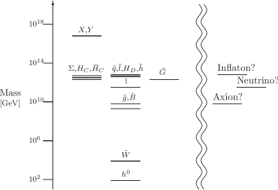
Figure 2: A schematic depiction of the spectrum of the model. Here, $X,Y$ represent the massive GUT gauge supermultiplets, $\Sigma$ uneaten components of the $\Sigma({\bf 24})$ superfield, and $H_{C}$ and $\bar{H}_{C}$ the colored Higgs supermultiplets; the other symbols denote particles in the SSM in the self-explanatory notation (with $\tilde{G}$ being the gravitino). We have depicted the wino, $\tilde{W}$, at a TeV scale, although it may be at the intermediate scale $\tilde{m}$ if the reheating temperature after inflation is sufficiently low or $R$-parity is broken; see discussions in Section 3.2. The scale $\tilde{m}$ can lead to neutrino masses, inflation, and axions, as indicated on the right.

There are several virtues in the model presented here, with the last two terms in Eq. (6) arising from the Kähler potential, compared to the model in Ref. [4], in which these terms exist in the superpotential before supersymmetry breaking with $m_{H}\sim O(\langle\Sigma\rangle)$ and $\lambda_{H}\sim O(1)$. First, since the supersymmetric masses of $\Sigma_{3}$ and $\Sigma_{1}$ are comparable to $\tilde{m}$, the interaction $\lambda_{H}H\Sigma\bar{H}$ in the superpotential gives a non-decoupling contribution to the Higgs quartic coupling: $\delta\lambda\sim\lambda_{H}^{2}\sin^{2}2\beta$. In order to preserve the identification of $\tilde{m}$ to be at a scale close to the point in which $\lambda$ crosses zero, as in Eq. (2), this contribution needs to be small, $\lambda_{H}\lesssim 0.1$. In the model of Ref. [4], this condition needs to be imposed by hand, while here it is automatic because $\lambda_{H}\sim O(\tilde{m}/\Lambda)\ll 1$. Note that since $m_{H}\sim O(\tilde{m})$ and $\lambda_{H}\sim O(\tilde{m}/\Lambda)$, the present model does not require doublet-triplet splitting (except for the fine-tuning needed to make the SM Higgs light); namely, the contributions to the mass of the heavy Higgs doublet from the third and fourth terms in Eq. (6) need not be nearly canceled with each other. This allows us to have a natural size of $F_{\Sigma}\sim O(\tilde{m}\Lambda)$ in Eq. (8) while still allowing for successful electroweak symmetry breaking, since it only leads to the holomorphic supersymmetry-breaking mass for the Higgs doublets of order $\mu B\approx\lambda_{H}F_{\Sigma}\sim O(\tilde{m}^{2})$. (In the model of Ref. [4], $F_{\Sigma}\sim O(\tilde{m}\Lambda)$ leads to a too large $\mu B$ term of order $\tilde{m}\Lambda$, so that $F_{\Sigma}$ must be suppressed by extra environmental selection.) Finally, the fact that $m_{H}\sim O(\tilde{m})$ implies that the level of fine-tuning needed to reproduce electroweak symmetry breaking is of order $v^{2}/\tilde{m}^{2}$ in the present model, while the one in Ref. [4] requires an extra factor of order $\tilde{m}^{2}/\Lambda^{2}$ to keep $\mu^{2}$ and $\mu B$ to be of order $\tilde{m}^{2}$. While none of the above issues excludes the model in Ref. [4], their absence adds an aesthetic appeal to the model discussed here.

The electroweak symmetry is broken by the VEV of the light SM Higgs doublet $h$, whose mass-squared parameter (and thus VEV) is fine-tuned to be of order the weak scale due to environmental selection. Specifically, the mass-squared matrix for the two Higgs doublets at the scale $\tilde{m}$ is given by

$${\cal M}_{\rm H}^{2}=\begin{pmatrix}|\mu|^{2}+m_{H_{u}}^{2}&\mu B\\ \mu B&|\mu|^{2}+m_{H_{d}}^{2}\end{pmatrix},$$ (12)

where $|\mu|^{2}$, $|\mu B|$, $|m_{H_{u}}^{2}|$, $|m_{H_{d}}^{2}|$ are of order $\tilde{m}^{2}$. These parameters are chosen such that one Higgs doublet remain below $\tilde{m}$, i.e. the determinant of the matrix ${\cal M}_{\rm H}^{2}$ to be extremely small compared with its natural size $\sim\tilde{m}^{4}$. The resulting SM Higgs doublet is given by the combination $h\approx\sin\beta\,h_{u}+\cos\beta\,h_{d}^{\dagger}$ with

$$\tan^{2}\!\beta=\frac{|\mu|^{2}+m_{H_{d}}^{2}}{|\mu|^{2}+m_{H_{u}}^{2}}.$$ (13)

Since the quartic coupling for the Higgs is given by

$$\lambda(\tilde{m})=\frac{g^{2}+g^{\prime 2}}{4}\,\cos^{2}\!2\beta,$$ (14)

where $g$ and $g^{\prime}$ are the $SU(2)_{\rm L}$ and $U(1)_{\rm Y}$ gauge couplings at $\tilde{m}$, we consider $\tan\beta\sim 1$. Such values of $\tan\beta$ are easily obtained, e.g., if $|\mu|^{2}\gtrsim|m_{H_{u},H_{d}}^{2}|$ or if $m_{H_{u}}^{2}$ and $m_{H_{d}}^{2}$ are nearly degenerate; see also the discussion in Section 3.5. With electroweak symmetry breaking, the SM quarks and leptons obtain masses through the standard Yukawa interactions in the superpotential

$$W=y_{U}TTH+y_{D}T\bar{F}\bar{H}+\frac{\eta_{U}}{\Lambda}\Sigma TTH+\frac{\eta_{D}}{\Lambda}\Sigma T\bar{F}\bar{H}+\cdots,$$ (15)

where we have suppressed the generation indices. Higher-dimension terms involving $\Sigma$ are needed to correct unwanted $SU(5)$ relations for the quark/lepton masses.

To summarize, the model is characterized by the following holomorphic part of the Kähler potential, $\tilde{K}$, and superpotential, $W$:

$$\tilde{K} =\Lambda^{2}\,f\Bigl{(}\frac{\Sigma}{\Lambda},\frac{H\bar{H}}{\Lambda^{2}}\Bigr{)},$$ (16)

$$W =y_{U}\Bigl{(}\frac{\Sigma}{\Lambda}\Bigr{)}\,TTH+y_{D}\Bigl{(}\frac{\Sigma}{\Lambda}\Bigr{)}\,T\bar{F}\bar{H},$$ (17)

(except for the terms needed for neutrino masses; see Section 4.1), where $f$ is a holomorphic function with the coefficients expected to be of order unity, and $y_{U}$ and $y_{D}$ are holomorphic functions associated with the Yukawa couplings. Here, we have assumed $R$-parity. The form of Eqs. (16, 17), including $R$ parity conservation, can be easily enforced by an $R$ symmetry; for example, we may assign a neutral $R$ charge to $\Sigma$, $H$, and $\bar{H}$, as in Eq. (5), and a unit charge to $T$ and $\bar{F}$. (A different charge assignment will be considered in Section 4.1.) All the dimensionful parameters, except $\Lambda$, are generated through supersymmetry breaking $\tilde{m}$, leading to the effective superpotential of Eq. (6). The GUT symmetry is broken at $\langle\Sigma\rangle\sim O(\Lambda)$, while the electroweak symmetry—due to environmental selection—at $\langle h\rangle=v\ll\tilde{m}$.

We finally discuss the gaugino masses. Unlike scalar superpartners, the gaugino masses may be protected against supersymmetry breaking effects via some symmetry. For example, if the supersymmetry breaking field $X$ has some charge, its direct coupling to the gauge field-strength superfields $[X{\cal W}^{\alpha}{\cal W}_{\alpha}/\Lambda]_{\theta^{2}}$ is suppressed. There are, however, many other sources for the gaugino masses: anomaly mediation [17], threshold corrections from $H$ and/or $\Sigma$, and the higher dimension operator $[\Sigma{\cal W}^{\alpha}{\cal W}_{\alpha}/\Lambda]_{\theta^{2}}$ with $F_{\Sigma}\neq 0$. In particular, since the operator $[\Sigma{\cal W}^{\alpha}{\cal W}_{\alpha}/\Lambda]_{\theta^{2}}$ is used to reproduce the observed SM gauge couplings (see Section 3.3) and we naturally expect $F_{\Sigma}\sim O(\tilde{m}\Lambda)$ (see Eq. (8)), the last contribution gives typically the gaugino masses not much smaller than $\tilde{m}$. As we will see in the next subsection, however, the wino mass may have to be lowered to a TeV scale as a result of environmental selection associated with dark matter. This occurs through a cancellation of various contributions given above, which in turn could suppress the gluino and bino masses through GUT relations. Note that the cancellation of the wino mass requires a modest suppression of $F_{\Sigma}$ and/or the coefficient of $[\Sigma{\cal W}^{\alpha}{\cal W}_{\alpha}/\Lambda]_{\theta^{2}}$ to allow the cancellation of its contribution with the rest, which are one-loop suppressed. We thus expect that the gaugino masses are in the range

$$M_{\lambda}\approx O(10^{-2}\mbox{--}1)\,\tilde{m},$$ (18)

except possibly for the wino, which may be at a TeV scale.

3.2 TeV-scale wino

If $R$-parity is unbroken, the lightest supersymmetric particle (LSP) is stable and contributes to the dark matter once cosmologically produced. The abundance of the LSP in the universe may depend strongly on the reheating temperature $T_{R}$ after inflation as well as the branching ratio of the inflaton decay into the LSP. Here we see that this most likely requires the mass of the LSP, $m_{\rm LSP}$, to be in the TeV region. Such a small LSP mass may result from a cancellation of various contributions as a result of environmental selection associated with dark matter [18].

Let us first consider the case in which $T_{R}\gtrsim m_{\rm LSP}$. In this case, the LSP is thermalized and its abundance is roughly given by

$$\Omega^{\rm th}h^{2}\sim 10^{16}\left(\frac{m_{\rm LSP}}{10^{12}~{}{\rm GeV}}\right)^{2}.$$ (19)

This grossly overcloses the universe for $m_{\rm LSP}\sim O(\tilde{m})$. We now consider the case $T_{R}\ll m_{\rm LSP}$. In this case, thermal gas scattering and inflaton decay may still lead to a significant amount of the LSP abundance. From thermal scattering, we obtain the approximate LSP abundance of

$$\Omega^{\rm sc}h^{2}\sim 10^{21}\left(\frac{T_{R}}{m_{\rm LSP}}\right)^{7}.$$ (20)

(A similar estimate in a different context can be found in Ref. [19].) Furthermore, if the mass of the inflaton $m_{\phi}$ is sufficiently larger than $m_{\rm LSP}$, the inflaton may directly decay into LSPs which do not effectively annihilate afterwards. The resulting LSP abundance is then roughly given by

$$\Omega^{\rm dec}h^{2}\sim 10^{20}\,B_{\phi}\left(\frac{T_{R}}{m_{\phi}}\right)\left(\frac{m_{\rm LSP}}{10^{12}~{}{\rm GeV}}\right),$$ (21)

where $B_{\phi}$ is the branching fraction of the inflaton decay to the LSP. We thus find that unless $T_{R}\lesssim 10^{-3}\,m_{\rm LSP}$ and $B_{\phi}$ is essentially zero, the LSP with $m_{\rm LSP}\sim O(\tilde{m})$ will overclose the universe.

The mass of the LSP, however, may be environmentally selected: it may be reduced to the TeV region due to a cancellation of various contributions [18]. This occurs if there are environmental constraints that strongly disfavor observers in universes with much more dark matter than our own, as argued, e.g., in Ref. [20]. Here and below, we assume that the LSP is the wino, $\tilde{W}$. In this case, if the wino mass is smaller than about $3~{}{\rm TeV}$, $\Omega^{\rm th}h^{2}<0.1$ [21]. In general, the selection effects for dark matter act on any candidate, no matter the production mechanism, so dark matter may be multi-component; in particular, axions may comprise a part of the dark matter. This consideration, therefore, gives the only upper bound on the wino mass: $M_{\tilde{W}}\lesssim 3~{}{\rm TeV}$.

An important signal for a TeV-scale wino is direct production at colliders. The charged wino is slightly heavier than the neutral wino by $\simeq 165~{}{\rm MeV}$ [22]. The small mass difference makes the charged wino live long: $c\tau=\mbox{a few}~{}{\rm cm}$, which can be detected as a disappearing track at the LHC [23, 24]. The current LHC bound for the wino mass is $m_{\tilde{W}}>270~{}{\rm GeV}$ at 95% confidence level [25]. At a future lepton collider, direct observation of such a charged track is important. In addition to direct production, processes mediated by wino loops may also provide clues for wino search; see e.g. Ref. [26].

Another promising way of searching for a TeV-scale wino is through cosmic-ray signals from wino dark matter annihilation. The annihilation of winos leads to a variety of cosmic-ray species, e.g. line and continuum photons [27] and antiprotons [28], whose cross section may be enhanced by the Sommerfeld effect. Recent observations of $\gamma$-rays by the H.E.S.S. and Fermi experiments give important constraints, although they are subject to astrophysical uncertainties [29, 30]. Cosmic-ray antiprotons can also provide a powerful tool for searching for wino dark matter. While this signal also suffers from astrophysical uncertainties, the on-going AMS-02 experiment can reduce such uncertainties [31], so that this may allow us to probe essentially all the wino mass range if it is the dominant component of the dark matter [32].

In summary, unless $T_{R}\lesssim 10^{-3}\,m_{\rm LSP}$ and $B_{\phi}\approx 0$ (or $R$-parity is broken), the mass of the LSP must be much smaller than $\tilde{m}$, and for the wino LSP

$$270~{}{\rm GeV}<M_{\tilde{W}}\lesssim 3~{}{\rm TeV}.$$ (22)

(In addition, small portions of this mass range may be excluded by dark matter constraints; see e.g. Ref. [30].) The spectrum of the model in this case is depicted in Fig. 2. Below, we consider both this TeV-scale wino case and the case with $m_{\rm LSP}\sim O(\tilde{m})$.

3.3 Gauge coupling unification

We now discuss unification of the SM gauge couplings in the ISS model described here. Following Ref. [4], we consider two variables

$$R_{X} =\frac{1}{\sqrt{38}}\left(\frac{5}{g_{1}^{2}}-\frac{3}{g_{2}^{2}}-\frac{2}{g_{3}^{2}}\right),$$ (23)

$$R_{H} =\frac{1}{\sqrt{14}}\left(\frac{3}{g_{2}^{2}}-\frac{2}{g_{3}^{2}}-\frac{1}{g_{1}^{2}}\right).$$ (24)

In the absence of higher-dimensional gauge kinetic operators involving $\Sigma$, the energies at which $R_{X}$ and $R_{H}$ cross zero would correspond to the masses of the $XY$ GUT gauge fields, $M_{X}$, and the colored Higgs fields, $M_{H_{C}}$, respectively. In general, however, we expect the gauge kinetic function contains higher-dimensional terms involving $\Sigma$:

$${\cal L}\supset\frac{1}{2g^{2}}\int\!d^{2}\theta\,\bigg{\{}{\rm Tr}[{\cal W}^{\alpha}{\cal W}_{\alpha}]+\frac{a}{\Lambda}{\rm Tr}[\Sigma{\cal W}^{\alpha}{\cal W}_{\alpha}]+O(\Sigma^{2})\biggr{\}}+{\rm h.c.},$$ (25)

giving GUT-breaking threshold corrections with $\langle\Sigma\rangle\neq 0$, where $g$ and ${\cal W}^{\alpha}$ are the $SU(5)$ gauge coupling and gauge field-strength superfield, respectively. An important point is that the leading dimension-five operator (the second term above) gives a correction to $R_{H}$, but not to $R_{X}$—$R_{X}$ is corrected only at order $\langle\Sigma\rangle^{2}/\Lambda^{2}$, which is small. We can, therefore, read off the mass of the $XY$ gauge boson, $M_{X}\approx\langle\Sigma\rangle$, by plotting $R_{X}$ as a function of energy and seeing where it crosses zero,

$$R_{X}(M_{X})\approx 0.$$ (26)

On the other hand, since $R_{H}$ receives a relatively large correction from the dimension-five operator, it does not strongly constrain $M_{H_{C}}$—any value of $M_{H_{C}}$ is consistent as long as $R_{H}$ at that scale is reasonably small

$$\left|R_{H}(M_{H_{C}})\right|\approx\left|-\frac{aV}{\Lambda}\right|\lesssim O(0.1),$$ (27)

where $V$ is the GUT breaking VEV, $\langle\Sigma\rangle=V\,{\rm diag}(2,2,2,-3,-3)/\sqrt{60}$.

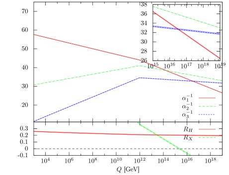
(a) $M_{\lambda}=m_{0}=m_{\Sigma}=m_{H_{C}}=10^{12}~{}{\rm GeV}$

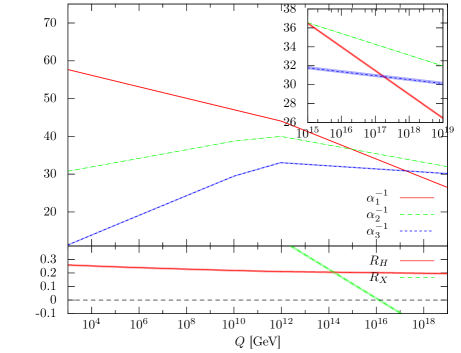
(b) $10^{2}M_{\lambda}=m_{0}=m_{\Sigma}=m_{H_{C}}=10^{12}~{}{\rm GeV}$

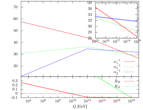
(c) Same as (a) except that $M_{\tilde{W}}=1~{}{\rm TeV}$

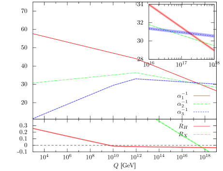
(d) Same as (b) except that $M_{\tilde{W}}=1~{}{\rm TeV}$

Figure 3: The renormalization group running of the SM gauge couplings for representative spectra in the ISS model. Each shaded band represents the 3-$\sigma$ experimental uncertainty for the gauge coupling. Here, we have assumed $\tan\beta=1$. Important combinations of the gauge couplings, $R_{X}$ and $R_{H}$ defined in Eqs. (23, 24), are also plotted; they determine the scale and precision of unification, as in Eqs. (26, 27).

In Fig. 3, we show the running of the SM gauge couplings for some selected ISS mass spectra. In Fig. 3(a) we show the case in which all the superpartners and (uneaten) GUT particles have a common mass of $\tilde{m}=10^{12}~{}{\rm GeV}$ (corresponding to the case with $m_{\rm LSP}\sim O(\tilde{m})$ in the previous subsection, while in Fig. 3(b) we set the gaugino masses $M_{\lambda}$ to be suppressed by a factor of $100$ compared with the rest of the intermediate scale particles. We find that the unification scale, determined by Eq. (26), is

$$M_{X}\sim 10^{16}~{}{\rm GeV}\quad\mbox{for}\quad m_{\rm LSP}\sim O(\tilde{m}).$$ (28)

The size of the threshold correction, determined by Eq. (27) with $M_{H_{C}}\sim O(\tilde{m})$, is $|aV/\Lambda|\approx 0.2$. In Figs. 3(c) and 3(d), we show the same plots as Figs. 3(a) and 3(b), respectively, except that the wino mass is lowered to $1~{}{\rm TeV}$. This slightly raises the unification scale

$$M_{X}\sim 10^{17}~{}{\rm GeV}\quad\mbox{for}\quad m_{\tilde{W}}\sim{\rm TeV},$$ (29)

and improves the precision for gauge coupling unification; the required size of the threshold correction from the dimension-five operator is now $|aV/\Lambda|\lesssim 0.1$.

We finally comment on bottom-tau Yukawa unification. In the minimal ISS model discussed here, the ratio of the two couplings is $y_{b}/y_{\tau}\simeq 0.6$ at the GUT scale, so that it requires a relatively large threshold correction to be compatible with the GUT embedding of the quarks and leptons. This can be achieved, for example, by taking $(y_{D})_{33}\lesssim(\eta_{D})_{33}$ in Eq. (15). Similar GUT-violating contributions may also be needed to accommodate the observed quark and lepton masses for lighter generations.

3.4 Proton decay

Here we discuss proton decay. As we have seen, the mass of the $XY$ GUT gauge bosons, $M_{X}$, is comparable or larger than in the conventional weak-scale SSM. In particular, when the wino is at a TeV, $M_{X}\sim 10^{17}~{}{\rm GeV}$ as in Eq. (29), so that dimension-six proton decay caused by gauge boson exchange is suppressed.

How about proton decay caused by exchange of colored Higgs fields, which now have masses of order $\tilde{m}\ll\langle\Sigma\rangle$? In the conventional weak-scale SSM, the colored Higgs supermultiplets $H_{C}$ and $\bar{H}_{C}$ induce large proton decay rates. In this case the dominant contributions come from one-loop diagrams involving weak-scale superpartners with amplitudes suppressed only by $1/(M_{H_{C}}m_{\rm soft})$, where $m_{\rm soft}\sim v$ is the mass of the weak-scale superpartners. To avoid rapid proton decay, we need to push the mass of the colored Higgs multiplets to be very large [33]. If the sfermion mass scale is much larger than the weak scale, however, the proton decay rate from these processes (dimension-five proton decay) can be suppressed, and the constraints can accordingly be relaxed [34].

In ISS models, the sfermion mass scale is quite large, $\tilde{m}\gg v$, so that dimension-five proton decay can be suppressed, which allows us to take $M_{H_{C}}\sim O(\tilde{m})$ as has been described so far. In fact, unlike the conventional case, the dominant contribution to proton decay typically comes from tree-level colored Higgs-boson exchange, as shown in Fig. 4(a). This contribution is suppressed by $1/M_{H_{C}}^{2}$ in the amplitude, and is negligible in conventional GUTs; but here the suppression is only $1/M_{H_{C}}^{2}\sim O(1/\tilde{m}^{2})$, and its amplitude is larger than that for dimension-five proton decay by a one-loop factor. The dominant decay mode is expected to be $p\rightarrow\bar{\nu}K^{+}$, with lifetime given approximately by

$$\tau_{p}\approx O(10^{32}\mbox{--}10^{33})\left(\frac{M_{H_{C}}}{10^{11}~{}{\rm GeV}}\right)^{4}~{}{\rm years}.$$ (30)

The current limit from the Super-Kamiokande experiment is $\tau_{p}(p\rightarrow\bar{\nu}K^{+})>5.9\times 10^{33}~{}{\rm years}$ at 90% confidence level [35], so that $M_{H_{C}}$ greater than $O(10^{11}~{}{\rm GeV})$ is consistent with the latest observation. This limit is expected to be improved to $2.5\times 10^{34}~{}{\rm year}$ in the hyper-Kamiokande experiment [36].

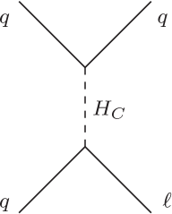
(a) Tree level

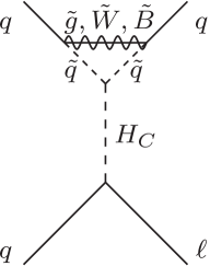
(b) One-loop level

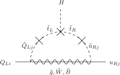
(c) Correction to Yukawa couplings

Figure 4: Examples of diagrams relevant for proton decay.

The proton decay rate in Eq. (30) is subject to several uncertainties. One of them comes from GUT $CP$ phases; there are two additional physical $CP$ phases in the colored Higgs Yukawa couplings, which cannot be determined by the SSM Yukawa couplings. Depending on these phases, cancellation between Wilson operators causing the proton decay may occur. This leads to an $O(10)$ uncertainty in the estimate of the proton lifetime. (We will see this uncertainty explicitly in the study of the mSUGRA example in the next subsection.) Another source of uncertainties comes from the long distance QCD contribution to the proton decay matrix elements, which also leads to an $O(10)$ uncertainty in the lifetime estimate. Furthermore, as we discussed before, accommodating the observed quark and lepton masses in the model requires contributions from higher-dimensional operators to the Yukawa couplings. These operators also affect the estimate of the proton decay rate.

We finally comment on contributions from loop diagrams. As discussed in Ref. [37], if the sfermion sector has large flavor violation, loop contributions may be significantly enhanced. For instance, large flavor violation in the squark masses can induce large corrections to the first and second generation Yukawa couplings, as in Fig. 4(c), and accordingly large corrections to the colored Higgs Yukawa couplings. In some cases, proton decay induced through such one-loop diagrams may dominate over the tree-level contribution. The importance of one-loop processes, however, depends strongly on the gaugino masses, the structure of sfermion flavor violation, GUT-violating threshold corrections from higher dimension operators, and so on. For example, amplitudes of Figs. 4(b) and 4(c) are proportional to the gaugino masses, so that smaller gaugino masses result in smaller contributions. Also, flavor violation in ${\bf 5}^{*}$ matter, $\bar{F}(d,l)$, generically leads to smaller effects on proton decay than that in ${\bf 10}$ matter, $T(q,u,e)$, and, depending on the size of the GUT-violating effects, cancellations between contributions from Figs. 4(b) and 4(c) may occur. The general study of all these effects is thus highly complicated. In the explicit analysis in the next subsection, we ignore these possible corrections and assume, for simplicity, minimal flavor violation for the relevant flavor structure.

3.5 Example: mSUGRA-like spectrum

In this subsection, we present a detailed study of the model described here in the case that the supersymmetry breaking masses obey mSUGRA-like boundary conditions. Specifically, we set the following boundary conditions for the relevant parameters at the renormalization scale $Q_{0}=10^{17}~{}{\rm GeV}$:

$$m^{2}_{T({\bf 10})}=m^{2}_{\bar{F}({\bf 5}^{*})}=\tilde{m}^{2}\,{\bf 1}_{3\times 3},\qquad m^{2}_{H_{u}}=m^{2}_{H_{d}}=m^{2}_{H_{C}}=m^{2}_{\bar{H}_{C}}=\tilde{m}^{2},$$ (31)

$$M_{\tilde{B}}=M_{\tilde{W}}=M_{\tilde{g}}=m_{1/2},\qquad\mu=\mu_{H_{C}},\qquad B=B_{H_{C}}.$$ (32)

The $A$ terms are set to zero, and the mass of the uneaten components of $\Sigma$ is taken to be $\tilde{m}$. Here, we have ignored possible GUT breaking effects for the above parameters. While the running mass of the wino obtained from these boundary conditions is typically large, we assume that its physical mass is $1~{}{\rm TeV}$ as a result of cancellations among various, including threshold, contributions. (This assumption affects renormalization group evolution from TeV to $\tilde{m}$.) We set the Yukawa interactions between the colored Higgs and matter fields by matching them with the SSM Yukawa couplings $y_{u}$ and $y_{d}$; see Ref. [37] for details. In the analysis below, we treat $\tan\beta$ as an input parameter, trading $\mu$ and $B$ with $v$ and $\tan\beta$ by the electroweak symmetry breaking condition, as in conventional mSUGRA analyses.

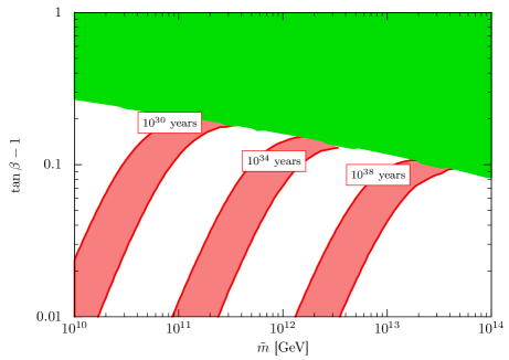
(a) $\tau_{p}(p\rightarrow\bar{\nu}K^{+})$

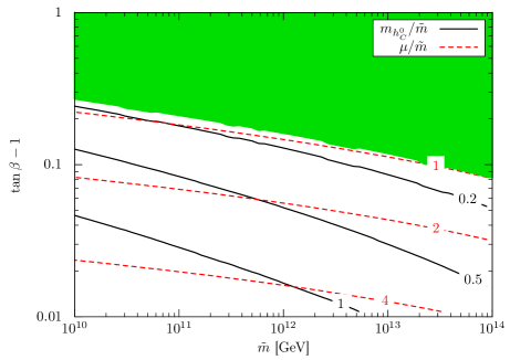
(b) Masses in the Higgs sector

Figure 5: (a) Proton lifetime for the $\bar{\nu}K^{+}$ mode and (b) $m_{h^{0}_{C}}/\tilde{m}$ (black solid) and $\mu/\tilde{m}$ (red dashed) for the mSUGRA-like boundary conditions in Eqs. (31, 32) with $m_{1/2}=0.01\tilde{m}$. The boundary conditions in Eq. (31) exclude the green regions at the top. The red bands for the proton lifetime represent uncertainties from the GUT $CP$ phases discussed in Section 3.4.

In Fig. 5, we show the proton lifetime of $p\rightarrow\bar{\nu}K^{+}$ (in 5(a)) and the masses of the lightest colored Higgs scalar ${h^{0}_{C}}$ and $\mu$ (in 5(b)) in the $\tilde{m}$-$\tan\beta$ plane. Here, we have set $m_{1/2}/{\tilde{m}}=0.01$. The green shaded region in the upper region of each plot represents parameter space in which correct electroweak symmetry breaking cannot occur. We find that $\tan\beta-1$ cannot be larger than $O(0.1)$. This is because the boundary condition $m_{H_{u}}^{2}=m_{H_{d}}^{2}$ at $Q=Q_{0}$ implies $m_{H_{u}}^{2}\approx m_{H_{d}}^{2}$ at $Q=\tilde{m}$, leading to $\tan\beta\approx 1$; see Eq. (13). (The electroweak symmetry can be broken by $B$.) Because $\tan\beta\sim 1$, essentially all the allowed region with $\tilde{m}\approx O(10^{9}\mbox{--}10^{13}~{}{\rm GeV})$ and $\mu/\tilde{m}\lesssim 4$ is consistent with the observed Higgs boson mass, $m_{h^{0}}\simeq 125~{}{\rm GeV}$. (For $\mu\gg\tilde{m}$, there could be significant threshold corrections to $\lambda$, making it deviate from the condition $\lambda(\tilde{m})\approx 0$.) The red bands in Fig. 5(a) represent uncertainties from the GUT $CP$ phases discussed in Section 3.4. In calculating the proton decay rate, we have used the CKM matrix in Ref. [38], the PDG average of the light quark masses [39], and the four-loop renormalization group equations and three-loop decoupling effects from heavy quarks [40] to estimate the Yukawa couplings of the light quarks. We have followed Ref. [41] to obtain the Wilson operators relevant for the proton decay at the hadronic scale, and used matrix elements in Ref. [42].

In Fig. 5(b), we see that $\mu/\tilde{m}$ increases as we go lower in the plot. This is because the value of $\tan\beta$ is given by

$$\tan\beta-1\approx\frac{m_{H_{d}}^{2}-m_{H_{u}}^{2}}{2|\mu|^{2}}\Biggr{|}_{Q\approx\tilde{m}}\approx O\biggl{(}\frac{\tilde{m}^{2}}{|\mu|^{2}}\biggr{)},$$ (33)

for $|\mu|^{2}\gtrsim\tilde{m}^{2}$. Note that we need not have an extreme fine-tuning between $m_{H_{u}}^{2}$ and $m_{H_{d}}^{2}$ to obtain $\tan\beta\ll 1$ for $|\mu|$ reasonably larger than $\tilde{m}$. In the figure, we also find that the lightest colored Higgs scalar ${h^{0}_{C}}$ is a factor of a few lighter than the heavier (colored and non-colored) Higgs bosons, whose masses are around $|\mu|\sim|\mu_{H_{C}}|$. This is because $h^{0}_{C}$ is almost the GUT partner of the light fine-tuned SM Higgs $h^{0}$, so that its mass is suppressed due to the approximate GUT relation between the color-triplet and weak-doublet Higgs mass-squared matrices, which is broken here only by the renormalization group running effect between $Q_{0}$ and $\tilde{m}$. Note that the dominant contribution to proton decay comes from exchange of $h^{0}_{C}$, with the rate proportional to the inverse fourth powers in the mass of $h^{0}_{C}$. This implies that the proton decay rate is highly sensitive to possible GUT-violating threshold corrections at $Q_{0}$. For example, an $O(10\%)$ violating of, e.g., the relation $\mu=\mu_{H_{C}}$ or $m^{2}_{H_{u},H_{d}}=m^{2}_{H_{C},\bar{H}_{C}}$ could lead to a change of the proton decay rate by a couple of orders of magnitude.

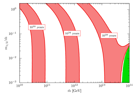
(a) $\tau_{p}(p\rightarrow\bar{\nu}K^{+})$

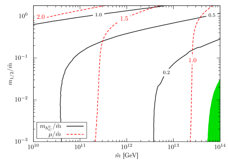
(b) Masses in the Higgs sector

Figure 6: Same quantities as in Fig. 5 plotted in the $\tilde{m}$-$m_{1/2}/\tilde{m}$ plane. We have set $\tan\beta=1.1$.

In Fig. 6, we show the same quantities as in Fig. 5 in the $\tilde{m}$-$m_{1/2}/\tilde{m}$ plane by taking $\tan\beta=1.1$. As we increase $m_{1/2}/\tilde{m}$, the mass of $h^{0}_{C}$ becomes larger and, accordingly, the lifetime of the proton for fixed $\tilde{m}$ increases. This is because larger $m_{1/2}/\tilde{m}$ leads to a larger violation of the GUT relation between the mass-squared matrices for the color-triplet and weak-doublet Higgses, so that electroweak fine-tuning for the mass of $h^{0}$ yields less suppression for the mass of $h^{0}_{C}$.

4 ISS as the Origin of Scales for New Physics

In this section, we argue that the mass scale $\tilde{m}$ in ISS may provide the origin of a variety of new physics occurring at intermediate scales, Eq. (2). Specifically, we consider the heavy mass scale for seesaw neutrino masses, the axion decay constant, and the inflaton mass as originating from $\tilde{m}$. The discussions here are not contingent on the specific model presented in the previous section or in Ref. [4], and apply more generally to a large classes of ISS models. Also, all the mechanisms described below need not be realized simultaneously; one or more of the mass scales appearing in these phenomena may originate from other physics.

4.1 Seesaw neutrino masses

The simplest understanding of small neutrino masses follows from having lepton number broken at a very high scale, $M_{L}$. At energies below $M_{L}$, lepton number becomes an accidental symmetry of interactions up to dimension 4, yielding Majorana neutrino masses at dimension 5 via $ll\,hh/M_{L}$. Within ISS it is natural to associate $M_{L}$ with $\tilde{m}$, since this is the only mass scale below the cutoff, giving neutrino masses of $m_{\nu}\sim v^{2}/\tilde{m}$.

We can implement this by introducing $SU(5)$ singlet right-handed neutrino superfields, $N$, neutral under $U(1)_{R}$, so that the Kähler potential contains $c_{\nu}NN/2$, with $c_{\nu}$ being $O(1)$ coefficients. Once supersymmetry is broken, the supergravity interactions generate an effective superpotential $W_{\rm eff}^{\nu}=\tilde{m}_{\nu}NN/2$, where $\tilde{m}_{\nu}$ is a $3\times 3$ matrix in flavor space with entries order $\tilde{m}$. Introducing a $3\times 3$ Yukawa coupling matrix $y_{\nu}$ via the superpotential interaction $y_{\nu}N\bar{F}H$ leads to a light neutrino mass matrix

$$m_{\nu}=\left(y_{\nu}^{T}\,\frac{1}{\tilde{m}_{\nu}}\,y_{\nu}\right)v^{2}.$$ (34)

For example, with $\tilde{m}=10^{13}~{}{\rm GeV}$, the observed neutrino masses result from $y_{\nu}$ entries of order $0.1$.

Previously we have used a $U(1)_{R}$ symmetry with charges $R=0$ for $H,\bar{H},\Sigma$ and $R=1$ for $T,\bar{F}$. This symmetry does not work in the present case, since the $y_{\nu}N\bar{F}H$ couplings would then imply $N$’s having $R=1$, so that $K\supset c_{\nu}NN/2$ cannot be written while the $N^{2}$ terms are allowed in the superpotential. Assuming that the supersymmetry breaking field $X$ is neutral under it, we find a unique flavor-independent $R$ symmetry that allows both $c_{\nu}$ and $y_{\nu}$ to be non-zero: $R^{\prime}=R-X/5$, where $U(1)_{X}$ is the Abelian generator that appears in $SO(10)/SU(5)$ and has charges $T(1),\bar{F}(-3),N(5),H(-2),\bar{H}(2),\Sigma(0)$, and we have chosen $R=1$ for $N$. Imposing this $U(1)_{R^{\prime}}$ symmetry yields a theory with the general structure

$$\tilde{K} =\Lambda^{2}\,f\Bigl{(}\frac{\Sigma}{\Lambda},\frac{H\bar{H}}{\Lambda^{2}},\frac{NN}{\Lambda^{2}}\Bigr{)},$$ (35)

$$W =y_{U}\Bigl{(}\frac{\Sigma}{\Lambda}\Bigr{)}\,TTH+y_{D}\Bigl{(}\frac{\Sigma}{\Lambda}\Bigr{)}\,T\bar{F}\bar{H}+y_{\nu}\Bigl{(}\frac{\Sigma}{\Lambda}\Bigr{)}\,N\bar{F}H,$$ (36)

leading to the neutrino mass matrix in Eq. (34). Here, $\tilde{K}$ is the holomorphic part of the Kähler potential, and we have imposed matter parity under which $\Sigma,H,\bar{H}$ are even while $T,\bar{F},N$ are odd.

It is interesting to note that values of the right-handed neutrino masses implied by the above mechanism are consistent with thermal leptogenesis, which works for a wide range of conditions after inflation if the lightest right-handed neutrino is heavier than about $10^{9}~{}{\rm GeV}$ for hierarchical right-handed neutrinos [43].

4.2 Axion

One of the major problems in the SM is the strong $CP$ problem. A promising solution is to introduce an anomalous Peccei-Quinn (PQ) symmetry spontaneously broken at a scale $f_{a}$, leading to an axion field with decay constant $f_{a}$. Here we consider that the scale of $f_{a}$ is given by $\tilde{m}$, and present a simple model realizing this idea. For a different implementation of a similar setup, in which $f_{a}$ is related to $\tilde{m}$, see Ref. [44].

We consider the superpotential of the form

$$W\supset c\,SQ\bar{Q}+c^{\prime}\,S^{2}\bar{S}.$$ (37)

Here, $c$ and $c^{\prime}$ are coefficients of order unity, and chiral superfields $S$ (which will be identified as the PQ-breaking field), $\bar{S},Q$, and $\bar{Q}$ have the $U(1)$ PQ charges

$$S(1),\quad\bar{S}(-2),\quad Q\bar{Q}(-1).$$ (38)

The superpotential of the above form may be used to build a variety of axion models, including DFSZ-type models in which a part of $Q$ and $\bar{Q}$ may be identified with the SSM Higgs doublets. Here we choose the following simple $SU(5)$ representation

$$S({\bf 1}),\quad\bar{S}({\bf 1}),\quad Q({\bf 5}),\quad\bar{Q}({\bf 5}^{*}).$$ (39)

Since $Q$ and $\bar{Q}$ comprise complete $SU(5)$ multiplets, gauge coupling unification is preserved. This simple choice also guarantees that the so-called domain wall number $N_{\rm DW}$ is unity, which allows us to avoid stringent cosmological constraints as discussed below.

Once supersymmetry is broken, the $S$ field may have a negative soft supersymmetry-breaking mass-squared of order $\tilde{m}^{2}$:

$$V\supset-m_{S}^{2}S^{\dagger}S,\qquad m_{S}^{2}\sim O(\tilde{m}^{2}).$$ (40)

Indeed, this negative mass-squared may be induced radiatively through renormalization group running from $M_{*}$ ($\sim\Lambda\sim M_{\rm Pl}$) to the scale $\tilde{m}$, starting from the boundary condition that all the fields have positive soft squared masses at $M_{*}$, in which case the soft supersymmetry-breaking squared masses for $\bar{S}$, $Q$, and $\bar{Q}$ will be positive. The potential given by Eqs. (37, 40) leads to a vacuum at

$$\langle S\rangle=f_{a}\sim O(\tilde{m}),\qquad\langle\bar{S}\rangle=\langle Q\rangle=\langle\bar{Q}\rangle=0,$$ (41)

breaking the PQ symmetry at $\sim\tilde{m}$. As a result, all the particles in the $S,\bar{S},Q,\bar{Q}$ multiplets receive masses of order $\tilde{m}$ except for the light Nambu-Goldstone axion field arising from $S$, whose decay constant is given by $\langle S\rangle=f_{a}$.

The recent discovery of the $B$-mode polarization in cosmic microwave background radiation by BICEP2 collaboration [16], $r=0.2^{+0.07}_{-0.05}$, suggests that the scale of inflation is large:

$$H_{I}\simeq 7.8\times 10^{13}~{}{\rm GeV}\left(\frac{r}{0.1}\right)^{1/2},$$ (42)

where $H_{I}$ is the Hubble parameter during inflation. This has significant impacts on axion models. If the PQ symmetry is broken before inflation, the light axion field produces isocurvature perturbation. With the large inflation scale in Eq. (42), this case is excluded by observation [45], unless the dynamics associated with the PQ symmetry breaking is somewhat complicated, e.g., if $f_{a}$ is much larger [46] or if the axion is heavier than $H_{I}$ [47] during inflation due to nontrivial dynamics.

We thus consider here the case in which the PQ symmetry is broken after the end of inflation. In this case, topological objects formed associated with PQ symmetry breaking, in particular domain walls, may give serious cosmological problems [48]. In the model presented above, however, the domain wall number is unity, $N_{\rm DW}=1$, so that domain walls, which are disk-like objects bounded by strings, are unstable [49]. The decay of these domain walls produces axion particles, but a detailed lattice simulation indicates that the value of $f_{a}\lesssim\mbox{a few}\times 10^{10}~{}{\rm GeV}$ is consistent with the current observation [50]. (A slightly weaker estimate of $f_{a}\lesssim 10^{11}~{}{\rm GeV}$, coming from the misalignment mechanism of dark matter production, is implied by the analysis in Ref. [51].) Together with the lower bound on $f_{a}$ from stellar physics (for reviews on axion physics, see e.g. [52]), we find that

$$f_{a}\approx O(10^{9}\mbox{--}10^{11}~{}{\rm GeV}),$$ (43)

gives consistent phenomenology. (We expect that the axino and saxion do not cause cosmological problems in the present model, since they are heavy with masses of order $\tilde{m}$. The $Q$ and $\bar{Q}$ states may also be made to decay by coupling them with SM particles, without violating the PQ symmetry.) The value of $f_{a}$ in Eq. (43) can be easily obtained with $\tilde{m}$ in the ISS range, suggested by the observed Higgs boson mass.

4.3 Inflation

A very simple inflation model is given by the following potential for the inflaton $\phi$:

$$V(\phi)=\frac{m_{\phi}^{2}}{2}\,\phi^{2}.$$ (44)

Interestingly, this simple potential gives a good agreement with the observations of the scalar spectral index $n_{s}$ by Planck [53] and the tensor-to-scalar ration $r$ by BICEP2 [16] for

$$m_{\phi}\simeq 10^{13}~{}{\rm GeV}.$$ (45)

It is, therefore, interesting to identify $m_{\phi}$ as $\tilde{m}$, which is roughly in the same energy range.

The construction of a complete inflation model in supergravity realizing the above idea, however, is challenging, since the value of field $\phi$ during inflation is beyond the reduced Planck scale $M_{\rm Pl}$, where the scalar potential obtained from supergravity loses theoretical control. Moreover, depending on the mechanism of how the supersymmetry breaking masses are generated, the soft supersymmetry breaking mass for $\phi$ may be shut off above some scale, e.g., $M_{*}$. One possibility is to use a shift symmetry on $\phi$ along the lines of, e.g., Ref. [55], but the construction of an explicit model seems nontrivial. Another possibility is that the apparent obstruction in supergravity of having flat potential beyond $\phi\approx M_{\rm Pl}$ is not warranted, as has been discussed, e.g., in Ref. [56] and more recently in Ref. [57].

An alternative direction for realizing the idea of connecting the ISS scale with inflation is to use the constant term in the superpotential, $W_{0}$, needed to cancel the cosmological constant. If we assume that the superpartner mass scale $\tilde{m}$ is generated by some mediation mechanism at $M_{*}$, the $F$-term VEV for the supersymmetry breaking field is given by $F\sim\tilde{m}M_{*}$. This implies that $W_{0}\sim\tilde{m}M_{*}M_{\rm Pl}$. Taking $M_{*}\sim M_{\rm Pl}$, this scale is thus

$$W_{0}^{1/3}\sim 10^{16}\left(\frac{\tilde{m}}{10^{12}~{}{\rm GeV}}\right)^{1/3}{\rm GeV},$$ (46)

which is very close to the energy scale during inflation $V_{I}^{1/4}\simeq 2\times 10^{16}~{}{\rm GeV}$ suggested by the BICEP2 data. Inflation, therefore, may occur associated with the dynamics generating this constant term, for example through some gaugino condensations, along the lines of, e.g., Ref. [58]. We leave explorations of explicit inflation models in the ISS framework to future work.

5 Summary

We have explored supersymmetric grand unified theories that have a single scale, that of supersymmetry breaking, determined by the value of the Higgs boson mass to be in the intermediate range of $\tilde{m}\sim 10^{9}\mbox{--}10^{13}~{}{\rm GeV}$. Mass terms for the $SU(5)$ Higgs multiplets, $\Sigma,H,\bar{H}$ are generated at $\tilde{m}$ in the same way that in minimal supersymmetric models the Higgs mass parameter $\mu$ can arise at the supersymmetry breaking scale. However, unlike electroweak breaking in these minimal models, the breaking of the unified symmetry by $\Sigma$ occurs at a scale parametrically higher than $\tilde{m}$, close to the cutoff scale of the theory.

A variety of diverse physics can be described by such GUTs with ISS, as illustrated in Fig. 7. For a wide range of parameters, the SM Higgs quartic coupling is constrained to be small at $\tilde{m}$; indeed we determine the allowed range of $\tilde{m}$ by using the Higgs mass as input as shown in Fig. 1. The result is illustrated by the upper horizontal green bar in Fig. 7, showing the range of the scale $\mu_{c}$ where the quartic coupling vanishes in the SM (possibly augmented by a TeV wino for dark matter).

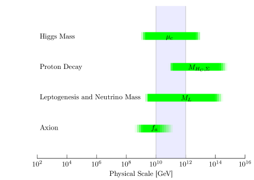
Figure 7: The experimentally allowed ranges of four key mass scales: $\mu_{c}$ (the scale at which the SM Higgs quartic coupling vanishes); $M_{H_{C},\Sigma}$ (the masses of the $H_{c}$ and $\Sigma$ states in the ISS model of Section 3); $M_{L}$ (the scale of lepton number violation for seesaw neutrino masses and leptogenesis); and $f_{a}$ (the axion decay constant in minimal models that solve the strong $CP$ problem). All are consistent with ISS, with supersymmetry breaking centered around the shaded region.

In the minimal ISS model, introduced and studied in depth in Section 3, proton decay is induced by both the tree-level exchange of the colored triplet $SU(5)$ partner of the Higgs boson $H_{C}$, of mass $M_{H_{C}}$, and by the exchange of the GUT gauge bosons $X$. The mass of $H_{C}$ is expected to be comparable to the mass of the uneaten states in $\Sigma$, $M_{\Sigma}$, and the experimental constraint on these masses is shown in the second horizontal green bar of Fig. 7. The lower end of the range results from the limit on $p\rightarrow\bar{\nu}K^{+}$ from $H_{C}$ exchange, while the upper end of the range arises from the limit on $p\rightarrow e^{+}\pi^{0}$ from $X$ exchange; the mass of $X$ being sensitive to $M_{\Sigma}$ via gauge coupling unification. Even though there are order unity couplings that lead to differences between $\mu_{c}$ and $M_{H_{C},\Sigma}$, it is important for the consistency of the theory that the ranges of the top two green bars overlap. While the presence of $\Sigma$ states at $\tilde{m}$ solves the proton decay problem of non-supersymmetric $SU(5)$, having $H_{C}$ states at $\tilde{m}$ does not introduce a new proton decay problem, but offers the possibility of a signal. The precision of gauge coupling unification is further enhanced if dark matter is environmentally selected by fine-tuning the wino mass to the TeV region.

The basic model of Section 3 leaves open two key questions, the origin of neutrino masses and inflation. Seesaw neutrino masses occur very naturally in our framework as the lepton number violating mass for the right-handed neutrinos, $M_{L}$, can arise from the same mechanism that generates the masses for $\Sigma,H,\bar{H}$. The experimentally allowed range for $M_{L}$ is shown by the third horizontal bar in Fig. 7. The upper end of the range arises from the need to explain the size of the atmospheric neutrino oscillation, and is shown for neutrino Yukawa couplings of order unity, while the lower end arises from the requirement of a leptogenesis origin for the cosmological baryon asymmetry. Note that leptogenesis also requires that $M_{L}$ be less than the reheat temperature after inflation, so that the upper bound on $M_{L}$ may be lower than shown.

Recent data from BICEP2 indicates that the scale of the vacuum energy that drives inflation is $\simeq 2\times 10^{16}~{}{\rm GeV}$. However, this need not be a Lagrangian mass scale; for example, for an inflation potential $m_{\phi}^{2}\phi^{2}/2$ the required inflaton mass is $m_{\phi}\simeq 10^{13}~{}{\rm GeV}$. We do not show this in Fig. 7 because it is specific to this particular potential. However, it is certainly consistent with the masses $\mu_{c},M_{H_{c},\Sigma},M_{L}$, so we may expect that this also arises from $\tilde{m}$.

Finally, the axion is the most promising solution to the strong $CP$ problem, and may also account for dark matter. The large value of the Hubble parameter during inflation indicated by the BICEP2 data, implies that the simplest axion models having PQ symmetry broken during inflation are excluded. In Fig. 7 we therefore show the experimentally allowed range of the axion decay constant in theories having a PQ phase transition after inflation. The upper limit arises from overclosure by axions, and the lower limit from axion emission from supernovae and white dwarfs. Again, from Fig. 7 we notice a remarkable consistency between the mass scales required for very different physics; in ISS these masses are not precisely equal, but may all arise from $\tilde{m}$, the scale of supersymmetry breaking.

References

- [1] L. J. Hall and Y. Nomura, JHEP 03, 076 (2010) [arXiv:0910.2235 [hep-ph]].
- [2] A. Hebecker, A. K. Knochel and T. Weigand, JHEP 06, 093 (2012) [arXiv:1204.2551 [hep-th]]; Nucl. Phys. B 874, 1 (2013) [arXiv:1304.2767 [hep-th]].
- [3] L. E. Ibáñez, F. Marchesano, D. Regalado and I. Valenzuela, JHEP 07, 195 (2012) [arXiv:1206.2655 [hep-ph]]; L. E. Ibáñez and I. Valenzuela, JHEP 05, 064 (2013) [arXiv:1301.5167 [hep-ph]].
- [4] L. J. Hall and Y. Nomura, JHEP 02, 129 (2014) [arXiv:1312.6695 [hep-ph]].
- [5] S. Weinberg, Phys. Rev. Lett. 59, 2607 (1987); see also, T. Banks, Nucl. Phys. B 249, 332 (1985); A. D. Linde, Rept. Prog. Phys. 47, 925 (1984).
- [6] V. Agrawal, S. M. Barr, J. F. Donoghue and D. Seckel, Phys. Rev. D 57, 5480 (1998) [arXiv:hep-ph/9707380]; T. Damour and J. F. Donoghue, Phys. Rev. D 78, 014014 (2008) [arXiv:0712.2968 [hep-ph]].
- [7] The ATLAS, CDF, CMS and D0 Collaborations, arXiv:1403.4427 [hep-ex].
- [8] The ATLAS Collaboration, ATLAS-CONF-2013-014.
- [9] S. Chatrchyan et al. [CMS Collaboration], JHEP 06, 081 (2013) [arXiv:1303.4571 [hep-ex]].
- [10] M. Baak and R. Kogler, arXiv:1306.0571 [hep-ph].
- [11] S. Bethke, Nucl. Phys. Proc. Suppl. 234, 229 (2013) [arXiv:1210.0325 [hep-ex]].
- [12] G. F. Giudice and A. Strumia, Nucl. Phys. B 858, 63 (2012) [arXiv:1108.6077 [hep-ph]]; D. Buttazzo, G. Degrassi, P. P. Giardino, G. F. Giudice, F. Sala, A. Salvio and A. Strumia, JHEP 12, 089 (2013) [arXiv:1307.3536]; see also A. Delgado, M. Garcia and M. Quiros, arXiv:1312.3235 [hep-ph].
- [13] G. Elor, H.-S. Goh, L. J. Hall, P. Kumar and Y. Nomura, Phys. Rev. D 81, 095003 (2010) [arXiv:0912.3942 [hep-ph]].
- [14] L. Hall, J. D. Lykken and S. Weinberg, Phys. Rev. D 27, 2359 (1983).
- [15] W. Siegel and S. J. Gates Jr., Nucl. Phys. B 147, 77 (1979).
- [16] P. A. R. Ade et al. [BICEP2 Collaboration], arXiv:1403.3985 [astro-ph.CO].
- [17] L. Randall and R. Sundrum, Nucl. Phys. B 557, 79 (1999) [hep-th/9810155]; G. F. Giudice, M. A. Luty, H. Murayama and R. Rattazzi, JHEP 12, 027 (1998) [hep-ph/9810442].
- [18] L. J. Hall and Y. Nomura, JHEP 01, 082 (2012) [arXiv:1111.4519 [hep-ph]].
- [19] F. Takayama, Phys. Rev. D 77, 116003 (2008) [arXiv:0704.2785 [hep-ph]].
- [20] M. Tegmark, A. Aguirre, M. J. Rees and F. Wilczek, Phys. Rev. D 73, 023505 (2006) [astro-ph/0511774]; R. Bousso and L. Hall, Phys. Rev. D 88, 063503 (2013) [arXiv:1304.6407 [hep-th]].
- [21] J. Hisano, S. Matsumoto, M. Nagai, O. Saito and M. Senami, Phys. Lett. B 646, 34 (2007) [hep-ph/0610249].
- [22] J. L. Feng, T. Moroi, L. Randall, M. Strassler and S. Su, Phys. Rev. Lett. 83, 1731 (1999) [hep-ph/9904250]; M. Ibe, S. Matsumoto and R. Sato, Phys. Lett. B 721, 252 (2013) [arXiv:1212.5989 [hep-ph]].
- [23] M. Ibe, T. Moroi and T. T. Yanagida, Phys. Lett. B 644, 355 (2007) [hep-ph/0610277]; M. R. Buckley, L. Randall and B. Shuve, JHEP 05, 097 (2011) [arXiv:0909.4549 [hep-ph]].
- [24] S. Asai, T. Moroi, K. Nishihara and T. T. Yanagida, Phys. Lett. B 653, 81 (2007) [arXiv:0705.3086 [hep-ph]]; S. Asai, T. Moroi and T. T. Yanagida, Phys. Lett. B 664, 185 (2008) [arXiv:0802.3725 [hep-ph]]; S. Asai, Y. Azuma, O. Jinnouchi, T. Moroi, S. Shirai and T. T. Yanagida, Phys. Lett. B 672, 339 (2009) [arXiv:0807.4987 [hep-ph]].
- [25] The ATLAS Collaboration, Phys. Rev. D 88, 112006 (2013) [arXiv:1310.3675 [hep-ex]].
- [26] K. Ichikawa, talk presented at the 30th General Meeting of the ILC Physics Subgroup, Mar. 16 (2013), KEK, Japan: http://ilcphys.kek.jp/meeting/physics/archives/2013-03-16
- [27] J. Hisano, S. .Matsumoto, M. M. Nojiri and O. Saito, Phys. Rev. D 71, 063528 (2005) [hep-ph/0412403].
- [28] J. Hisano, S. Matsumoto, O. Saito and M. Senami, Phys. Rev. D 73, 055004 (2006) [hep-ph/0511118];
- [29] T. Cohen, M. Lisanti, A. Pierce and T. R. Slatyer, JCAP 10, 061 (2013) [arXiv:1307.4082]; J. Fan and M. Reece, JHEP 10, 124 (2013) [arXiv:1307.4400 [hep-ph]].
- [30] A. Hryczuk, I. Cholis, R. Iengo, M. Tavakoli and P. Ullio, arXiv:1401.6212 [astro-ph.HE].
- [31] M. Pato, D. Hooper and M. Simet, JCAP 06, 022 (2010) [arXiv:1002.3341 [astro-ph.HE]].
- [32] L. J. Hall, Y. Nomura and S. Shirai, JHEP 01, 036 (2013) [arXiv:1210.2395 [hep-ph]].
- [33] See, e.g., H. Murayama and A. Pierce, Phys. Rev. D 65, 055009 (2002) [hep-ph/0108104].
- [34] J. Hisano, D. Kobayashi, T. Kuwahara and N. Nagata, JHEP 07, 038 (2013) [arXiv:1304.3651 [hep-ph]].
- [35] E. Kearns, talk presented at ISOUP 2013, May 24-27 (2013), Asilomar, California.
- [36] K. Abe et al., arXiv:1109.3262 [hep-ex].
- [37] N. Nagata and S. Shirai, JHEP 03, 049 (2014) [arXiv:1312.7854 [hep-ph]].
- [38] UTfit, http://www.utfit.org/UTfit/WebHome
- [39] J. Beringer et al. [Particle Data Group Collaboration], Phys. Rev. D 86, 010001 (2012).
- [40] K. G. Chetyrkin, B. A. Kniehl and M. Steinhauser, Phys. Rev. Lett. 79, 2184 (1997) [hep-ph/9706430].
- [41] L. F. Abbott and M. B. Wise, Phys. Rev. D 22, 2208 (1980); T. Nihei and J. Arafune, Prog. Theor. Phys. 93, 665 (1995) [hep-ph/9412325].
- [42] Y. Aoki, E. Shintani and A. Soni, Phys. Rev. D 89, 014505 (2014) [arXiv:1304.7424 [hep-lat]].
- [43] G. F. Giudice, A. Notari, M. Raidal, A. Riotto and A. Strumia, Nucl. Phys. B 685, 89 (2004) [hep-ph/0310123].
- [44] V. Barger, C.-W. Chiang, J. Jiang and T. Li, Nucl. Phys. B 705, 71 (2005) [hep-ph/0410252].
- [45] See, e.g., P. Fox, A. Pierce and S. Thomas, hep-th/0409059; M. P. Hertzberg, M. Tegmark and F. Wilczek, Phys. Rev. D 78, 083507 (2008) [arXiv:0807.1726 [astro-ph]].
- [46] A. D. Linde, Phys. Lett. B 259, 38 (1991); S. Folkerts, C. Germani and J. Redondo, Phys. Lett. B 728, 532 (2014) [arXiv:1304.7270 [hep-ph]].
- [47] K. S. Jeong and F. Takahashi, Phys. Lett. B 727, 448 (2013) [arXiv:1304.8131 [hep-ph]]; T. Higaki, K. S. Jeong and F. Takahashi, arXiv:1403.4186 [hep-ph].
- [48] P. Sikivie, Phys. Rev. Lett. 48, 1156 (1982); T. Hiramatsu, M. Kawasaki, K. Saikawa and T. Sekiguchi, JCAP 01, 001 (2013) [arXiv:1207.3166 [hep-ph]].
- [49] A. Vilenkin and A. E. Everett, Phys. Rev. Lett. 48, 1867 (1982).
- [50] T. Hiramatsu, M. Kawasaki, K. Saikawa and T. Sekiguchi, Phys. Rev. D 85, 105020 (2012) [Erratum-ibid. D 86, 089902 (2012)] [arXiv:1202.5851 [hep-ph]].
- [51] S. Chang, C. Hagmann and P. Sikivie, Phys. Rev. D 59, 023505 (1999) [hep-ph/9807374].
- [52] G. G. Raffelt, Ann. Rev. Nucl. Part. Sci. 49, 163 (1999) [hep-ph/9903472].
- [53] P. A. R. Ade et al. [Planck Collaboration], arXiv:1303.5076 [astro-ph.CO].
- [54] L. E. Ibáñez and I. Valenzuela, arXiv:1403.6081 [hep-ph].
- [55] M. Kawasaki, M. Yamaguchi and T. Yanagida, Phys. Rev. Lett. 85, 3572 (2000) [hep-ph/0004243].
- [56] N. Kaloper and L. Sorbo, Phys. Rev. Lett. 102, 121301 (2009) [arXiv:0811.1989 [hep-th]]; N. Kaloper, A. Lawrence and L. Sorbo, JCAP 03, 023 (2011) [arXiv:1101.0026 [hep-th]].
- [57] A. Kehagias and A. Riotto, arXiv:1403.4811 [astro-ph.CO]; G. Dvali and C. Gomez, arXiv:1403.6850 [astro-ph.CO].
- [58] F. C. Adams, J. R. Bond, K. Freese, J. A. Frieman and A. V. Olinto, Phys. Rev. D 47, 426 (1993) [hep-ph/9207245].