Secure and scalable match: overcoming the universal circuit bottleneck using group programs

Abstract

Confidential Content-Based Publish/Subscribe (C-CBPS) is an interaction (pub/sub) model that allows parties to exchange data while still protecting their security and privacy interests. In this paper we advance the state of the art in C-CBPS by showing how all predicate circuits in $\mathsf{NC^{1}}$  (logarithmic-depth, bounded fan-in) can be securely computed by a broker while guaranteeing perfect information-theoretic security. Previous work could handle only strictly shallower circuits (e.g. those with depth $O(\sqrt{\lg n})$)[SYY99, V76]. We present three protocols – UGP-Match, FSGP-Match and OFSGP-Match – all three are based on (2-decomposable randomized encodings of) group programs and handle circuits in $\mathsf{NC^{1}}$. UGP-Match is conceptually simple and has a clean proof of correctness but it is inefficient and impractical. FSGP-Match uses a “fixed structure” trick to achieve efficiency and scalability. And, finally, OFSGP-Match uses hand-optimized group programs to wring greater efficiencies. We complete our investigation with an experimental evaluation of a prototype implementation.

1 Introduction

1.1 Motivation

Pub/sub systems are an efficient means of routing relevant information from publishers or content generators to subscribers or consumers. The efficiency of pub/sub models comes from the fact that subscribers typically receive only a subset of the total messages published. The process of selecting messages for reception and processing is called filtering. There are two common forms of filtering: topic-based and content-based. In this paper we focus on Content-Based Publish/Subscribe systems (CBPS) where messages are only delivered to a subscriber if the attributes or metadata of those messages match predicates defined by the subscriber. The subscriber is responsible for specifying his preferences as a predicate over the attributes of the content produced by the publisher. For the purposes of this paper we will assume that the predicate is expressed as a circuit and we will use the terms predicate and circuit interchangeably. There is a third party, the broker, who is responsible for matching the subscriber’s predicate to the metadata produced by the publisher and, in case of a match, forwarding the associated data to the subscriber, see Figure 1 for the basic interaction pattern (ignore the encryptions for now). The loose coupling between subscribers and publishers enabled by the broker allows for greater scalability. CBPS is an incredibly useful means of disseminating information and can be viewed as an abstraction for a variety of different applications ranging from forwarding of e-mail to query/response systems built on top of databases.

Scalability of CBPS systems and the distributed coordination of a mesh of brokers are natural concerns. But, in recent times, with the proliferation of online social networks and new forms of social media an even more pressing concern has come into focus, namely confidentiality. Publisher confidentiality refers to the notion that the publisher would like to keep his content secure from the broker, e.g., the stock exchange would like to keep ticker/price information private to prevent reselling. Subscriber confidentiality is the notion that subscribers would like to keep their preferences private, e.g. a hedge fund would not wish to reveal their interest in a particular stock. The widespread development of web and mobile apps has created a proliferation of third-parties involved in the business of handling user preferences and routing content, e.g. iPhone and Android apps, Facebook and Twitter apps. But even in earlier times, there has always been the need for preserving the privacy of both the publisher and the subscriber. For example, a database server must not learn what information was requested by a client, and yet have the assurance that the client was authorized to have the information that was sent; a mail relay must be able to forward the relevant emails without learning the contents of the email or the subscribers of a mail-list. This motivates the need for Confidential Content-Based Publish/Subscribe (C-CBPS) schemes. See Figure 1 (note that the publisher’s metadata and the subscriber’s predicate are encrypted).

Figure 1: The C-CBPS interaction model

1.2 Our Results

Until recently, the problem of securing the privacy of the publishers and subscribers had seemed to be a forbidding task. Practical C-CBPS systems were able only to handle the confidentiality of exact matches and some minor variants [RR06]. Sophisticated schemes that handle more expressive subscriber predicates were too slow to use in practice. In general, the schemes were either practical or expressive but not both. However, the recent and dramatic breakthrough [G09] in fully homomorphic encryption (FHE) [G09] has spurred a flurry of activity in this space. FHE has improved the efficiency of Secure Multiparty Computation (SMC) [KL07] schemes of which C-CBPS is a special case. This is an asymptotic and simultaneous improvement in communication and computational overheads but the transformation to obtain a C-CBPS scheme is not trivial and does incur some loss in efficiency. Though substantial progress is being made in improving the speed of FHE schemes, it is still the case today that fast and practical realizations are a ways off. Motivated by FHE we went back and took a second look at a scheme that is nearly two decades old [FKN94]. Reusing the technology of group programs [B89] in the context of decomposable randomized encodings [A11] we are able not only to obtain a theoretical advance on the state of the art, but we have in fact, produced a protocol that is fast and practical. Furthermore, our main results guarantee security in the unconditional information-theoretic setting whereas the FHE advance is in the computational setting.

We have two main contributions in this paper.

• We present an information-theoretically secure protocol, UGP-Match employing universal group programs to match any predicate in $\mathsf{NC^{1}}$. UGP-Match demonstrates the theoretical possibility of attaining $\mathsf{NC^{1}}$  but is not practical.

• We then show how a “fixed structure” trick gets us substantially closer to creating a practical and real-world protocol, FSGP-Match, to achieve fast and secure matching of any predicate in $\mathsf{NC^{1}}$. FSGP-Match is identical to UGP-Match in security guarantees but is much faster. We then squeeze out additional efficiency using hand optimized group programs to achieve our fastest protocol, OFSGP-Match, which is closer to being practical.

We have built prototypes of all three protocols and created an implementation of a real-world pub-sub system. We present the results of our evaluation on a testbed. The good news is that our schemes provide us with a level of expressivity ($\mathsf{NC^{1}}$) that was previously unattainable and in the strongest model of security (information-theoretic). The bad news is that there is still a gap to be overcome to make these protocols truly practical - we show in Section 5 that if a subscriber and publisher wish to compute a secure match based on, say, the Hamming distance (chosen as a representative function of interest) between their respective (private) bit-vectors then on today’s laptops one cannot go above length 16 for the bit-vectors and still compute the match under 1s. Further, such single message protocols that achieve perfect information theoretic security in the context of publish/subscribe incur a tremendous overhead: for every published notification, the publisher and all subscribers need to prepare fresh messages to send to the broker.

The above C-CBPS protocols can be converted to use shared seeds and pseudorandom generators (PSRGs) rather than shared randomness. The resulting protocols are easily seen to be secure in the computational setting based on the unpredictability of the PSRGs.

The focus of this paper is on achieving a secure match algorithm that is scalable. Therefore we concentrated on bounded depth predicates, i.e. predicates in $\mathsf{NC^{1}}$. But we also have additional asymptotic and complexity-theoretic improvements which are not practical. For completeness we mention them here but we do not present the proofs or constructions in this paper. One, using universal branching programs we can give an information-theoretically secure (C-CBPS) protocol for matching any predicate in $\mathsf{NL}$(nondeterministic logspace). Second, using randomized encodings we can give a computationally secure (C-CBPS) protocol to match any predicate in P (polynomial time).

1.3 Related Work

Several practical CBPS systems have been built for supporting a variety of distributed applications. Siena [CRW01] is one of the most well known; Gryphon [BCMNSS99] and Scribe [DGRS03] are others. Work on the security aspects, namely C-CBPS in the systems community is less than a decade old. A C-CBPS system supporting only equality matches is presented in [SL05] and a system supporting extensions to inequality and range matches is presented in [RR06]. Both these systems are in the setting of computational security. However, neither of these systems satisfy our confidentiality model since they allow the broker to see that the encrypted predicates from two different subscribers are identical.

As mentioned earlier, C-CBPS is a special case of SMC and there is a large and comprehensive literature on SMC in the cryptographic community [G01, G04, KL07]. The special case of 2-party SMC, known as Secure Function Evaluation (SFE), is an important subcase [K09], that is (different from but) closely related to the C-CBPS model. Research in SMC started nearly 3 decades ago with the path-breaking work of Yao, [Y82], and is broadly divided into two classes of protocols - those that are computationally secure (i.e. conditioned on certain complexity-theoretic assumptions) and those that are information-theoretically (or unconditionally) secure.

In the computational setting the initial work of Yao [Y82] and Goldreich, Micali and Wigderson [GMW87] has led to a large body of work [G01, G04, KL07]. In the past decade a number of practical schemes based on garbled circuits and oblivious transfer have emerged for the honest-but-curious adversarial model: Fairplay [BNP08], Tasty [HKSSW10] and VMCrypt [M11]. But these schemes are for SMC and are inefficient and impractical when restricted to the special case of C-CBPS because of the need to handle universal circuits [KS08]. Again, as mentioned before, the recent breakthrough in FHE [G09] holds out hope for more efficient protocols for SMC but practical protocols are yet to be realized.

On the information-theoretic front the works of BenOr, Goldwasser and Wigderson [BGW88] and Chaum, Crépeau and Dåmgard [CCD88] proved completeness results for SMC. There have been additional improvements [DN07] using the subsequently developed notion of randomized encodings [AIK04, AIK05]. The seminal work of Feige, Kilian and Naor [FKN94], which lays the groundwork of this paper, considered an interaction model, the FKN model (detailed in Definition 11, SubSection 2.3) that is closely related to, but different from the C-CBPS model. For the FKN model [FKN94] demonstrated protocols for predicates in $\mathsf{NC^{1}}$  and also in $\mathsf{NL}$. Though $\mathsf{NC^{1}}\subseteq\mathsf{NL}$ [AB09, P94] the $\mathsf{NC^{1}}$  protocol is the one we build on in this paper to achieve scalable and secure matching in the C-CBPS model.

The protocol of Feige, Kilian and Naor [FKN94] in the FKN model is rendered impractical when used for the case of C-CBPS because of the need (for the broker) to compute universal circuits [V76]. We explain this briefly: the FKN model involves the broker computing a known public function $f(\mathfrak{P},\mathfrak{m})$ given the encrypted version of $\mathfrak{m}$, data from the publisher, and $\mathfrak{P}$, data from the subscriber. C-CBPS is the special case where $f(\mathfrak{P},\mathfrak{m})=\mathfrak{P}(\mathfrak{m})$, i.e., $\mathfrak{P}$ is a predicate (or the encoding of one) and $f$ is a universal function that simulates $\mathfrak{P}$ on $\mathfrak{m}$. The need for universal circuits poses a barrier - both theoretical and practical. Though, some optimizations for universal circuits have been discovered [KS08], the current state of the art is that the subscriber is restricted to predicates of strictly sublogarithmic depth [SYY99, V76] - more specifically, the predicate is constrained by the condition $d*(\lg s)=O(\lg n)$ where $d$ is the depth and $s$ the size of the (bounded fanin) subscriber predicate. In general, since $s$ can be as large as $2^{d}$ this means that $d$ is restricted to be $O(\sqrt{\lg n})$. In this paper we show how to bypass the need for a universal circuit and achieve $d=\Omega(\lg n)$ i.e. we can match any $\mathsf{NC^{1}}$  predicate in the C-CBPS interaction model. We show how carefully constructed 2-decomposable randomized encodings [IK00, IKOS08, IKOS09] can be used to securely and efficiently simulate arbitrary circuits of logarithmic depth.

2 Preliminaries

2.1 Adversarial Model

In our C-CBPS model there are 3 parties – the broker, the publisher and the subscriber. The publisher and subscriber have a shared random string $r$ known only to the two of them. Meta-data $\mathfrak{m}$ is private to the publisher and predicate $\mathfrak{P}$ is private to the subscriber. The publisher and subscriber each have a separate and private channel to the broker. They are to each send a single message to the broker from which the broker should be able to correctly, securely and efficiently compute the value of $\mathfrak{P}(\mathfrak{m})$ but learn absolutely nothing else. We work in the information-theoretic security model where we don’t make any constraining assumptions on the computational resources available to the broker. However, the publisher and subscriber are restricted to be polynomial-time probabilistic Turing machines. In fact, given the shared randomness they are deterministic polynomial-time Turing machines. And in keeping with Kerckhoffs’s principle [Kerckhoff1883] it is assumed that the broker knows the details of the algorithm/protocol being used, i.e., it knows everything except for $\mathfrak{P}$, $\mathfrak{m}$ and $r$. This adversarial model is captured in Figure 2

Figure 2: Adversarial model

2.2 Measure

We denote the length of the meta-data $\mathfrak{m}$ as $n=|\mathfrak{m}|$. In the case of the predicate $\mathfrak{P}$ the relevant measure is the depth and we parameterize it as a multiple of $\lg n$, to be precise we denote the depth of $\mathfrak{P}$ by $\kappa\lg n$ where $n$ is the parameter that asymptotically goes to infinity while $\kappa$ is a constant. The reason for parameterizing in this way is that the obvious parameterization of the size of $\mathfrak{P}$, in terms of the number of gates, is not relevant as it is still an open problem to handle arbitrary polynomial-sized predicate circuits in the information theoretic setting. We remind the reader that the defining contribution of this paper is showing how to handle circuits in $\mathsf{NC^{1}}$, i.e. logarithmic-depth circuits.

As we will see from the subsequent sections of this paper, the broker will get two (sub)sequences of group elements each from the publisher and subscriber that he will interlace and multiply together to obtain $\mathfrak{P}(\mathfrak{m})$. We denote by $L$ the length of the sequence that the broker composes from the shares he receives. The efficiency question, thus, becomes given an $n$ and a $\kappa$ what is the smallest $L$ that a given protocol achieves. In what follows we will see that, in the case of the protocol based on Valiant’s universal circuit [V76], $L=n^{\Omega(\kappa\lg n)}$ which is non-polynomial. In general the goal of this paper is to achieve $L$ which will be a polynomial in $n$ but the lower the degree of the polynomial the more efficient the protocol. We will show that UGP-Match achieves $L=n^{12\kappa+1}\lg n$. With FSGP-Match we bring this down to $L=4n^{2\kappa+2})$ and then finally with OFGSP-Match we bring it down to $L=2n^{2\kappa+1}$. We point out that these upper bounds are exact, i.e. we can analyze these constructions down to the exact constant and so do not need to employ the big-oh notation. For convenience we present our results in the form of a table.

Protocol	Complexity(L)	In words
Universal Circuit	$n^{\Omega(\kappa\lg n)}$	(super-poly-time)
UGP-Match	$\tilde{O}(n^{20\kappa+2})$	(poly-time)
FSGP-Match	$4n^{2\kappa+2}$	”
OFSGP-Match	$2n^{2\kappa+1}$	”

Table 1: This table shows the complexity of the various protocols.

2.3 Terminology and Propositions

We set up some terminology and definitions for use in the rest of the paper. We also state and/or prove some basic propositions that will set the ground for the results to come later.

For the sake of completeness we define the C-CBPS model formally.

Definition 1 (C-CBPS).

The 3 parties in the C-CBPS model and their states of knowledge are captured in Figure 2. There is a single round of communication where the publisher and subscriber each send a private message ($E_{r}(\mathfrak{m})$ and $E_{r}(\mathfrak{P})$, respectively) to the broker who is then able to efficiently compute $\mathfrak{P}(\mathfrak{m})$ such that

Correctness $\forall\mathfrak{m},\mathfrak{P}$, and $r$, given the encrypted messages $E_{r}(\mathfrak{m}),E_{r}(\mathfrak{P})$ the broker computes $\mathfrak{P}(\mathfrak{m})$ correctly all the time.

Security $\forall\mathfrak{m},\mathfrak{P}$, and $r$, given the encrypted messages $E_{r}(\mathfrak{m}),E_{r}(\mathfrak{P})$ the broker learns nothing whatsoever about $\mathfrak{m},\mathfrak{P}$ (other than the value of $\mathfrak{P}(\mathfrak{m})$).

We will use the language of multiplicative groups. For our purposes a group is a just a set of elements with a binary operation and inverses. We let G denote a generic multiplicative group. We will need $G$ to be an unsolvable group (for reasons to be explained later) and so we can take it to be $S_{5}$ the symmetric group of permutations of a $5$-element set. By default we will use the standard and implicit one-line notation derived from Cauchy’s two-line notation [WikiPermNotation] to represent a permutation.

Definition 2 (Cycle).

A permutation $g\in S_{5}$ is said to be a cycle if its graph consists of exactly one cycle of length $5$. For example, $(53412)$ is a cycle because its graph is the cycle $1\rightarrow 5\rightarrow 2\rightarrow 3\rightarrow 4\rightarrow 1$.

When we use the product-of-cycles notation then we will explicitly have a subscript “cycle” at the end. For example $(24513)=(124)(35)_{\mbox{cycle}}$ represents the permutation $1\rightarrow 2,2\rightarrow 4,3\rightarrow 5,4\rightarrow 1,5\rightarrow 3$ with graph $1\rightarrow 2\rightarrow 4\rightarrow 1,3\rightarrow 5\rightarrow 3$.

For the rest of this paper we will use $\alpha\in S_{5}$ to denote the cycle $(23451)$. And, the identity in the group is $1_{S_{5}}=(12345)$.

Our protocols will involve group programs which in turn involve sequences of group elements and their products. This motivates the following:

Definition 3 (Value of a sequence).

Given a sequence $S$ of group elements $g_{1}$, $g_{2}$, $\ldots$, $g_{L}$, the value of the sequence $\mbox{Value}(S)$ is defined to be the product of the sequence elements in order, i.e.

$$\mbox{Value}(S)=\prod_{i=1}^{L}g_{i}=g_{1}g_{2}\ldots g_{L}.$$

Definition 4 (Blinding).

Given a sequence $S$ of group elements $g_{1}$, $g_{2}$, $\ldots$, $g_{L}$, $\mathcal{BS}(S)$ is used to denote the distribution over sequences of the form

$$g1\cdot r_{1},r_{1}^{-1}\cdot g_{2}\cdot r_{2},\ldots,r_{L}^{-1}\cdot g_{L},$$

generated by choosing each $r_{i},\forall_{i}1\leq i\leq L-1$ uniformly and independently from $G$. We overload the term $\mathcal{BS}(S)$ to also refer to a specific sequence selected according to the distribution $\mathcal{BS}(S)$ and the context should be sufficient to resolve any ambiguity. The $r_{i}$ are referred to as blinders and blinding $S$ refers to the act of selecting a sequence according to the distribution $\mathcal{BS}(S)$.

Lemma 5 (The Blinding Lemma).

Given a sequence of group elements, $S$, of length $L$, the blinded sequence $\mathcal{BS}(S)$ has the following two properties:

Preserves value: $Value(\mathcal{BS}(S))=Value(S)$

Uniform distribution: $\mathcal{BS}(S)$ is uniformly distributed over the space of all sequences of group elements of length $L$ with the same value, i.e. for any sequence $S^{\prime}=g^{\prime}_{1},g^{\prime}_{2}\ldots g^{\prime}_{L}$ we have that

$$\mbox{Pr}(\mathcal{BS}(S)=S^{\prime}|\mbox{Value}(S^{\prime})=\mbox{Value}(S))=\frac{1}{|G|^{L-1}}$$

where the probability is measured over the random choices of the blinders.

Proof.

It is easy to see that blinding preserves the value of the sequence because the blinders, the $r_{i}$, cancel out when the elements of the blinded sequence are multiplied together.

Now, we need to show the uniform distribution property. First, observe that the space of all sequences $S^{\prime}$ such that $\mbox{Value}(S)=\mbox{Value}(S^{\prime})$ has size exactly $|G|^{L-1}$. This is because we can pick the first $L-1$ elements, $g^{\prime}_{1},g^{\prime}_{2},\ldots,g^{\prime}_{L-1}$ of $S^{\prime}$ arbitrarily from the group (in $|G|^{L-1}$ ways) but having done that then (because these elements are chosen from a group) there is exactly one value for the $n$-th element $g_{L}$ namely $g_{L-1}^{-1}\cdot g_{L-2}^{-1}\cdot\ldots\cdot g_{1}^{-1}\cdot\mbox{Value}(S)$ such that $\mbox{Value}(S^{\prime})=\mbox{Value}(S)$.

Hence, to compute $\mbox{Pr}(\mathcal{BS}(S)=S^{\prime})$ we just need to compute the probability that the first $L-1$ elements of the two sequences ($\mathcal{BS}(S)$ and $S^{\prime}$) match because the condition, that $\mbox{Value}(S^{\prime})=\mbox{Value}(S)$ along with the already proven fact that $\mbox{Value}(\mathcal{BS}(S))=\mbox{Value}(S^{\prime})$ implies that the $L$-th elements must automatically match if the first $L-1$ match.

Let $\mathcal{BS}(S)=b_{1},b_{2},\ldots,b_{L}$. Then what we have argued is that

$$\mbox{Pr}((b_{1}=s^{\prime}_{1})\wedge(b_{2}=s^{\prime}_{2})\wedge\dots\wedge(b_{L}=s^{\prime}_{L})|(\mbox{Value}(S^{\prime})=\mbox{Value}(S)))$$

$$=\mbox{Pr}((b_{1}=s^{\prime}_{1})\wedge(b_{2}=s^{\prime}_{2})\wedge\dots\wedge(b_{L-1}=s^{\prime}_{L-1})|(b_{L}=s^{\prime}_{L}))$$

$$=\mbox{Pr}((b_{1}=s^{\prime}_{1})\wedge(b_{2}=s^{\prime}_{2})\wedge\dots\wedge(b_{L-1}=s^{\prime}_{L-1}))$$

$$=\mbox{Pr}(b_{1}=s^{\prime}_{1})\times\mbox{Pr}((b_{2}=s^{\prime}_{2})|(b_{1}=s^{\prime}_{1}))$$

$$\times\mbox{Pr}((b_{3}=s^{\prime}_{3})|(b_{1}=s^{\prime}_{1})\wedge(b_{2}=s^{\prime}_{2}))$$

$$\times\dots$$

$$\times\mbox{Pr}((b_{n-1}=s^{\prime}_{n-1})|(b_{1}=s^{\prime}_{1})\wedge(b_{2}=s^{\prime}_{2})\wedge\ldots$$

$$\hskip 85.35826pt\ldots\wedge(b_{L-1}=s^{\prime}_{L-1}))$$

But, by the definition of blinding, the above is

$$\mbox{Pr}(r_{1}=s_{1}^{-1}\cdot s^{\prime}_{1})\times\mbox{Pr}(r_{2}=s_{2}^{-1}\cdot s_{1}^{-1}\cdot s^{\prime}_{1}\cdot s^{\prime}_{2})$$

$$\times\dots\times\mbox{Pr}(r_{L-1}=\prod_{i=1}^{L-1}s_{i}^{-1}\prod_{i=}^{L-1}s^{\prime}_{i})$$

$$==\frac{1}{|G|}\times\frac{1}{|G|}\times\dots\times\frac{1}{|G|}$$

$$=\frac{1}{|G|^{L-1}}.$$

But this means that $\mathcal{BS}(S)$ is uniformly distributed over the space of all sequences of group elements with the same value since the space of all such sequences is of size exactly $|G|^{L-1}$, as has been argued earlier.

∎

The following definition, of a group program, is central to this paper and is presented in visual form in Figure 3.

Definition 6 (Group Program).

Let $\alpha$ be an element of $S_{5}$. A group program of length $L$ is $(g_{1}^{0}$, $\ldots$, $g_{L}^{0})$, $(g_{1}^{1}$, $\ldots$ ,$g_{L}^{1})$, $(k_{1}$, $\ldots$, $k_{L})$ where for any $i,j$: $g_{i}^{j}\in S_{5}$ and $k_{i}\in\{1,\ldots,n\}$. We say that this program $\alpha$-computes $f:\{0,1\}^{n}\rightarrow\{0,1\}$ if $\forall x$,

$$f(x)=1\Rightarrow\prod^{\ell}_{i=1}g_{i}^{x_{k_{i}}}=\alpha$$

$$f(x)=0\Rightarrow\prod^{\ell}_{i=1}g_{i}^{x_{k_{i}}}=1_{S_{5}};$$

which we can write compactly as $\forall x:\prod^{\ell}_{i=1}g_{i}^{x_{k_{i}}}=\alpha^{f(x)}$.

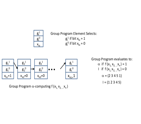
Figure 3: The form of a Group Program

We will consider predicates represented as $n$-input, single output (bounded fan-in) circuits of AND($\wedge$ two-input), OR($\vee$ two-input) and NOT($\neg$ single input) gates. Our definition of the depth of a circuit is slightly non-standard in that we ignore NOT($\neg$) gates. This is because of the Barrington Transform (to be elaborated below) which transforms a circuit into a group progam whose length depends only on the depth of the circuit in terms of AND($\wedge$) and OR($\vee$) gates.

Definition 7 (Depth of a Circuit).

The depth of a circuit is defined to be the number of AND and OR gates in the longest path from an input to the output. (NOT gates do not count towards depth).

In his seminal paper [B89], on the way to showing that $\mathsf{NC^{1}}$  is computable by fixed-width branching programs, Barrington showed that any logarithmic-depth circuit can be transformed into a polynomial-length group program - a transformation we term the Barrington Transform.

Theorem 8 (Barrington Transform).

Any circuit of depth $d$ can be transformed into a group program of length $4^{d}$ that $\alpha$-computes the same function as the circuit.

For the sake of completeness we present the proof in Appendix A.1. The proof, presented as a series of lemmas, details the Barrington Transform showing how to transform a circuit into a group program. This treatment is directly based on [Viola09].

It follows from Theorem 8 that the Barrington Transform transforms any $n$-input single output circuit of depth $\kappa\lg n$ into a group program of length $n^{2\kappa}$ where $\kappa$ is a constant.

We will be using an extension of the notion of randomized encodings [IK00, AIK05, A11] that played a significant role in the breakthrough showing the feasibility of cryptography in $\mathsf{NC^{0}}$  [AIK04]. First, we give the definition of randomized encodings.

Definition 9 (Randomized encoding).

A function $f(x)$ is said to have a randomized encoding $\hat{f}(x,r)$, where $r$ is a random string, if there exist two efficiently computable (deterministic, polynomial-time) algorithms REC and SIM such that

Correctness $\forall x,r$, given $\hat{f}(x,r)$ REC recovers $f(x)$, i.e. REC$(\hat{f}(x,r))=f(x)$ .

Security $\forall x$, given $x$ and $r^{\prime}$ (random coins), SIM produces a distribution identical to $\hat{f}(x,r)$, i.e., the distribution of SIM$(x,r^{\prime})$ is identical to the distribution of $\hat{f}(x,r)$.

The above definition will make it easier to comprehend the definition of a 2-decomposable randomized encoding. We believe that, though natural in the context of 2-party secure computation, this is the first time this definition is appearing explicitly in the literature. A stronger definition of decomposable randomized encodings has appeared before [IKOS08, IKOS09] and the notion of 2-decomposable randomized encodings is implicit in prior works, including [FKN94].

Definition 10 (2-decomposable Randomized encoding).

A function $f(x,y)$ is said to have a 2-decomposable randomized encoding $\langle\hat{f}_{1}(x,r),\hat{f}_{2}(y,r)\rangle$, where $r$ is a (shared) random string, if there exist two efficiently computable (deterministic, polynomial-time) algorithms REC and SIM such that

Correctness $\forall x,y,r$, given $\langle\hat{f}_{1}(x,r),\hat{f}_{2}(y,r)\rangle$ REC recovers $f(x,y)$, i.e., REC$(\langle\hat{f}_{1}(x,r),\hat{f}_{2}(y,r)\rangle)=f(x,y)$.

Security $\forall x,y$, given $x,y$ and $r^{\prime}$ (random coins), SIM produces a distribution identical to $\langle\hat{f}_{1}(x,r),\hat{f}_{2}(y,r)\rangle$, i.e., the distribution of SIM$(x,y,r^{\prime})$ is identical to the distribution of $\langle\hat{f}_{1}(x,r),\hat{f}_{2}(y,r)\rangle$.

The schemes presented in this paper rely crucially on the model and construction presented in [FKN94]. We define the FKN model and show how protocols for it are essentially equivalent to 2-decomposable randomized encodings.

Definition 11 (FKN model).

The 3 parties in the FKN model and their states of knowledge are captured in Figure 4. There is a single round of communication where Alice and Bob each send a private message ($E_{r}(x)$ and $E_{r}(y)$, respectively) to Carol who is then able to efficiently compute the publicly known function $f(x,y)$ such that

Correctness $\forall x,y$, and $r$, given the encrypted messages $E_{r}(x),E_{r}(y)$ Carol computes $f(x,y)$ correctly all the time.

Security $\forall x,y$, and $r$, given the encrypted messages $E_{r}(x),E_{r}(y)$ Carol learns nothing whatsoever about $x,y$ (other than the value of $f(x,y)$).

Figure 4: FKN model

Lemma 12 (Equivalence of FKN and 2-decomposable randomized encoding).

There is a 1-1 isomorphism between protocols for the FKN model and 2-decomposable randomized encodings.

Proof.

We will first see that a 2-decomposable randomized encoding of the function $f(x,y)$ gives rise to a protocol for the FKN model. Let Alice compute and send $\hat{f}_{1}(x,r)$ to Carol while Bob computes and send $\hat{f}_{2}(y,r)$ to Carol. From the Correctness property it follows that Carol can run REC$(\langle\hat{f}_{1}(x,r),\hat{f}_{2}(y,r)\rangle)$ to compute $f(x,y)$ correctly all the time. And from the Security property we get that Carol learns nothing but the value $f(x,y)$.

Similarly, given a protocol for the FKN model that computes the publicly known function $f(x,y)$ it is easy to see that the Correctness and Security properties carry over by setting $E_{r}(x)=\hat{f}_{1}(x,r)$ and $E_{r}(y)=\hat{f}_{2}(x,r)$. ∎

We present the definition of a Universal Function below.

Definition 13 (Universal Function).

A Universal Function $\mathcal{UF}$ has two inputs $x$ and $y$ where $y$ is the encoding of a function for which $x$ is a suitable input. The output of $\mathcal{UF}(x,y)$ is defined to be $y(x)$.

One can similarly define Universal Circuits which are similar to Universal Functions except that they work with encoding of circuits and simulate circuits.

Definition 14 (Universal Circuit).

A Universal Circuit $\mathcal{UC}$ has two inputs $x$ and $y$ where $y$ is the encoding of a circuit for which $x$ is a suitable input. The output of $\mathcal{UC}(x,y)$ is defined to be $y(x)$, in other words the Universal Circuit outputs the result obtained from simulating function $y$ on input $x$. (Universal Circuits are the circuit equivalent of Universal Turing Machines).

The central idea of this paper is to bypass Universal Circuits so we will not be utilizing this definition except to explain (in Section 3) how it is that we pick up efficiency gains by avoiding them.

One can naturally apply the notion of a 2-decomposable randomized encoding to a universal function $f(x,y)=y(x)$.

And analogous to the correspondence expressed in Lemma 12 we have the following correspondence.

Lemma 15 (Equivalence of C-CBPS and 2-decomposable randomized encoding of universal functions).

There is a 1-1 isomorphism between protocols for the C-CBPS model and 2-decomposable randomized encodings of universal functions.

Proof.

The proof is very similar to that of Lemma 12 and so we provide only the key aspects of the correspondence as the details are straightforward. $x,y$ correspond to $\mathfrak{m},\mathfrak{P}$ respectively. $\hat{f}_{1}(x,r),\hat{f}_{2}(y,r)$ correspond to $E_{r}(\mathfrak{m}),E_{r}(\mathfrak{P})$ respectively. And the Correctness and Security properties carry over in a direct way. ∎

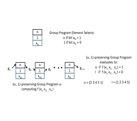
Figure 5: The form of a $(\alpha,1)$-preserving Group Program

We now present some definitions that clarify the “fixed structure” trick alluded to earlier, and how it relates to 2-decomposable randomized encodings of universal functions. The following definition of a $(\alpha,1)$-preserving group program is presented in visual form in Figure 5.

Definition 16 ($(\alpha,1)$-preserving group programs).

An $(\alpha,1)$-preserving group program of length $L$ is $(g_{1},g_{2},\ldots,g_{L+1})$, $(k_{1},k_{2},\ldots,k_{L})$ where for any $i$: $g_{i}\in S_{5}$ and $k_{i}\in\{1,\ldots,n\}$. We say that this $(\alpha,1)$-preserving group program $\alpha$-computes $f:\{0,1\}^{n}\rightarrow\{0,1\}$ if $\forall x$,

$$f(x)=1\Rightarrow(\prod^{\ell}_{i=1}g_{i}\cdot\alpha^{x_{k_{i}}})g_{L+1}=\alpha$$

$$f(x)=0\Rightarrow(\prod^{\ell}_{i=1}g_{i}\cdot\alpha^{x_{k_{i}}})g_{L+1}=1_{S_{5}};$$

which we can write compactly as $\forall x:(\prod^{\ell}_{i=1}g_{i}\cdot\alpha^{x_{k_{i}}})g_{L+1}=\alpha^{f(x)}$.

Definition 17 (Index sequence of an $(\alpha,1)$-preserving group program).

Given $(g_{1},g_{2},\ldots,g_{L+1})$, $(k_{1},k_{2},\ldots,k_{L})$, an $(\alpha,1)$-preserving group program of length $L$, its index sequence is $(k_{1},k_{2},\ldots,k_{L})$.

Analogous to Theorem 8 we have

Theorem 18 ($(\alpha,1)$-preserving Barrington Transform).

Any circuit of depth $d$ can be transformed into a $(\alpha,1)$-preserving group program of length $4^{d}$ that $\alpha$-computes the same function as the circuit.

For the sake of completeness we present the proof in Appendix A.2.

The definition of a fixed structure group program given below is crucial to improving the efficiency of the ideas presented in this paper and making them practical.

Definition 19 (Fixed structure group program).

If a class of functions (say, the class of $n$-input single output functions computable by circuits of depth $\kappa\lg n$) can all be transformed into $(\alpha,1)$-preserving group programs with the exact same index sequence (and hence the exact same length) then the resulting class of group programs is said to have a fixed structure. In a slight abuse of language we refer to the class itself as a fixed structure group program.

3 Overview

Before explaining the bottleneck that this paper has overcome we first briefly sketch the protocol for the FKN model presented in [FKN94] for publicly known functions $f(x,y)$ computable as logarithmic-depth circuits. The group program equivalent of $f$ is computed (using Barrington’s Transform [B89]) by both Alice and Bob from the corresponding circuit. Each of them instantiates their share of the group program based on their respective input ($x$ for Alice and $y$ for Bob). Then each of them blinds their share in coordinated fashion using the shared randomness. Finally, each of Alice and Bob sends their respective blinded shares to Carol who puts them together to form the final blinded sequence whose value she computes to obtain $f(x,y)$. See Figure 6. What [FKN94] essentially demonstrate is the construction of a 2-decomposable randomized encoding $\hat{f}$ of $f$, as elaborated in Lemma 12. Of course, the notion of 2-decomposable randomized encodings arose much later in the work of Ishai and Kushilevitz [IK00, IKOS08, IKOS09], but it gives us a convenient language to think about such protocols. The individual shares, constructed and, sent to Carol by Alice and Bob are just the two parts of the 2-decomposable randomized encoding, namely $\hat{f}_{1}(x,r)$ and $\hat{f}_{2}(y,r)$. REC guarantees that Carol is able to learn $f(x,y)$ while SIM guarantees that he learns nothing beyond that.

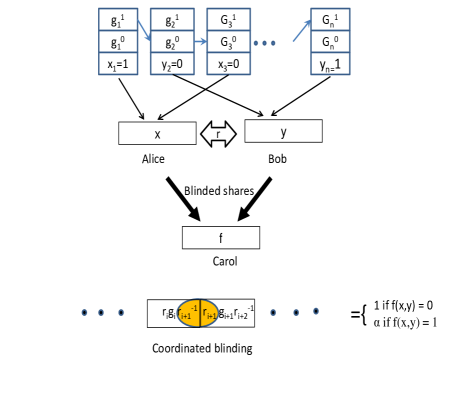
Figure 6: Protocol for FKN model, see [FKN94].

Now, we explain the universal circuits bottleneck that we claim to have overcome. Recall that in our (C-CBPS) setting $f$ is not just any function but it is a universal function where $f(x,y)=y(x)$. The term universal comes from the fact that $f$ is effectively simulating $y$ on $x$ and so the natural question arises - how efficiently can this simulation be done? In other words, given that we are restricted to have only polynomial-size group programs, what restriction does this put on the class of functions represented by $y$? The best known construction of universal circuits is due to Valiant [V76] who shows that if $y$ were a circuit of size $s$ and depth $d$ then it must satisfy $d\log s=O(\log n)$ (for the resulting Barrington Transform to produce a polynomial-length group program). Observe that this constraint on $d$ and $s$ automatically prevents $y$ from representing circuits in $\mathsf{NC^{1}}$because $s\geq d$ and hence $d$ is forced to be $o(\log n)$. Sanders, Young and Yung [SYY99] who utilize Valiant’s universal circuits construction, mention that $y$ could be the class of functions represented by circuits of depth $\sqrt{\log n}$ and size $2^{\sqrt{\log n}}$ - note that this is believed to be a strict subset of the class of predicates in $\mathsf{NC^{1}}$.

Our main contribution is in showing how we can bypass the universal circuits bottleneck and instead use group programs to improve the efficiency of simulation. We present two main constructions. The first, UGP-Match, which is primarily of theoretical interest, shows how we can handle all of $\mathsf{NC^{1}}$by encoding the subscriber’s predicate as a group program (using the Barrington Transform) and constructing a universal group program using the Barrington Transform (again). This construction has a conceptually clean proof but it is impractical since the double invocation of the Barrington Transform results in a final group program whose length is a very high-degree polynomial in $n$. Our second construction, FSGP-Match, which is potentially practical, uses a fixed structure trick to avoid one invocation of the Barrington Transform. Rather than construct a universal group program using the Barrington Transform we directly construct a fixed structure group program, which in essence is a universal group program but much more economical length-wise. By avoiding the inefficiencies arising from use of the Barrington Transform we obtain a final group program whose length is a relatively low-degree polynomial in $n$. In this second construction of FSGP-Match we need a special group program - the selector group program - which we construct by applying the Barrington Transform to a selector circuit. We also show how an additional optimization can be achieved by hand-crafting the the selector group program to obtain our most efficient construction OFSGP-Match.

4 Protocols and proofs

4.1 UGP-Match

As explained in Section 3 the main idea in the UGP-Match construction is to use the Barrington Transform to encode the predicate $\mathfrak{P}$ (which is representable as a circuit in $\mathsf{NC^{1}}$) as a polynomial-length group program that indexes into the metadata bits $\mathfrak{m}$. The (publicly known) circuit $f$ in the protocol for the FKN model [FKN94] (see Figure 6) is chosen to be such that at the lowest level it first selects the appropriate group program element based on the index and value of the corresponding bit in $\mathfrak{m}$ and having selected all the group program elements it then multiplies them together using a standard divide and conquer or balanced binary tree based approach, see Figure 7. In a nutshell, UGP-Match uses the protocol from [FKN94] for the FKN model, with $f$ being a circuit that takes as input the metadata $\mathfrak{m}$ and the predicate $\mathfrak{P}$ encoded as a group program and outputs the result of simulating $\mathfrak{P}$ on $\mathfrak{m}$. We present UGP-Match more formally below. We refer to the circuit representing $f$ as the UGP-Match Circuit. We refer to the final group program that the broker assembles as the Universal Group Program because it is essentially a Group Program that simulates the group program representing $\mathfrak{P}$.

UGP-Match

1. The publisher and subscriber register with the broker the precise form of their inputs. In particular the publisher must specify the number $n$ of bits of $\mathfrak{m}$ the meta-data (if there are fewer relevant bits, the remaining bits can be padded with dummy bits). And the subscriber specifies $L=n^{2\kappa}$ the length of the group program (in terms of number of group element pairs (not bits) along with the bit of $\mathfrak{m}$ that each group element pair is dependent on). As before the group program can be padded with dummy pairs if there are fewer relevant pairs. We may assume that everybody is coordinated on the choice of the non-solvable group in which to carry out their computations, say $S_{5}$, the (symmetric) group of permutations on $5$ elements, which itself is a group with $120$. For the purpose of this specific cprotocol we can assume each element is specified in unary using $5$ bits so that any given element of the group is specified using $5\times 5=25$ bits.

2. The broker now computes the UGP-Match Circuit $f$ (which is essentially a Select block followed by a divide-and-conquer Multiply block, see Figure 7. It then applies the Barrington Transform to create the corresponding group program. Each group element pair in this group program is dependent either on a subscriber bit or on a publisher bit. The broker hands back the entire group program to both the publisher and the subscriber.

3. The publisher and subscriber know which pairs belong to each of them. They have already coordinated their pre-shared randomness. Depending on the value of their individual bit they pick the corresponding element of the pair and then blind it appropriately. They then give their respected blinded elements to the broker.

4. The broker puts all the blinded elements together in the right sequence and multiplies them. If he gets $1$ he forwards along the (encrypted) data from the publisher to the subscriber, else he withholds it.

Figure 7: UGP-Match Circuit

Theorem 20.

Given metadata of size at most $n$ and predicate of depth at most $\kappa\lg n$, UGP-Match is an information-theoretically secure protocol for the C-CBPS model with complexity $\tilde{O}(n^{20\kappa+2}$.

Proof.

The proof that UGP-Match is correct and secure follows directly from the proof in [FKN94] for the FKN model.

All that remains to do is to bound the complexity of UGP-Match. We now provide a detailed description of the UGP-Match Circuit $f$. See Figure 7. This circuit takes in as input $\mathfrak{m}$ and the bit-representation of the group program obtained from applying the Barrington Transform (see Theorem 8) to $\mathfrak{P}$. The group program is a sequence of $L=n^{2\kappa}$ group program elements each of which is two group elements and an index (into $\mathfrak{m}$. We represent the group elements which are permutations of $S_{5}$ in unary, e.g., we would represent the permutation $(23451)$ as the bit sequence $00010\;00100\;01000\;10000\;00001$ (the spacings are placed for convenience of reading). We note that this is not the most economical representation in terms of bit-length but what we are ultimately looking to minimize is the length of the final group program, i.e. the depth of the UGP-Match Circuit and for that purpose this representation is close to optimal. Each of the indices in binary is represented using $\lg n$ bits. The UGP-Match Circuit is a Select block followed by a divide-and-conquer Multiply block. In the Select block, corresponding to each group program index the value of the bit of $\mathfrak{m}$ is extracted using a mux (multiplexer, see [WikiMux]) which is a circuit of depth $\lg n+\lg\lg n$. The corresponding group program element is then selected using a circuit of depth $2$. Multiplying two group program elements takes a circuit of depth $5$ and hence the Multiply block has depth $(5\times 2\kappa)\lg n$ (recall that the group program $\mathfrak{P}$ has length $n^{2\kappa}$). Thus the total depth of the UGP-Match Circuit is $(10\kappa+1)\lg n+\lg\lg n+2$. The Barrington Transform (see Theorem 8 of UGP-Match Circuit gives us a final group program under the FKN model of length $\tilde{O}(n^{20\kappa+2})$.

∎

Corollary 21.

UGP-Match is an efficient and secure protocol for matching any predicate in $\mathsf{NC^{1}}$.

4.2 Fixed Structure Group Programs

We now state and prove the key lemma concerning fixed structure group programs.

Lemma 22 (Fixed structure programs yield 2-decomposable randomized encodings of universal functions).

Fixed structure programs are convertible to 2-decomposable randomized encodings of universal functions with no loss of efficiency.

Proof.

The conversion of a fixed structure program to a 2-decomposable randomized encodings of universal functions is fairly straightforward involving instantiation and coordinated blinding.

Consider a class of predicates $\mathfrak{P}$ convertible to fixed structure group programs. Let $(g_{1},g_{2},\ldots,g_{L+1}),$ $(k_{1},k_{2},\ldots,k_{L})$ be the fixed structure group program, i.e., a $(\alpha,1)$-preserving group program with a fixed index sequence (the index sequence is the same independent of the specific function that the group program is computing though the interstitial group elements $(g_{1},g_{2},\ldots,g_{L+1})$ would depend on the specific function). We now need to demonstrate two functions $\hat{f}_{1}(\mathfrak{m},r)$ and $\hat{f}_{2}(\mathfrak{P},r)$ satisfying the requirements of Definition 10, with the additional constraint of universality, namely that $f(\mathfrak{m},\mathfrak{P})=\mathfrak{P}(\mathfrak{m})$.

Given a specific instance of metadata $\mathfrak{m}$ the function $\hat{f}_{1}$ first selects $\alpha$ or $1$ as appropriate for each of the index sequence pairs; note that this is done independent of the specific predicate $\mathfrak{P}$. Then $\hat{f}_{1}$ blinds the resulting sequence using the randomness $r$. Similarly, depending on the specific predicate $\mathfrak{P}$ $\hat{f}_{2}$ converts to the fixed structure group program and gets a specific instantiation of the interstitial group elements $(g_{1},g_{2},\ldots,g_{L+1})$. Then this sequence is blinded by $\hat{f}_{2}$ using $r$. Observe that the fixed structure is crucial for the construction of $\hat{f}_{1}$ so that it is independent of $\mathfrak{P}$. u

It remains to prove Correctness and Security as per Definition 10. First, the existence of REC and Correctness follows because of the appropriate cancelation of the blinders and so $\mathfrak{P}(\mathfrak{m})$ can be recovered exactly from multiplying the elements of the final assembled group program. Next, the existence of SIM and Security - observe that independent of the specific instance the broker receives shares of the same form from both publisher and subscriber and by Lemma 5 (Blinding Lemma) these shares are uniformly distributed over all possible sequences with same final value and therefore SIM can generate the outputs with the same distribution as $\hat{f}_{1}$ and $\hat{f}_{2}$ by generating all but one element of the sequence completely and uniformly at random, then generating the last element so that the value of the sequence is the given final value, and then splitting the group program into the two parts corresponding to $\hat{f}_{1}$ and $\hat{f}_{2}$. ∎

Observe that an implication of the above Lemma is that the fixed structure of the group program implicitly encodes a universal function.

The below corollary follows from the two lemmas, Lemma 22 and 15, since 2-decomposable randomized encodings of universal functions are isomorphic to protocols for the C-CBPS model.

Corollary 23.

Fixed structure programs yield secure C-CBPS protocols with no loss of efficiency.

4.3 FSGP-Match

With Lemma 22 and Corollary 23 in hand, all we need to do is to demonstrate a fixed structure group program of the right complexity. We give an intuitive description of the main idea. Applying the $(\alpha,1)$-preserving Barrington Transform to the predicate $\mathfrak{P}$ yields an $(\alpha,1)$-preserving group program but not a fixed structure group program because the index sequence would vary depending on the predicate $\mathfrak{P}$. So, then we substitute each instance of a group program pair in this group program by a fixed $(\alpha,1)$-preserving group program block we call the Fixed Selector Group Program. This creates a fixed structure. And by padding appropriately we can fix the length to be independent of the inputs as well. It remains to describe the Fixed Selector Group Program. The Fixed Selector Group Program is obtained by applying an $(\alpha,1)$-preserving Barrington Transform to the Fixed Selector Circuit. Figure 8 is a visual description of the Fixed Selector Circuit. The Fixed Selector Circuit is an OR of ANDs. It has one AND gate for each bit of the metadata $\mathfrak{m}$ as input. The other input to the AND gate is a “new” bit under the control of the subscriber. Since the subscriber knows the predicate $\mathfrak{P}$ it knows exactly which bit of the input ($\mathfrak{m}$) it needs in that particular block (based on the index of the group program pair that the block is replacing). Once the subscriber instantiates these bits approrpriately and blinds then the Fixed Selector Group Program is just a block with a fixed index sequence since all the dependence on the predicate $\mathfrak{P}$ is factored into the interstitial group elements. Thus the overall index sequence is fixed. Note that for blocks in the padding the subscriber can set all new bits to $0$ thus effectively reducing the padding part of the group program to a no-op, something that evaluates to $1$.

Figure 8: Fixed Selector Circuit

FSGP-Match

1. The publisher and subscriber register with the broker the precise form of their inputs. In particular the publisher must specify the number $n$ of bits of $\mathfrak{m}$ the meta-data (if there are fewer relevant bits, the remaining bits can be padded with dummy bits). And the subscriber specifies $D=2\kappa\lg n$ the maximal depth of the predicate $\mathfrak{P}$.

2. The broker now comutes the form of the fixed structure group program by applying the $(\alpha,1)$-preserving Barrington Transform to any circuit of depth $D$ to create the corresponding $(\alpha,1)$-preserving group program. Again, only the form of the group program is relevant at this stage, not the values of the specific interstitial group elements or indices in the index sequence. It then replaces each group program pair with the Fixed Selector Group Program and returns the entire composite group program back to the publisher and subscriber. At this point the values of the interstitial group elements do not matter but the index sequence, which is fixed, does matter. The program is an $\alpha,1)$-preserving group program with indices that index into the metadata bits.

3. The publisher selects one of $\alpha$ or $1$ depending on the value of the corresponding metadata bit for each group program pair, blinds them and sends back to the broker. The subscriber, applies the $(\alpha,1)$-preserving Barrington Transform to the specific instance $\mathfrak{P}$ to get the concrete values for the interstitial group elements, appropriately sets the “new” bits for the Fixed Selector Group Program blocks, and blinds the entire sequence and sends to the broker.

4. The broker puts all the blinded elements together in the right sequence and multiplies them. If he gets $1$ he forwards along the (encrypted) data from the publisher to the subscriber, else he withholds it.

Theorem 24.

Given metadata of size at most $n$ and predicate of depth at most $\kappa\lg n$, FSGP-Match is an information-theoretically secure protocol for the C-CBPS model with complexity $4n^{2\kappa+2}$.

Proof.

FSGP-Match is obtained by applying the $(\alpha,1)$-preserving Barrington Transform to the predicate $\mathfrak{P}$ to yield an $(\alpha,1)$-preserving group program where each instance of a group program pair is substituted by the Fixed Selector Group Program. It is clear that FSGP-Match produces a fixed structure group program and hence it follows from Lemma 22 that it is correct and secure.

All that remains to do is to bound the complexity of FSGP-Match. Recall that group program pair in the group program (of length $n^{2\kappa}$ is substituted by the Fixed Selector Group Program. The Fixed Selector Group circuit (see Figure 8) has depth $1+\lg n$ and hence the resulting Fixed Selector Group Program has length $4n^{2}$ which means that the final group program has a length $4n^{2}\times n^{2\kappa}=4n^{2\kappa+2}$. ∎

4.4 OFSGP-Match

OFSGP-Match is basically FSGP-Match with the additional innovation being that we use an Optimized Fixed Selector Group Program. See Figure 9.

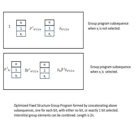
Figure 9: (Hand) Optimized Fixed Selector Group Program

Theorem 25.

Given metadata of size at most $n$ and predicate of depth at most $\kappa\lg n$, OFSGP-Match is an information-theoretically secure protocol for the C-CBPS model with complexity $2n^{2\kappa+1}$.

Proof.

The proof is similar to the proof of Theorem 24 so we do not repeat it.

The Optimized Fixed Selector Group Program (see Fig. 9) has length $2n$ which means that the final group program has a length $2n\times n^{2\kappa}=2n^{2\kappa+1}$. ∎

5 Implementation and Performance

We implemented all three of our protocols in Java. We will spare the reader the details of the code. As has already been explained the protocols are conceptually straightforward. The only protocol that was somewhat performant was OFSGP-Match. In particular, we considered the Hamming problem as that is representative of a typical function in the context of publish/subscribe. The publisher and the subscriber each have a private bit-vector of $n$ bits. They wish to compute a secure Hamming match, i.e., given a common threshold level (between $0$ and $\log_{2}n$) they wish to exchange the actual content iff the Hamming distance between their respective vectors exceeds the threshold. The bottleneck from a computational standpoint is the cost of computing a match at the broker, which is basically the length of the resulting group program. Since, in our setting the subscribers submit predicates, we have our subscriber submit the Hamming distance circuit with its own bit-vector and the threshold hard-coded into it.

Our match algorithm implemented as a circuit, essentially, involved computing the difference vector of the two vectors, then sorting the bits using a Bose-Nelson sorting network [BN62], and outputting the threshold bit as the match. We used a Bose-Nelson circuit because they have the shortest depth (i.e. best constants) for small depths (even though AKS sorting networks [AKS83] are asymptotically optimal - depth $O(\log n)$ - instead of $O(\sqrt{(}n))$ for Bose-Nelson). We implemented the above match algorithm on a 3GHz quad-core i7 laptop. Our goal was to find the largest $n$ for which the match could be computed under 1s. The results are presented in Table 2 in Appendix B. Here $n$ is the length of the bit-vectors. $d$ is the depth of the resulting ciruit and the final column shows the length of the resulting OFSGP-Match sequence. The main takeaway is that even our best scheme becomes unusable for a relative simple function such as the Hamming distance once the bit vectors get to over 16 bits in length.

6 Conclusion

We started out on a research plan to achieve secure publish/subscribe at line speeds. Though we did not reach our goal this paper reports on the substantial progress we achieved - namely information-theoretically secure publish/subscribe for predicated in $\mathsf{NC^{1}}$. On the theoretical front we achieved a level of expressivity that had not been previously attained and on the practical front we made a substantial advance towards a practical scheme. Our protocols have the benefit of being conceptually clean and simple, so simple that we can capture their complexity without even employing the big-Oh notation, see Table 1 . Going forward, the main open question is to come up with a much faster protocol, potentially one that will scale at wireline speeds (Gbps).

Appendix A Barrington Transform

A.1 Barrington Transform

We present the proof of Theorem 8 based on the treatment in [Viola09]. (Note that the statement of the theorem is true for any cycle $\alpha$ and not just the specific cycle $(23451)$.

Proof.

We present the proof as a series of lemmas.

Lemma 26 (The cycle does not matter).

Let $\alpha,\beta\in S_{5}$ be two cycles, let $f:\{0,1\}^{n}\rightarrow\{0,1\}$. Then f is $\alpha$-computable with length $\ell$ $\Leftrightarrow$ f is $\beta$-computable with length $\ell$.

Proof.

First observe that $\exists\rho_{\alpha\beta}\in S_{5}$ such that $\alpha=\rho_{\alpha\beta}^{-1}\beta\rho_{\alpha\beta}$.

To see this let

$$\alpha=(\alpha_{1},\alpha_{2},...,\alpha_{5})_{\mbox{cycle}}$$

$$\beta=(\beta_{1},\beta_{2},...,\beta_{5})_{\mbox{cycle}}$$

$$\rho_{\alpha\beta}:=(\alpha_{1}\rightarrow\beta_{1},\alpha_{2}\rightarrow\beta_{2},...,\alpha_{5}\rightarrow\beta_{5}).$$

(With $\alpha=(23451)$ and $\beta=(35421)$ we get $\rho_{\alpha\beta}=(13425),\rho_{\alpha\beta}^{-1}=(14235)$.

Suppose that $(g_{1}^{0},...,g_{\ell}^{0})(g_{1}^{1},...,g_{l}^{1})(k_{1},...k_{\ell})$ $\beta$-computes $f$; we claim that $(\rho_{\alpha\beta}^{-1}g_{1}^{0},...,g_{\ell}^{0}\rho_{\alpha\beta})(\rho_{\alpha\beta}^{-1}g_{1}^{1},...,g_{\ell}^{1}\rho_{\alpha\beta})$ (with the same indices $k_{i}$) $\alpha$-computes $f$. To see this, note that

$$\prod^{\ell}_{i=1}g_{i}^{x_{k_{i}}}=1_{G}\Rightarrow\rho_{\alpha\beta}^{-1}\prod^{l}_{i=1}g_{i}^{x_{k_{i}}}\rho=\rho^{-1}\cdot\rho_{\alpha\beta}=1,$$

$$\prod^{\ell}_{i=1}g_{i}^{x_{k_{i}}}=\beta\Rightarrow\rho_{\alpha\beta}^{-1}\prod^{l}_{i=1}g_{i}^{x_{ki}}\rho=\rho^{-1}\beta\rho_{\alpha\beta}=\alpha.$$

∎

Lemma 27 ($f\Rightarrow 1-f$).

If $f:\{0,1\}^{n}\rightarrow\{0,1\}$ is $\alpha$-computable by a group program of length $\ell$, so is $1-f$.

Proof.

First apply the previous lemma to $\alpha^{-1}$-compute $f$. Then multiply last group elements $g^{0}_{\ell}$ and $g^{1}_{\ell}$ in the group program by $\alpha$. (Note that $\alpha^{-1}=(51234)$.) ∎

Lemma 28 ($f,g\Rightarrow f\wedge g$).

If $f$ is $\alpha$-computable with length $\ell$ and $g$ is $\beta$ computable with length $\ell$ then ($f\wedge g$) is ($\alpha\beta\alpha^{-1}\beta^{-1}$)-computable with length $4\ell$.

Proof.

Concatenate $4$ programs: ($\alpha$-computes $f$, $\beta$-computes $g$, $\alpha^{-1}$-computes $f$, $\beta^{-1}$-computes $g$). (f(x)=1)$\wedge$ (g(x)=1)$\Rightarrow$ concatenated program evaluates to ($\alpha\beta\alpha^{-1}\beta^{-1}$); but if either $f(x)=0$ or $g(x)=0$ then the concatenated program evaluates to $0$. For example, if $f(x)=0$ and $g(x)=1$ then the concatenated program gives $1\cdot\beta\cdot 1\cdot\beta^{-1}=1$. ∎

It only remains to see that we can apply the previous lemma while still computing with respect to a cycle.

Lemma 29.

$\exists\alpha,\beta$ cycles such that $\alpha\beta\alpha^{-1}\beta^{-1}$ is a cycle.

Proof.

Let $\alpha:=(23451)$, $\beta:=(35421)$, we can check $\alpha\beta\alpha^{-1}\beta^{-1}=\gamma=(35214)$ is a cycle. ∎

The proof of the theorem follows by induction on $d$ using previous lemmas. ∎

A.2 $(\alpha,1)$-preserving Barrington Transform

The proof of Theorem 18 is basically the same as the proof of Theorem 8 with minor modifications to account for the fact that we are now transforming the circuit into an $(\alpha,1)$-preserving group program.

Proof.

As before we present the proof as a series of lemmas.

Lemma 30 (The cycle does not matter).

Let $\alpha,\beta\in S_{5}$ be two cycles, let $f:\{0,1\}^{n}\rightarrow\{0,1\}$. Then f is $\alpha$-computable with length $\ell$ $\Leftrightarrow$ f is $\beta$-computable with length $\ell$.

Proof.

The proof is similar to that of Lemma 26. Let $\alpha,\beta\rho_{\alpha\beta}\in S_{5}$ be as in that lemma. Suppose that $(g_{1},g_{2},\ldots,g_{L+1})$ $(k_{1},k_{2},\ldots,k_{L})$ $\beta$-computes $f$ then it follows, in straightforward fashion that $(\rho_{\alpha\beta}^{-1}g_{1},g_{2},\ldots,g_{L+1}\rho_{\alpha\beta})$ $(k_{1},k_{2},\ldots,k_{L})$ $\alpha$-computes $f$. ∎

Lemma 31 ($f\Rightarrow 1-f$).

If $f:\{0,1\}^{n}\rightarrow\{0,1\}$ is $\alpha$-computable by a group program of length $\ell$, so is $1-f$.

Proof.

First apply the previous lemma to $\alpha^{-1}$-compute $f$. Then multiply the last group elements $g_{L}$ group program by $\alpha$. ∎

Lemma 32 ($f,g\Rightarrow f\wedge g$).

If $f$ is $\alpha$-computable with length $\ell$ and $g$ is $\beta$ computable with length $\ell$ then ($f\wedge g$) is ($\alpha\beta\alpha^{-1}\beta^{-1}$)-computable with length $4\ell$.

Proof.

The proof of this Lemma is identical to the proof of Lemma 28. ∎

The proof of the theorem follows by induction on $d$ using previous lemmas. and Lemma 29. ∎

Appendix B Hamming distance - Performance

$n$ - bit-vector length	$d$ - circuit depth	OFSGP-Match - sequence length
$2$	$5$	$4096$
$3$	$8$	$393216$
$4$	$8$	$524288$
$5$	$12$	$1.68*10^{8}$
$6$	$12$	$2.01*10^{8}$
$7$	$13$	$9.4*10^{8}$
$8$	$13$	$1.07*10^{9}$
$9$	$16$	$7.73*10^{10}$
$10$	$16$	$8.59*10^{10}$
$11$	$16$	$9.45*10^{10}$
$12$	$16$	$1.03*10^{11}$
$13$	$16$	$1.12*10^{11}$
$14$	$16$	$1.2*10^{11}$
$15$	$16$	$1.29*10^{11}$
$16$	$16$	$1.37*10^{11}$

Table 2: Length of group program for computing Hamming distance.