Local Density of States in a Helical Tomonaga-Luttinger Liquid of Loop and Josephson Junction Geometries

Abstract

The local density of states (LDOS) in a one-dimensional helical channel of finite length is studied within a Tomonaga-Luttinger model at zero temperature. Two particular cases of loop and Josephson junction geometries are considered. The LDOS, as a function of energy $\omega$ measured from the Fermi level, consists of equally spaced spikes of the $\delta$-function type, and electron-electron interactions modify their relative height. It is shown that, in the loop geometry, the height of spikes decreases as $\omega\to 0$ everywhere in the system. It is also shown that, in the Josephson junction, the behavior of the LDOS significantly depends on the spatial position. At the end points of the junction, the height increases as $\omega\to 0$ and its variation is more pronounced than that in the loop case. Away from the end points, the height of spikes shows a non-monotonic $\omega$-dependence, which disappears in the long-junction limit.

1 Introduction

The existence of a one-dimensional (1D) edge channel with a linear energy dispersion is the most notable property of quantum spin Hall insulators. [1, 2, 3, 4, 5] This 1D channel is called helical as it hosts up-spin and down-spin electrons moving in opposite directions. As a consequence of the time-reversal invariance of quantum spin Hall insulators, these two branches are connected by time-reversal symmetry. This forbids impurity-induced single-particle backward scattering. The absence of backward scattering is a remarkable property of the 1D helical channel allowing it to be free from Anderson localization.

The electron-electron interaction effect on the 1D helical channel has been studied in Refs. wu and xu. It is shown that the system remains gapless even in the presence of disorder unless interactions are extraordinarily strong, and is described by the concept of a Tomonaga-Luttinger liquid. [8, 9, 10, 11, 12, 13] Since this helical liquid has only one time-reversal invariant pair of up-spin and down-spin branches moving in opposite directions, its description is simpler than that of an ordinary spin-full Tomonaga-Luttinger liquid. Hence, the 1D helical channel of quantum spin Hall insulators can be regarded as an ideal platform to examine the characteristic behavior of the Tomonaga-Luttinger liquid.

Although the 1D helical channel is most naturally realized on the edge of quantum spin Hall insulators, it has been demonstrated that the step defect on a certain surface of weak topological insulators can also host an equivalent 1D channel. [14] This channel inevitably forms a closed loop structure as discussed in Ref. yoshimura, indicating that a Tomonaga-Luttinger liquid in the loop geometry [15, 16, 17, 18, 19, 20] can be realized on a surface of weak topological insulators. The system similar to this is also realized in the Josephson junction [21, 22, 23, 24, 25, 26, 27] of a Tomonaga-Luttinger liquid, which can be made by depositing two superconductors on a quantum spin Hall insulator. In the Josephson junction, electrons near the Fermi level is effectively confined in the finite region between the superconductors. In such systems, how does the finiteness of an effective system length affect the behavior of the 1D helical channel?

In this paper, we focus on the local density of states in the 1D helical channel at zero temperature and study the finite-size effect on it combined with the effect of interactions within the Tomonaga-Luttinger liquid theory. We consider the two cases of the loop and Josephson junction geometries. If the local density of states is plotted as a function of the energy $\omega$ (measured from the Fermi level), it consists of equally spaced spikes of the $\delta$-function type, reflecting the finiteness of system length, [28] and the electron-electron interactions modify the height of these spikes. It is shown that the $\omega$-dependence of peak height is determined by the correlation exponent $K$ characterizing the strength of interactions. In the loop geometry case, the height of spikes decreases as $\omega\to 0$ everywhere in the loop. It is also shown that, in the Josephson junction case, the behavior of the local density of states significantly depends on the spatial position in the junction between two superconductors. At the end points of the junction, the height of spikes increases as $\omega\to 0$ in contrast to the loop case. Furthermore, its variation as a function of $\omega$ is much more pronounced than that in the loop case. Away from the end points, the height of spikes shows a non-monotonic $\omega$-dependence, which disappears in the limit where the system length is large enough.

In the next section, we describe a weakly interacting 1D helical channel in both the loop and Josephson junction geometries within the Tomonaga-Luttinger liquid theory. The expressions of the Hamiltonian and electron field are presented in a bosonized form. In Sect. 3, we calculate the local density of states and discuss its characteristic behaviors. The last section is devoted to the summary. We set $\hbar=1$ throughout this paper.

2 Bosonized Model

We focus on a weakly interacting 1D helical channel consisting of right-going up-spin electrons and left-going down-spin electrons. Before presenting its bosonized description, let us briefly summarize the energy spectrum of a 1D helical channel in the non-interacting limit. Hereafter, $\sigma$ is used to denote the spin directions: $\sigma=\uparrow$ for up spin and $\sigma=\downarrow$ for down spin, and the sign function $s_{\sigma}$ is defined as $s_{\sigma}=+$ ($-$) for $\sigma=\uparrow$ ($\downarrow$).

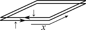
Figure 1: Schematic of the 1D helical channel consisting of right-going up-spin branch and left-going down-spin branch.

Let us first consider the 1D helical channel of length $L$ in the loop geometry (see Fig. 1). We assume that the loop encircles a magnetic flux $\phi$, which induces the Aharonov-Bohm phase

$$\chi\equiv 2\pi\frac{\phi}{\phi_{0}},$$ (1)

where $\phi_{0}=2\pi/e$ is the flux quantum. In the absence of electron-electron interactions, the electrons in this system obey the following eigenvalue equation:

$$v_{\rm F}\bigl{[}s_{\sigma}\left(-i\partial_{x}+eA_{x}\right)-k_{\rm F}\bigr{]}u_{\sigma}(x)=\epsilon u_{\sigma}(x),$$ (2)

where $v_{\rm F}$ and $k_{\rm F}$ respectively are the Fermi velocity and Fermi wave number, and $A_{x}$ is the tangential component of the vector potential. Note that the wave function satisfies the anti-periodic boundary condition $u_{\sigma}(x)=-u_{\sigma}(x+L)$ in the helical channel owing to the rotation of the spin-quantization axis. [29] If $k_{\rm F}L=2\pi\times{\rm integer}$ is assumed for simplicity, the energy eigenvalues for up-spin and down-spin electrons are given by

$$\epsilon_{\sigma}=v_{\rm F}\left(q+\frac{\pi+s_{\sigma}\chi}{L}\right),$$ (3)

where $q=2\pi n/L$ ($n=0,\pm 1,\pm 2,\dots$). The factor $\pi/L$ reflects the anti-periodic boundary condition.

We turn to the case of the Josephson junction, in which the 1D helical channel is effectively confined in the region of length $L$ by two superconductors (see Fig. 2), where the right (left) superconductor occupies the region of $x\geq L$ ($x\leq 0$). The electrons in this system obey the following eigenvalue equation: [30]

$$\left(\begin{array}[]{cc}v_{\rm F}\left(-is_{\sigma}\partial_{x}-k_{\rm F}\right)&\Delta(x)e^{i\chi(x)}\\ \Delta(x)e^{-i\chi(x)}&v_{\rm F}\left(is_{\sigma}\partial_{x}+k_{\rm F}\right)\end{array}\right)\left(\begin{array}[]{c}u_{\sigma}(x)\\ v_{\sigma}(x)\end{array}\right)$$ (8)

$$\hskip 28.45274pt=\epsilon\left(\begin{array}[]{c}u_{\sigma}(x)\\ v_{\sigma}(x)\end{array}\right),$$ (11)

where $\Delta(x)$ and $\chi(x)$, respectively, are the magnitude and phase of the pair potential in the superconductors. We assume that $\Delta(x)$ has a constant value, $\Delta_{0}$, in the region occupied by the right or left superconductor and vanishes in the region of $L>x>0$, and that $\chi(x)$ is equal to $\chi_{\rm R}$ ($\chi_{\rm L}$) in the right (left) superconductor. In the low-energy regime of $|\epsilon|<\Delta_{0}$, the energy eigenvalues for up-spin and down-spin electrons are given by

$$\epsilon_{\sigma}=v_{\rm F}\left(q+\frac{\pi+s_{\sigma}\chi}{2L_{+}}\right),$$ (12)

where $q=\pi n/L_{+}$ ($n=0,\pm 1,\pm 2,\dots$), $L_{+}=L+\xi$ with $\xi\equiv v/\Delta_{0}$ being the coherence length, and $\chi$ is the phase difference defined by $\chi\equiv\chi_{\rm R}-\chi_{\rm L}$. The effective length $L_{+}$ for electrons is slightly enlarged by the phase shift induced in Andreev reflection processes. [22, 24]

Figure 2: Schematic of the 1D helical channel on which two superconductors separated by $L$ is deposited.

Now, we present a bosonized description of a weakly interacting 1D helical channel in the two cases of the loop and Josephson junction geometries. We describe the effect of electron-electron interactions within the framework of the Tomonaga-Luttinger liquid. Generally, the bosonized Hamiltonian $H$ is decomposed into $H=H_{\rm Z}+H_{\rm NZ}$, where $H_{\rm Z}$ and $H_{\rm NZ}$ respectively describe the zero and non-zero modes. [13] The electron field $\psi_{\sigma}(x)$ is expressed as [11, 12, 15]

$$\psi_{\sigma}(x)=\frac{1}{\sqrt{2\pi\alpha}}e^{is_{\sigma}k_{\rm F}x+i\theta_{\sigma}(x)},$$ (13)

where $\alpha$ is a short distance cutoff and $\theta_{\sigma}(x)$ is the phase field. With the explicit expression of $\theta_{\sigma}(x)$ given below, we can show that the electron field satisfies the anti-commutation relation

$$\psi_{\sigma}(x)\psi_{\sigma^{\prime}}^{\dagger}(x^{\prime})+\psi_{\sigma^{\prime}}^{\dagger}(x^{\prime})\psi_{\sigma}(x)=\delta_{\sigma,\sigma^{\prime}}\delta\left(x-x^{\prime}\right)$$ (14)

for $L\geq x,x^{\prime}\geq 0$. The phase field is also decomposed into the zero and non-zero mode components as follows:

$$\theta_{\sigma}(x)=\theta_{\sigma}^{0}(x)+\frac{1}{2}\left(s_{\sigma}\theta_{+}(x)+\theta_{-}(x)\right),$$ (15)

where $\theta_{\sigma}^{0}(x)$ is the zero-mode component and $\theta_{\pm}(x)$ describes the non-zero modes. The explicit forms of the Hamiltonian and the phase field necessarily reflect its geometry, so we separately treat the two cases below. However, the correlation exponent $K$ and the renormalized velocity $v$ are commonly used in both the cases, where $K$ characterizes the strength of interactions and $K<1$ in the ordinary case of repulsive interaction. Note that $K=1$ and $v=v_{\rm F}$ in the non-interacting limit. For convenience, we here define $\gamma_{\pm}$ as

$$\gamma_{\pm}=\frac{1}{2}\left(\frac{1}{K}\pm K\right).$$ (16)

2.1 Loop geometry

With the parameters $v$ and $K$ introduced above, $H_{\rm Z}$ and $H_{\rm NZ}$ are respectively given by [13, 15]

$$H_{\rm Z} =\frac{\pi v}{2L}\left(\frac{1}{K}M^{2}+K\left(J+\frac{\chi}{\pi}\right)^{2}\right),$$ (17)

$$H_{\rm NZ} =\sum_{q>0}vq\left(\beta_{q}^{\dagger}\beta_{q}+\beta_{-q}^{\dagger}\beta_{-q}\right),$$ (18)

where $J$ and $M$ are the winding numbers satisfying the constraint that their sum must be an even integer, [15] and $\beta_{q}$ ($\beta_{q}^{\dagger}$) is the boson annihilation (creation) operator with $q=2\pi n/L$ ($n=1,2,3,\dots$). The zero-mode component of the phase field is given by

$$\theta_{\sigma}^{0}(x)=\vartheta+s_{\sigma}\varphi+\frac{\pi}{L}x\left(J+\frac{\chi}{\pi}\right)+s_{\sigma}\frac{\pi}{L}\left(x+\frac{L}{2}\right)M,$$ (19)

with $[J,\varphi]=[M,\vartheta]=i$, while the non-zero-mode component is given by

$$\theta_{+}(x) =i\sqrt{K}\sum_{q>0}\sqrt{\frac{2\pi}{Lq}}e^{-\alpha q/2}\Bigl{[}e^{-iqx}\left(\beta_{q}^{\dagger}+\beta_{-q}\right)$$

$$\hskip 99.58464pt-e^{iqx}\left(\beta_{q}+\beta_{-q}^{\dagger}\right)\Bigr{]},$$ (20)

$$\theta_{-}(x) =\frac{i}{\sqrt{K}}\sum_{q>0}\sqrt{\frac{2\pi}{Lq}}e^{-\alpha q/2}\Bigl{[}e^{-iqx}\left(\beta_{q}^{\dagger}-\beta_{-q}\right)$$

$$\hskip 99.58464pt-e^{iqx}\left(\beta_{q}-\beta_{-q}^{\dagger}\right)\Big{]}.$$ (21)

2.2 Josephson junction

The bosonized description of the Josephson junction of a spin-full Tomonaga-Luttinger liquid has been presented by several authors. [21, 22, 23, 24, 31] Applying the prescription to the helical case, we find that [27]

$$H_{\rm Z} =\frac{\pi vK}{2L_{+}}\left(N+\frac{\chi}{2\pi}\right)^{2},$$ (22)

$$H_{\rm NZ} =\sum_{q>0}vq\beta_{q}^{\dagger}\beta_{q},$$ (23)

where $q=\pi n/L_{+}$ ($n=1,2,3,\cdots$). The zero-mode component of the phase field is given by

$$\theta_{\sigma}^{0}(x)=s_{\sigma}\varphi+\frac{\pi}{L_{+}}\left(x+\frac{\xi}{2}\right)\left(N+\frac{\chi}{2\pi}\right),$$ (24)

with $[N,\varphi]=i$, while the non-zero-mode component is given by

$$\theta_{+}(x) =i\sqrt{K}\sum_{q>0}\sqrt{\frac{4\pi}{L_{+}q}}e^{-\alpha q/2}\cos q\left(x+\frac{\xi}{2}\right)\left(\beta_{q}^{\dagger}-\beta_{q}\right),$$ (25)

$$\theta_{-}(x) =\frac{1}{\sqrt{K}}\sum_{q>0}\sqrt{\frac{4\pi}{L_{+}q}}e^{-\alpha q/2}\sin q\left(x+\frac{\xi}{2}\right)\left(\beta_{q}^{\dagger}+\beta_{q}\right).$$ (26)

In contrast to the loop geometry case, $\theta_{\pm}(x)$ has a nontrivial spatial dependence as a consequence of the Andreev reflection. For example, the fluctuation of $\theta_{-}$ is strongly suppressed near both ends of the system (i.e., $x=0$ and $L$). [24, 31] This results in anomalous $x$- and $\omega$-dependences of the local density of states.

3 Local Density of States

To obtain an analytical expression of the local density of states at zero temperature, it is convenient to introduce the retarded Green’s function defined by

$$G_{\sigma}^{\rm R}(x,x^{\prime};t) =-i\Theta(t)\Bigl{[}\langle\psi_{\sigma}(xt)\psi_{\sigma}^{\dagger}(x^{\prime}0)\rangle$$

$$\hskip 56.9055pt+\langle\psi_{\sigma}^{\dagger}(x^{\prime}0)\psi_{\sigma}(xt)\rangle\Bigr{]},$$ (27)

where $\Theta(t)$ is the Heaviside step function, $\langle\cdots\rangle$ represents the average in the ground state, and

$$\psi_{\sigma}(xt)=e^{iHt}\psi_{\sigma}(x)e^{-iHt}.$$ (28)

Then, the local density of states at $x$ is expressed as

$$D_{\sigma}(x,\omega)=-\frac{1}{\pi}{\rm Im}\left\{\int_{-\infty}^{\infty}\!dt\,e^{i\omega t}G_{\sigma}^{\rm R}(x,x;t)\right\}.$$ (29)

Below, we separately treat the cases of loop and Josephson junction geometries.

3.1 Loop geometry

Using the bosonized expressions for the Hamiltonian and electron field, we obtain the retarded Green’s function as

$$G_{\sigma}^{\rm R}(x,x;t) =-i\Theta(t)\frac{1}{2\pi\alpha}\left(\frac{2\pi\alpha}{L}\right)^{\gamma_{+}}e^{-is_{\sigma}\frac{vK\chi}{L}t}$$

$$\times\left(\frac{e^{-i\frac{\pi v\gamma_{+}}{L}t}}{\left(1-e^{-\frac{2\pi}{L}(\alpha+ivt)}\right)^{\gamma_{+}}}+{\rm c.c.}\right).$$ (30)

In deriving this, it is implicitly assumed that $J=M=0$ in the ground state. This is justified when $|\chi|<\pi/2$. It is clear that $G_{\sigma}^{\rm R}(x,x;t)$ has no spatial dependence reflecting the translational invariance of the system. The substitution of this into Eq. (29) straightforwardly yields

$$D_{\sigma}(x,\omega) =\frac{1}{4\pi^{2}\alpha}\left(\frac{2\pi\alpha}{L}\right)^{\gamma_{+}}\int_{-\infty}^{\infty}\!dt\,e^{i(\omega-s_{\sigma}\frac{vK\chi}{L})t}$$

$$\times\left(\frac{e^{-i\frac{\pi v\gamma_{+}}{L}t}}{\left(1-e^{-\frac{2\pi}{L}(\alpha+ivt)}\right)^{\gamma_{+}}}+{\rm c.c.}\right).$$ (31)

To simplify the expression of $D_{\sigma}(x,\omega)$, we employ the following binomial expansion:

$$\frac{1}{\left(1-e^{-\frac{2\pi}{L}(\alpha\pm ivt)}\right)^{\gamma_{+}}}=\sum_{n=0}^{\infty}a_{n}(\gamma_{+})e^{-\frac{2\pi}{L}n(\alpha\pm ivt)}$$ (32)

with $a_{0}(\gamma_{+})=1$ and

$$a_{n}(\gamma_{+})=\frac{\gamma_{+}(\gamma_{+}+1)\cdots(\gamma_{+}+n-1)}{n!}$$ (33)

for $n\geq 1$. Substituting this into Eq. (3.1) and carrying out the integration over $t$, we obtain

$$D_{\sigma}(x,\omega) =\frac{1}{L}\left(\frac{2\pi\alpha}{L}\right)^{\gamma_{+}-1}\sum_{n=0}^{\infty}a_{n}(\gamma_{+})$$

$$\times\biggl{[}\delta\left(\omega-\frac{\pi v}{L}\left(2n+\gamma_{+}+s_{\sigma}\frac{K\chi}{\pi}\right)\right)$$

$$\hskip 14.22636pt+\delta\left(\omega+\frac{\pi v}{L}\left(2n+\gamma_{+}-s_{\sigma}\frac{K\chi}{\pi}\right)\right)\biggr{]}.$$ (34)

Equation (3.1) indicates that the local density of states consists of equally spaced spikes of the $\delta$-function type. We easily see that, in the non-interacting limit of $K=1$ and $v=v_{\rm F}$, the location of each spike exactly corresponds to Eq. (3). It also indicates that the height of the $n$th spike is characterized by the corresponding binomial coefficient $a_{n}(\gamma_{+})$. That is, the effect of interactions appears in the relative height of succeeding spikes. Figure 3 schematically shows the local density of states with $K=0.7$, where the spikes up to $n=20$ on the side of $\omega>0$ are shown. The $n$th bar represents the relative height of the $n$th spike normalized by the $0$th spike.

Figure 3: Schematic of the local density of states in the loop geometry on the side of $\omega>0$ with $K=0.7$. Each bar represents the relative height of the corresponding spike normalized by that of the $0$th spike.

As seen in Fig. 3, the height of spikes decreases with decreasing $n$ according to Eq. (33) with the fact that $\gamma_{+}>1$ regardless of $K$. The behavior similar to this can also be observed in the limit of $L\to\infty$. Indeed, we can show that in the large-$L$ limit, Eq. (3.1) is reduced to

$$D_{\sigma}(x,\omega)\to\frac{1}{2\pi v\Gamma(\gamma_{+})}\left(\frac{\alpha|\omega|}{v}\right)^{\gamma_{+}-1}.$$ (35)

This indicates that the density of states is suppressed in the low-energy limit of $\omega\to 0$. [11, 32]

3.2 Josephson junction

Repeating the procedure carried out in the loop geometry case, we obtain the retarded Green’s function for $|\chi|<\pi$ as

$$G_{\sigma}^{\rm R}(x,x;t) =-i\Theta(t)\frac{1}{2\pi\alpha}\left(\frac{\pi\alpha}{L_{+}}\right)^{\gamma_{+}}e^{-is_{\sigma}\frac{vK\chi}{2L_{+}}t}$$

$$\times\left(\frac{e^{-i\frac{\pi vK}{2L_{+}}t}}{\left(1-e^{-\frac{\pi}{L_{+}}(\alpha+ivt)}\right)^{\gamma_{+}}}\Omega(x,t)+{\rm c.c.}\right)$$ (36)

with

$$\Omega(x,t) =\left(\frac{1-e^{-\frac{\pi}{L_{+}}(\alpha+i(vt-2x-\xi))}}{1-e^{-\frac{\pi}{L_{+}}(\alpha-i(2x+\xi))}}\right)^{\frac{1}{2}\gamma_{-}}$$

$$\hskip 14.22636pt\times\left(\frac{1-e^{-\frac{\pi}{L_{+}}(\alpha+i(vt+2x+\xi))}}{1-e^{-\frac{\pi}{L_{+}}(\alpha+i(2x+\xi))}}\right)^{\frac{1}{2}\gamma_{-}}.$$ (37)

In this case, $G_{\sigma}^{\rm R}(x,x;t)$ has a spatial dependence reflecting the inhomogeneity of the non-zero mode component of the phase field. Substituting this into Eq. (29), we straightforwardly obtain

$$D_{\sigma}(x,\omega) =\frac{1}{4\pi^{2}\alpha}\left(\frac{\pi\alpha}{L_{+}}\right)^{\gamma_{+}}\int_{-\infty}^{\infty}\!dt\,e^{i(\omega-s_{\sigma}\frac{vK\chi}{2L_{+}})t}$$

$$\times\left(\frac{e^{-i\frac{\pi vK}{2L_{+}}t}}{\left(1-e^{-\frac{\pi}{L_{+}}(\alpha+ivt)}\right)^{\gamma_{+}}}\Omega(x,t)+{\rm c.c.}\right).$$ (38)

Even in this case, we can derive a general expression for $D_{\sigma}(x,\omega)$ using binomial expansions. However, as the resulting expression is slightly lengthy and complicated, we restrict our attention to the behavior of $D_{\sigma}(x,\omega)$ at the end point of $x=0$ (or equivalently $x=L$), at the midpoint of $x=L/2$, and at quarter point of $x=L/4$.

3.2.1 Local density of states at $x=0$

At $x=0$, Eq. (3.2) is simplified to

$$D_{\sigma}(0,\omega) =\frac{1}{4\pi^{2}\alpha}\left(\frac{\pi\alpha}{L_{+}}\right)^{K}\int_{-\infty}^{\infty}\!dt\,e^{i(\omega-s_{\sigma}\frac{vK\chi}{2L_{+}})t}$$

$$\times\left(\frac{e^{-i\frac{\pi vK}{2L_{+}}t}}{\left(1-e^{-\frac{\pi}{L_{+}}(\alpha+ivt)}\right)^{K}}+{\rm c.c.}\right).$$ (39)

Applying the procedure used to derive Eq. (3.1), we find that

$$D_{\sigma}(0,\omega) =\frac{1}{2L_{+}}\left(\frac{\pi\alpha}{L_{+}}\right)^{K-1}\sum_{n=0}^{\infty}a_{n}(K)$$

$$\times\biggl{[}\delta\left(\omega-\frac{\pi v}{L_{+}}\left(n+\frac{K}{2}+s_{\sigma}\frac{K\chi}{2\pi}\right)\right)$$

$$\hskip 14.22636pt+\delta\left(\omega+\frac{\pi v}{L_{+}}\left(n+\frac{K}{2}-s_{\sigma}\frac{K\chi}{2\pi}\right)\right)\biggr{]},$$ (40)

where the binomial coefficient is defined in Eq. (33).

Similar to the loop case, the local density of states consists of equally spaced spikes and, in the non-interacting limit, the location of each spike exactly corresponds to Eq. (12). Again, the height of spikes is modified by electron-electron interactions. However, in this case, it is determined by $K$ instead of $\gamma_{+}$. This should be attributed to the fact that the fluctuation of $\theta_{-}(x)$ is significantly suppressed at the ends of the system. Figure 4 schematically shows the local density of states with $K=0.7$, where spikes up to $n=20$ are shown. This clearly indicates that the height of spikes increases with decreasing $n$ in contrast to the loop geometry case, and that its variation is much more pronounced than that in the loop geometry case.

Figure 4: Schematic of the local density of states at the end point on the side of $\omega>0$ with $K=0.7$. Each bar represents the relative height of the corresponding spike normalized by that of the $0$th spike.

This behavior manifests itself as long as $K<1$, which is ensured in the ordinary case of repulsive interaction. The behavior similar to this can also be observed in the limit of $L\to\infty$. Indeed, we can show that in the large-$L$ limit, Eq. (3.2.1) is reduced to

$$D_{\sigma}(0,\omega)\to\frac{1}{2\pi v\Gamma(K)}\left(\frac{\alpha|\omega|}{v}\right)^{K-1}.$$ (41)

This indicates that the density of states is enhanced in the low-energy limit of $\omega\to 0$. [33, 34]

3.2.2 Local density of states at $x=L/2$ and $L/4$

At $x=L/2$, Eq. (3.2) is simplified to

$$D_{\sigma}(L/2,\omega) =\frac{1}{4\pi^{2}\alpha}\left(\frac{1}{2}\right)^{\gamma_{-}}\left(\frac{\pi\alpha}{L_{+}}\right)^{\gamma_{+}}$$

$$\times\int_{-\infty}^{\infty}\!dt\,e^{i(\omega-s_{\sigma}\frac{vK\chi}{2L_{+}})t}$$

$$\times\left(\frac{e^{-i\frac{\pi vK}{2L_{+}}t}\left(1+e^{-\frac{\pi}{L_{+}}(\alpha+ivt)}\right)^{\gamma_{-}}}{\left(1-e^{-\frac{\pi}{L_{+}}(\alpha+ivt)}\right)^{\gamma_{+}}}+{\rm c.c.}\right).$$ (42)

The factor in the bracket can be expanded in a double series as

$$\frac{\left(1+e^{-\frac{\pi}{L_{+}}(\alpha\pm ivt)}\right)^{\gamma_{-}}}{\left(1-e^{-\frac{\pi}{L_{+}}(\alpha\pm ivt)}\right)^{\gamma_{+}}}$$

$$=\sum_{l=0}^{\infty}\sum_{m=0}^{\infty}a_{l}(\gamma_{+})b_{m}(\gamma_{-})e^{-\frac{\pi}{L_{+}}(l+m)(\alpha\pm ivt)},$$ (43)

where $b_{0}(\gamma_{-})=1$ and

$$b_{m}(\gamma_{-})=\frac{\gamma_{-}(\gamma_{-}-1)\cdots(\gamma_{-}-m+1)}{m!}$$ (44)

for $m\geq 1$. Substituting Eq. (3.2.2) into Eq. (3.2.2) and then carrying out the integration, we find that

$$D_{\sigma}(L/2,\omega) =\frac{1}{2L_{+}}\left(\frac{1}{2}\right)^{\gamma_{-}}\left(\frac{\pi\alpha}{L_{+}}\right)^{\gamma_{+}-1}\sum_{n=0}^{\infty}c_{n}$$

$$\times\biggl{[}\delta\left(\omega-\frac{\pi v}{L_{+}}\left(n+\frac{K}{2}+s_{\sigma}\frac{K\chi}{2\pi}\right)\right)$$

$$+\delta\left(\omega+\frac{\pi v}{L_{+}}\left(n+\frac{K}{2}-s_{\sigma}\frac{K\chi}{2\pi}\right)\right)\biggr{]},$$ (45)

where $c_{n}$, which determines the height of the $n$th spike, is given by

$$c_{n}=\sum_{m=0}^{n}a_{n-m}(\gamma_{+})b_{m}(\gamma_{-}).$$ (46)

The coefficients up to $n=4$ are given as follows:

$$c_{0} =1,$$ (47)

$$c_{1} =\frac{1}{K},$$ (48)

$$c_{2} =\frac{1}{2}\left(\frac{1}{K^{2}}+K\right),$$ (49)

$$c_{3} =\frac{1}{6}\left(\frac{1}{K^{2}}+\frac{2}{K}+3\right),$$ (50)

$$c_{4} =\frac{1}{24}\left(\frac{1}{K^{4}}+\frac{8}{K^{2}}+\frac{6}{K}+6K+3K^{2}\right).$$ (51)

The derivation of the local density of states at $x=L/4$ is similar to that at $x=L/2$, so we present only the final result:

$$D_{\sigma}(L/4,\omega) =\frac{1}{2L_{+}}\left(\frac{1}{2}\right)^{\frac{\gamma_{-}}{2}}\left(\frac{\pi\alpha}{L_{+}}\right)^{\gamma_{+}-1}\sum_{n=0}^{\infty}d_{n}$$

$$\times\biggl{[}\delta\left(\omega-\frac{\pi v}{L_{+}}\left(n+\frac{K}{2}+s_{\sigma}\frac{K\chi}{2\pi}\right)\right)$$

$$+\delta\left(\omega+\frac{\pi v}{L_{+}}\left(n+\frac{K}{2}-s_{\sigma}\frac{K\chi}{2\pi}\right)\right)\biggr{]},$$ (52)

where $d_{n}$, which determines the height of the $n$th spike, is given by

$$d_{n}=\sum_{m=0}^{\left[n/2\right]}a_{n-2m}(\gamma_{+})b_{m}(\gamma_{-}/2).$$ (53)

The coefficients up to $n=4$ are given as follows:

$$d_{0} =1,$$ (54)

$$d_{1} =\frac{1}{2}\left(\frac{1}{K}+K\right),$$ (55)

$$d_{2} =\frac{1}{8}\left(\frac{1}{K^{2}}+\frac{4}{K}+2+K^{2}\right),$$ (56)

$$d_{3} =\frac{1}{48}\left(\frac{1}{K^{3}}+\frac{12}{K^{2}}+\frac{11}{K}+12+11K+K^{3}\right),$$ (57)

$$d_{4} =\frac{1}{384}\biggl{(}\frac{1}{K^{4}}+\frac{24}{K^{3}}+\frac{84}{K^{2}}+\frac{48}{K}+70$$

$$\hskip 71.13188pt+120K+36K^{2}+K^{4}\biggr{)}.$$ (58)

Figures 5(a) and 5(b) respectively show the local density of states at $x=L/2$ and $L/4$ with $K=0.7$, where spikes up to $n=20$ are shown. Note that the $n$-dependence of $c_{n}$ and $d_{n}$ is not monotonic in contrast to the case at the end points. This should be attributed to inhomogeneous spatial fluctuations of the non-zero mode component $\theta_{\pm}(x)$ of the phase field. We expect that such a non-monotonic $n$-dependence is observed except in the vicinity of the end points.

Figure 5: Schematic of the local density of states at (a) $x=L/2$ and (b) $x=L/4$ on the side of $\omega>0$ with $K=0.7$. Each bar represents the relative height of the corresponding spike normalized by that of the $0$th spike.

In the limit of $L\to\infty$, we expect that, since the effect of superconductors plays no role except in the vicinity of the end points, the local density of states becomes equivalent to the corresponding result, Eq. (35), in the loop geometry case, and hence the non-monotonic $n$-dependence of peak heights disappears. Indeed, we can show that Eqs. (3.2.2) and (3.2.2) become equivalent to Eq. (35) in the large-$L$ limit.

4 Summary

The local density of states in a one-dimensional helical edge channel is studied within the framework of a Tomonaga-Luttinger liquid at zero temperature. To observe the finite-size effect combined with the effect of electron-electron interactions, the two particular cases of loop and Josephson junction geometries are considered. The local density of states, as a function of the energy $\omega$, consists of equally spaced spikes of the $\delta$-function type, and electron-electron interactions modify their relative height. It is shown that the height of spikes decreases as $\omega\to 0$ in the loop geometry case. It is also shown that, in the Josephson junction case, the behavior of the local density of states significantly depends on the spatial position. At the end points of the junction, the height increases as $\omega\to 0$ and its variation is more pronounced than that in the loop case, while a non-monotonic $\omega$-dependence of spikes is found away from the end points.

The experimental detection of these behaviors using scanning tunneling microscopy is an interesting future challenge. In principle, phenomena similar to these behaviors also appear in a spin-full Tomonaga-Luttinger liquid. [33] However, their detection is much more difficult in the spin-full case than in the helical case because the spin-full Tomonaga-Luttinger liquid is significantly affected by single-particle backward scattering induced by disorder.

References

• [1] C. L. Kane and E. J. Mele, Phys. Rev. Lett. 95, 226801 (2005).
• [2] M. Onoda and N. Nagaosa, Phys. Rev. Lett. 95, 106601 (2005).
• [3] B. A. Bernevig and S.-C. Zhang, Phys. Rev. Lett. 96, 106802 (2006).
• [4] X.-L. Qi, Y.-S. Wu, and S.-C. Zhang, Phys. Rev. B 74, 045125 (2006).
• [5] S. Murakami, Phys. Rev. Lett. 97, 236805 (2006).
• [6] C. Wu, B. A. Bernevig, and S.-C. Zhang, Phys. Rev. Lett. 96, 106401 (2006).
• [7] C. Xu and J. E. Moore, Phys. Rev. B 73, 045322 (2006).
• [8] S. Tomonaga, Prog. Theor. Phys. 5, 544 (1950).
• [9] J. M. Luttinger, J. Math. Phys. 4, 1154 (1963).
• [10] D. C. Mattis and E. H. Lieb, J. Math. Phys. 6, 304 (1965).
• [11] A. Luther and I. Peschel, Phys. Rev. B 9, 2911 (1974).
• [12] Y. Suzumura, Prog. Theor. Phys. 61, 1 (1979).
• [13] F. D. M. Haldane, J. Phys. C 14, 2585 (1981).
• [14] Y. Yoshimura, A. Matsumoto, Y. Takane, and K.-I. Imura, Phys. Rev. B 88, 045408 (2013).
• [15] D. Loss, Phys. Rev. Lett. 69, 343 (1992).
• [16] D. Schmeltzer, Phys. Rev. B 47, 7591 (1993).
• [17] S. Fujimoto and N. Kawakami, Phys. Rev. B 48, 17406 (1993).
• [18] T. Giamarchi and B. Shastry, Phys. Rev. B 51, 10915 (1995).
• [19] A. A. Odintsov, W. Smit, and H. Yoshioka, Europhys. Lett. 45, 598 (1999).
• [20] M. Pletyukhov and V. Gritsev, Phys. Rev. B 70, 165316 (2004)
• [21] D. L. Maslov, M. Stone, P. M. Goldbart, and D. Loss, Phys. Rev. B 53, 1548 (1996).
• [22] Y. Takane, J. Phys. Soc. Jpn. 66, 537 (1997).
• [23] I. Affleck, J.-S. Caux, and A. M. Zagoskin, Phys. Rev. B 62, 1433 (2000).
• [24] Y. Takane, J. Phys. Soc. Jpn. 71, 550 (2002).
• [25] J.-S. Caux, H. Saleur, and F. Siano, Phys. Rev. Lett. 88, 106402 (2002)
• [26] A. Saha, Int. J. Mod. Phys. B 27, 1330015 (2013).
• [27] S. Barbarino, R. Fazio, M. Sassetti, and F. Taddei, New J. Phys. 15, 085025 (2013).
• [28] Each spike at zero temperature is not smeared even in the presence of interactions reflecting the integrability of the Tomonaga-Luttinger model.
• [29] Y. Takane and K.-I. Imura, J. Phys. Soc. Jpn. 82, 074712 (2013).
• [30] P. G. de Gennes, Superconductivity of Metals and Alloys (Benjamin, New York, 1966) Chap. 5.
• [31] Y. Takane and Y. Koyama, J. Phys. Soc. Jpn. 65, 3630 (1996).
• [32] Y. Suzumura, Prog. Theor. Phys. 63, 51 (1980).
• [33] C. Winkelholz, R. Fazio, F. W. J. Hekking and G. SchΓΆn, Phys. Rev. Lett. 77, 3200 (1996).
• [34] D. Tilahun and G. A. Fiete, Phys. Rev. B 77, 140505 (2008).