Chiral Two-Body Currents and Neutrinoless Double-Beta Decay in the QRPA

Abstract

We test the effects of an approximate treatment of two-body contributions to the axial-vector current on the QRPA matrix elements for neutrinoless double-beta decay in a range of isotopes. The form and strength of the two-body terms come from chiral effective-field theory. The two-body currents typically reduce the matrix elements by about 20%, not as much as in shell-model calculations. One reason for the difference is that standard practice in the QRPA is to adjust the strength of the isoscalar pairing interaction to reproduce two-neutrino double-beta decay lifetimes. Another may be the larger QRPA single-particle space. Whatever the reasons, the effects on neutrinoless decay are significantly less than those on two-neutrino decay, both in the shell model and the QRPA.

I Introduction

The observation of neutrinoless double-beta ($0\nu\beta\beta$) decay would mean that neutrinos are Majorana particles. It would also tell us the overall neutrino mass scale if the nuclear matrix elements that help govern the decay could be calculated with sufficient accuracy. At present, the matrix elements from reasonable calculations differ from one another by up to factors of three. The true uncertainty might be larger if there is physics that none of the calculations capture.

One familiar source of uncertainty is the way in which the axial-vector coupling constant, in the parlance of nuclear physicists, is “renormalized in medium.” The renormalization has several apparent sources, not all of which are directly connected to the weak interactions. Truncation of the many-nucleon Hilbert space, for instance, appears to reduce the matrix elements of spin operators, whether or not they stem from weak interactions. But a separate source affects weak currents themselves: many-body operators that arise because nucleons are effective degrees of freedom. The many-body currents reduce matrix elements as well, though by amounts that are still in dispute.

Here, we focus on two-body currents in a very particular framework: chiral effective field theory ($\chi$EFT) in combination with the Quasiparticle Random Phase Approximation (QRPA). We build on several published papers. Refs. Entem and Machleidt (2003) and Epelbaum et al. (2005) extract coefficients of the $\chi$EFT interaction, and Refs. Park et al. (2003) and Gazit et al. (2009) present the form of the $\chi$EFT one- and two-body weak currents that follow. Refs. Menéndez et al. (2011) and Klos et al. (2013) use an isospin-symmetric Fermi gas model to substitute approximate effective one-body current operators for the complicated two-body operators, and use the renormalized one-body current to correct shell-model calculations of double-beta decay (in a particular limit that we describe later) Menéndez et al. (2011) and WIMP-nucleus scattering (in more generality) Klos et al. (2013). We will use the effective one-body operators from both references to calculate double-beta decay in the QRPA.

There is some reason, before beginning, to believe that the effects of two-body currents will be smaller in the QRPA, as usually applied, than in the shell model. The correlations in the QRPA are simpler than in the shell-model and in recent years QRPA practitioners have compensated by fitting a parameter in the interaction — the isoscalar particle-particle interaction — to reproduce measured two-neutrino double-beta ($2\nu\beta\beta$) decay rates. Addition to the axial current operator will be compensated to retain the correct $2\nu\beta\beta$ matrix element, and the compensation should carry over, in some measure at least, to $0\nu\beta\beta$ decay. We shall see below the degree to which that occurs.

The remainder of this paper is structured as follows: Section II describes the ingredients of our calculation, including the new two-body currents. Section III displays our results for $0\nu\beta\beta$ matrix elements in a wide range of isotopes. Section IV is a conclusion.

II Methods

II.1 One- and Two-body Currents

In $\chi$EFT, interactions and currents for nucleon and pion degrees of freedom are expanded in powers of momentum transfer $p$ divided by a breakdown scale $\Lambda_{\chi}\approx 500$ MeV. Following Ref. Menéndez et al. (2011), we equate $\mathcal{O}(p/m)$, where $m$ is the nucleon mass, with $\mathcal{O}((p/\Lambda_{\chi})^{2})$. The interactions and currents should be derived consistently, either through fitting or by matching onto the predictions of QCD. We will not use a $\chi$EFT interaction, but can still do an approximately correct calculation by using $\chi$EFT currents. Of course those currents will comprise operators for three, four, …nucleons and there is no guarantee that the higher-order terms in the chiral expansion that generates these operators will be small in a many-body system. Truncating the expansion for the interaction at low order yields reasonable results, however, and it is worth exploring a similar approximation in the currents.

In a non-relativistic framework, one can write a general one-body current in the form

$$J^{0{\dagger}}(\mathbf{r}) = \sum_{i=1}^{A}J^{0}_{i,1b}\delta(\mathbf{r}-\mathbf{r}_{i})\tau_{i}^{+}$$ (1)

$$\mathbf{J}^{\dagger}(\mathbf{r}) = \sum_{i=1}^{A}\mathbf{J}_{i,1b}\delta(\mathbf{r}-\mathbf{r}_{i})\tau_{i}^{+}\,.$$

where an operator with subscript $i$ acts only on the $i^{\rm th}$ nucleon and $\tau^{+}$ changes a neutron into a proton. To third order in the counting, the one-body charge-changing weak current operators can be written as Menéndez et al. (2011)

$$J^{0}_{i,1b} = g_{V}(p^{2})-g_{A}(0)\frac{\mathbf{P}\cdot\bm{\sigma}_{i}}{2m}+g_{P}(p^{2})\frac{E\bm{\sigma}_{i}\cdot\mathbf{p}}{2m}\,,$$ (2)

$${\bf J}_{i,1b} = \left(-g_{A}(p^{2})\bm{\sigma}_{i}+g_{P}(p^{2})\frac{\mathbf{p}(\bm{\sigma}_{i}\cdot\mathbf{p})}{2m}\right.$$

$$- \left.i(g_{M}(0)+g_{V}(0))\frac{\bm{\sigma}\times\mathbf{p}}{2m}+g_{V}(0)\frac{\mathbf{P}}{2m}\right)\,,$$

where $\mathbf{p}=\mathbf{p}_{i}-\mathbf{p^{\prime}}_{i}$, $\mathbf{P}=\mathbf{p}_{i}+\mathbf{p^{\prime}}_{i}$, $E=E_{i}-E_{i}^{\prime}$, and, to the same order in the chiral expansion,

$$g_{V}(p^{2}) = 1-2\frac{p^{2}}{(850\textrm{MeV})^{2}}\,,$$ (4)

$$g_{A}(p^{2}) = g_{A}(0)\left(1-2\frac{p^{2}}{(1040\textrm{MeV})^{2}}\right)\,,\quad g_{A}(0)=1.27\,,$$

$$g_{P}(p^{2}) = 2\frac{g_{\pi pn}F_{\pi}}{p^{2}+m_{\pi}^{2}}-\frac{4mg_{A}(0)}{1040\textrm{MeV}^{2}}\,,\qquad g_{M}(0)=3.70$$

with $F_{\pi}=92.4$ MeV, $m_{\pi}=138.04$ MeV, and $g_{\pi pn}=13.05$. In all these expressions $\mathbf{p}_{i}$ and $\mathbf{p}^{\prime}_{i}$ stand for $-i\mathbf{\nabla}_{i}$ acting on the left and right of the delta functions in Eqs. (1) and (II.1).

As mentioned in the introduction, we will use two separate approximations schemes for two-body currents, one presented in Ref. Menéndez et al. (2011) for $0\nu\beta\beta$ matrix elements in the shell model and an improved version presented by the same group in a paper on spin-dependent WIMP-nucleus scattering Klos et al. (2013). The first approximation scheme neglects the difference between the momentum transfers to the two nucleons. We use it nonetheless because it is the only scheme applied so far to double beta decay and we wish to compare our results with those of Ref. Menéndez et al. (2011). The two schemes will turn out to yield only minor differences.

Both schemes involve an effective correction to the one-body current through the assumption that one of the two nucleons in the two-body current lies in a spin-and-isospin symmetric core. The resulting approximation is crude but probably reasonable. Ref. Menéndez et al. (2011) neglects tensor-like terms in the current, leading to a renormalization of $g_{A}$ but not $g_{P}$. Ref. Klos et al. (2013) does a more complete calculation that leads to a separate renormalization of $g_{P}$. Here we write explicitly only the effective current of Menéndez et al. (2011):

$$\bra{\mathbf{p_{i}}}\mathbf{J}^{\rm eff}_{i,2b}(\mathbf{r})\ket{\mathbf{p_{i}^{\prime}}} =-g_{A}(p^{2})\bm{\sigma}_{i}\left(\frac{\rho}{F_{\pi}^{2}}\left[\frac{c_{D}}{g_{a}\Lambda_{\chi}}+\frac{2}{3}c_{3}\frac{p^{2}}{4m\pi^{2}+p^{2}}\right.\right.$$ (5)

$$\left.\left.+I(\rho,P)\left(\frac{1}{3}(2c_{4}-c_{3})+\frac{1}{6m}\right)\right]\right)e^{-i\mathbf{p}\mathbf{r}}\,.$$

with

$$I(\rho, P) =1-\frac{3m_{\pi}^{2}}{2k_{F}^{2}}+\frac{3m_{\pi}^{3}}{2k_{F}^{3}}\textrm{acot}\left[\frac{m_{\pi}^{2}+\frac{P^{2}}{4}-k_{F}^{2}}{2m_{\pi}k_{F}}\right]$$

$$+ \frac{3m_{\pi}^{2}}{4k_{F}^{3}P}\left(k_{F}^{2}+m_{\pi}^{2}-\frac{P^{2}}{4}\right)\textrm{ln}\left[\frac{m_{\pi}^{2}+(k_{F}-\frac{P}{2})^{2}}{m_{\pi}^{2}+(k_{F}+\frac{P}{2})^{2}}\right]\,.$$

In these equations $k_{F}$ is the Fermi momentum and $P$ is the center-of-mass momentum of the decaying nucleons, which can be set to zero without altering $I(\rho,P)$ significantly Menéndez et al. (2011). The constants $c_{3}$, $c_{4}$, and $c_{D}$ are the $\chi$EFT parameters, fit to data in light nuclei. Their values depend on how the fit is carried out.

The above can be captured by defining new effective one-body current operators $\mathcal{J}^{\mu{\dagger}}$ as the operators $J^{\mu{\dagger}}$ from Eq. (1) but with the factor $g_{A}(p^{2})$ multiplying $\bm{\sigma}_{i}$ in Eq. (II.1) replaced by an effective coupling $g_{A}^{\rm eff}(p^{2})$, given by

$$g_{A}^{\rm eff}(p^{2}) = g_{A}(p^{2})\left(1-\frac{\rho}{F_{\pi}^{2}}\left[\frac{c_{D}}{g_{a}\Lambda_{\chi}}+\frac{2}{3}c_{3}\frac{p^{2}}{4m_{\pi}^{2}+p^{2}}\right.\right.$$ (7)

$$\left.\left.+I(\rho,0)\left(\frac{1}{3}(2c_{4}-c_{3})+\frac{1}{6m}\right)\right]\right)\,,$$

where $P$ has been set to zero.

The treatment of WIMP scattering in Ref. Klos et al. (2013) is more complete and involves much longer expressions. We refer the reader there for details on the renormalization of both $g_{P}$ and $g_{A}$.

II.2 Decay Matrix Elements

The two kinds of double-beta decay — $2\nu\beta\beta$ and $0\nu\beta\beta$— transfer very different amounts of (virtual) momentum among nucleons. Two-neutrino decay is simply two successive virtual beta decays, with very little momentum transfer. Its matrix element can be written with excellent accuracy as

$$M^{\prime 2\nu}=\left(\frac{g_{A}^{\rm eff}(0)}{g_{A}(0)}\right)^{2}\sum_{N,i,j}\frac{\bra{F}\bm{\sigma}_{i}\tau_{i}^{+}\ket{N}\cdot\bra{N}\bm{\sigma}_{j}\tau_{j}^{+}\ket{I}}{E_{N}-\frac{E_{I}-E_{F}}{2}}\,,$$ (8)

where the $\ket{N}$ are states in the intermediate nucleus with energy $E_{N}$, and $\ket{I}$ and $\ket{F}$ are the initial and final nuclear ground states, with energies $E_{I}$ and $E_{F}$. This matrix element and the neutrinoless version to follow differ from the unprimed $M^{2\nu}$ (and $M^{0\nu}$) used elsewhere in that $g_{A}$ is always set to $g_{A}(0)=1.27$ (and not to some effective value) in the phase space factor multiplying the matrix element, so that all effects of $g_{A}$ modification are in the matrix element itself.

Neutrinoless decay, in contrast to its two-neutrino counterpart, creates a virtual neutrino that typically carries about 100 MeV of momentum. The expression for its matrix element involves an integral over all neutrino momenta:

$$M^{{}^{\prime}0\nu} = \frac{R}{2\pi^{2}g_{A}(0)^{2}}\sum_{N}\!\!\int\!d^{3}x\,d^{3}y\,d^{3}p$$

$$\times e^{i\mathbf{p}\cdot(\mathbf{x}-\mathbf{y})}\frac{\bra{F}\mathcal{J}^{\mu{\dagger}}(\mathbf{x})\ket{N}\bra{N}\mathcal{J}^{\dagger}_{\nu}(\mathbf{y})\ket{I}}{p(p+E_{N}-\frac{E_{I}-E_{F}}{2})}\,,$$

where $R$ is the nuclear radius, inserted to make the matrix element dimensionless. Details on the evaluation of this still rather abstract expression appear, e.g., in Refs. Šimkovic et al. (1999) and Šimkovic et al. (2008). The important point is that the $0\nu\beta\beta$ matrix element depends on $g_{A}^{\rm eff}(p^{2})$ (and in the formulation of Ref. Klos et al. (2013) on $g_{P}^{\rm eff}(p^{2})$ as well) because of the two current operators $\mathcal{J}^{\mu{\dagger}}$, defined just above Eq. (7), and the integral over momentum.

Table 1: The $0\nu\beta\beta$ matrix element ${M^{\prime}}^{0\nu}$ with one- and two-body nucleon current operators from the text and the Argonne-V18-G-matrix-based QRPA. We use several sets of values for the $\chi$EFT parameters and two nuclear densities, and both the simplest and more complete versions of the effective one-body current, from Refs. Menéndez et al. (2011) and Klos et al. (2013) respectively. $\langle{M^{\prime}}^{0\nu}\rangle$ is the matrix element averaged over these possibilities; its variance is in parentheses. The columns labeled $a$ through $d$ correspond to different EFT-parameter choices (defined in Ref. Menéndez et al. (2011)) and nuclear-density choices. These choices are a: EGM+$\delta c_{i}$, $\rho$= 0.10 fm^-3; b: EGM+$\delta c_{i}$, $\rho$= 0.12 fm^-3; c: EM, $\rho$= 0.10 fm^-3; d: EM, $\rho$= 0.12 fm^-3. The last column contains the percent suppression $\varepsilon$ of $\langle{M^{\prime}}^{0\nu}\rangle$ with respect to the value without two-body currents (displayed in the first column).

nucleus	${M^{\prime}}^{0\nu}$		${M^{\prime}}^{0\nu}$ (2bc)										$\langle{M^{\prime}}^{0\nu}\rangle$	$\varepsilon$
	1bc		param. of Ref. Menéndez et al. (2011)					param. of Ref. Klos et al. (2013)					with
			a	b	c	d		a	b	c	d		quenching	[%]
${{}^{48}Ca}$	0.684		0.641	0.629	0.580	0.558		0.637	0.637	0.596	0.592		0.61(0.03)	11
${{}^{76}Ge}$	5.915		5.121	4.932	4.369	4.084		5.050	4.914	4.412	4.206		4.64(0.41)	22
${{}^{82}Se}$	5.313		4.570	4.393	3.863	3.583		4.506	4.378	3.906	3.701		4.11(0.39)	23
${{}^{96}Zr}$	3.224		2.999	2.913	2.636	2.506		2.946	2.894	2.651	2.573		2.76(0.19)	14
${{}^{100}Mo}$	6.287		5.552	5.370	4.801	4.510		5.437	5.314	4.813	4.618		5.05(0.41)	20
${{}^{110}Pd}$	6.575		5.795	5.607	5.037	4.758		5.673	5.540	5.030	4.833		5.28(0.41)	20
${{}^{116}Cd}$	4.485		3.894	3.754	3.342	3.127		3.812	3.701	3.331	3.126		3.51(0.31)	22
${{}^{124}Sn}$	3.974		3.599	3.511	3.231	3.118		3.521	3.464	3.211	3.143		3.35(0.19)	16
${{}^{130}Te}$	4.610		4.031	3.890	3.445	3.216		3.949	3.855	3.465	3.313		3.65(0.32)	21
${{}^{136}Xe}$	2.570		2.249	2.169	1.920	1.791		2.190	2.136	1.915	1.829		2.02(0.18)	21

Table 2: The same as Table 1, but for the CD-Bonn interaction instead of the Argonne V18 interaction

nucleus	${M^{\prime}}^{0\nu}$		${M^{\prime}}^{0\nu}$ (2bc)										$\langle{M^{\prime}}^{0\nu}\rangle$	$\varepsilon$
	1bc		param. of Ref. Menéndez et al. (2011)					param. of Ref. Klos et al. (2013)					with
			a	b	c	d		a	b	c	d		quenching	[%]
${{}^{48}Ca}$	0.649		0.615	0.605	0.561	0.542		0.606	0.606	0.570	0.569		0.58(0.03)	10
${{}^{76}Ge}$	5.849		5.086	4.904	4.356	4.082		4.990	4.858	4.371	4.175		4.60(0.40)	21
${{}^{82}Se}$	5.255		4.538	4.366	3.848	3.577		4.453	4.327	3.867	3.669		4.08(0.38)	22
${{}^{96}Zr}$	3.144		2.953	2.872	2.608	2.485		2.883	2.835	2.603	2.532		2.72(0.18)	12
${{}^{100}Mo}$	6.164		5.469	5.295	4.747	4.469		5.326	5.208	4.726	4.542		4.97(0.39)	19
${{}^{110}Pd}$	6.532		5.772	5.589	5.029	4.758		5.629	5.497	4.998	4.806		5.26(0.40)	19
${{}^{116}Cd}$	4.474		3.888	3.749	3.338	3.125		3.796	3.685	3.317	3.149		3.51(0.31)	22
${{}^{124}Sn}$	4.024		3.646	3.556	3.273	3.158		3.553	3.494	3.239	3.170		3.29(0.20)	16
${{}^{130}Te}$	4.642		4.063	3.921	3.473	3.242		3.958	3.861	3.468	3.313		3.66(0.32)	21
${{}^{136}Xe}$	2.602		2.276	2.196	1.943	1.812		2.206	2.149	1.926	1.837		2.04(0.18)	21

III Results

The values of the parameters $c_{3}$, $c_{4}$, and $c_{D}$ come from fits to data in systems with very few nucleons. They depend on details of the fitting procedure; for this reason Ref. Menéndez et al. (2011) gives several sets of possible values. It also evaluates the effective one-body current for a range of Fermi-gas densities $\rho$ (the gas represents the nuclear core) because the nuclear density, though roughly constant in the nuclear interior, is not exactly so. As a result, it finds a range of final shell-model $0\nu\beta\beta$ matrix elements, with the correct one probably somewhere within the range. Here we will use $c$ parameters and densities at the extremes of the reasonable range to set probable upper and lower limits on the effects of two-body currents.

Tables 1 and 2 present the results of our calculations. The headings $a,b,c$ and $d$ in these tables refer to various prescriptions for fixing the $\chi$EFT parameters (see caption). The last column averages the quenching of the $0\nu\beta\beta$ matrix element over these entries, leading to a mean effect of about 20%, either with the parameterization of Ref. Menéndez et al. (2011) or the more complete one in Ref. Klos et al. (2013). Fig. 1 summarizes the same results, comparing $M^{\prime 0\nu}$ with one-body and one-plus-two-body currents for all the nuclei we consider. The degree of quenching is noteworthy for two reasons. First, the $0\nu\beta\beta$ quenching is much less than its $2\nu\beta\beta$ counterpart, which with the same currents is closer to 40 or 50%. Second, it is noticeably less then the quenching of $0\nu\beta\beta$ decay in the shell model.

The minimum quenching from the set of choices in Ref. Menéndez et al. (2011) occurs when $c_{3}=-3.2$, $c_{4}=8.6$, and $c_{D}=0$ Entem and Machleidt (2003), a combination we call EM below (following Ref. Menéndez et al. (2011)) while the maximum quenching corresponds to $c_{3}=-2.4,c_{4}=4.8$ and $c_{D}=0.0$ Epelbaum et al. (2005), a combination we call EGM+$\delta c_{i}$. (The units of the $c$ parameters are GeV^-1.) These choices result in values for $g_{A}^{\rm eff}(0)/g_{A}$ in a range 0.66 – 0.85 that brackets the empirical value of that ratio derived from the analysis of ordinary Gamow-Teller beta decay; see e.g. Refs.  Brown and Wildenthal (1988) and Martinez-Pinedo et al. (1996). Ref.  Faessler et al. (2008) points out that single $\beta$ and two-neutrino double $\beta$ decay observables can be described simultaneously in the QRPA with $g_{A}^{\rm eff}(0)/g_{A}$ in that range, implying that two-body currents can completely account for the renormalization of $g_{A}$. On the other hand, older meson-exchange models Towner (1987) suggest that the effects of many-body currents on allowed beta decay are small. The source of the disagreement between the strength of two body currents in $\chi$EFT and exchange models is not completely clear to us.

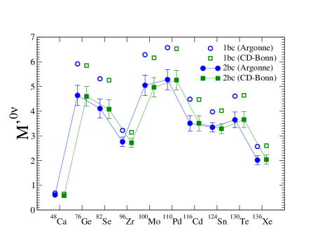
Figure 1: (Color online) Nuclear matrix elements $M^{\prime 0\nu}$ for all the nuclei considered here. The empty circles and squares represent the results with the one-body current only, and the solid circles and squares the average of the results with two-body currents included. The error bars represent the dispersion in those values (see text).

There are several reasons for the first fact. As Ref. Menéndez et al. (2011) shows, the degree of quenching decreases with increasing momentum transfer. An as we noted earlier, $2\nu\beta\beta$ decay involves almost no momentum transfer by the currents, while $0\nu\beta\beta$ decay involves momentum transfers that are typically about 100 MeV and still contribute non-negligibly at several hundred MeV. In addition, the $0\nu\beta\beta$ matrix element contains a Fermi part, for which we have assumed no quenching. While this assumption may not be completely accurate, it is implied at low momentum transfer by CVC. The overall quenching of the vector current is certain to be less than that of the axial-vector current. (In the results listed in Tables 1 and 2 the Fermi matrix elements are smaller than in some other calculations because the isovector particle-particle interaction was adjusted as explained in Ref. Šimkovic et al. (2013) to reflect isospin symmetry.)

Why is the QRPA $0\nu\beta\beta$ quenching less than that in the shell model? Part of the reason, as we noted in the introduction, is that in the QRPA the strength of the isoscalar pairing interaction, which we call $g_{pp}^{T=0}$, is adjusted to reproduce the measured $2\nu\beta\beta$ rate. The suppression of $2\nu\beta\beta$ decay by two-body currents implies that the value of $g_{pp}^{T=0}$ is smaller than it would be without those currents. The smaller $g_{pp}^{T=0}$ in turn implies less quenching for the $0\nu\beta\beta$ matrix element.

Figure 2 illustrates this idea. The upper panel shows the $2\nu\beta\beta$ matrix element, with (solid red) and without (dashed blue) two-body currents. The two vertical lines indicate the values of $g_{pp}^{T=0}$ needed to reproduce the “measured” matrix element Agostini et al. (2013), defined as that which gives the lifetime under the assumption that $g_{A}$ is unquenched. The value of $g_{pp}^{T=0}$ that works with the two-body currents is smaller. The lower panel shows the consequences for $0\nu\beta\beta$ decay. The longer (purple) arrow represents the quenching that would obtain if $g_{pp}^{T=0}$ were not adjusted for the presence of the two-body currents (as is the case in the shell model, where the interaction is fixed ahead of time). The shorter arrow represents the same quenching after adjusting $g_{pp}^{T=0}$. The requirement that we reproduce $2\nu\beta\beta$ decay thus means that the $0\nu\beta\beta$ matrix element is quenched noticeably less than it would otherwise be.

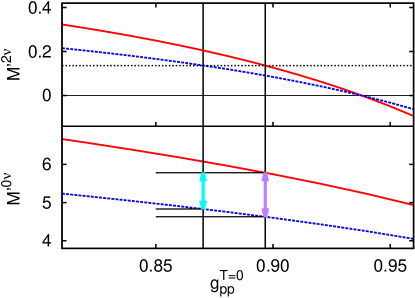
Figure 2: (Color online) The quenching of $2\nu\beta\beta$ and $0\nu\beta\beta$ decay by two-body currents in $\chi$EFT. Top: $M^{\prime 2\nu}$ vs. the $g_{pp}^{T=0}$, the strength of isoscalar pairing. The solid (red) line is the unquenched matrix element and the dashed (blue) line the matrix element with quenching caused by two-body currents, with the parameterization EGM+$\delta c_{i}$ from Ref. Menéndez et al. (2011). The dotted black line is the measured matrix element Agostini et al. (2013) under the assumption that $g_{A}$ is unquenched. The vertical lines are the values of $g_{pp}^{T=0}$ that reproduce the measurement with and without two-body currents. Bottom: The same, for $M^{\prime 0\nu}$ (without a measured value). The long (purple) arrow represents the quenching when $g_{pp}^{T=0}$ is not readjusted to reproduce $2\nu\beta\beta$ decay. The short (cyan) arrow is the quenching when $g_{pp}^{T=0}$ is readjusted.

Another difference between the QRPA and the shell model is that the QRPA works in a much larger single-particle space (at the price of working with only a particular kind of correlation). This larger space presumably means larger contributions at high momentum transfer. Since the quenching decreases with momentum transfer, the contributions of the high-angular-momentum multipoles are less affected by the two-body currents than their low-angular-momentum counterparts. The large QRPA model space therefore suggests that the quenching of $0\nu\beta\beta$ decay is less than it would be in a shell model calculation. The size of this effect, however, is hard to quantify.

IV Discussion

It is clear, in today’s terminology, that some of the quenching of spin operators in nuclei is due to the use of restricted model spaces and some to many-body currents. Model-space truncation can exclude strength that may be pushed to high energies, and the omission of two-body currents leaves delta-hole excitations, among other things, unaccounted for. The question of which effect is more important is still open. If two-body currents are behind most of the quenching, as recent fits of the $c$ parameters seem to suggest, then $2\nu\beta\beta$ decay is very likely more quenched than $0\nu\beta\beta$ decay and existing calculations of $0\nu\beta\beta$ decay that don’t include quenching are at least in the right ballpark. We’ve seen, under this assumption, that such is the case in the QRPA, even a bit more than in the shell model.

It is still possible, as older meson-exchange models suggest Towner (1987), that the effects of many-body currents are small. In that event the quenching of neutrinoless decay would be unrelated to the two-body currents and could be similar in magnitude to the quenching of two-neutrino decay, a state of affairs that would make $0\nu\beta\beta$ experiments less sensitive to a Majorana neutrino mass than we currently believe. A strong argument that this state of affairs is real, however, has yet to be presented. It seems likely to us that the quenching of $0\nu\beta\beta$ matrix elements is around the size indicated by the $\chi$EFT-plus-QRPA analysis carried out here.