Transverse-momentum distribution and nuclear modification factor for neutral pions in the forward-rapidity region in proton-lead collisions at $\sqrt{s_{NN}}=$5.02\text{\,}\mathrm{TeV}$$

Abstract

The transverse momentum ($p_{\text{T}}$) distribution for inclusive neutral pions in the very forward rapidity region has been measured, with the Large Hadron Collider forward detector (LHCf), in proton–lead collisions at nucleon-nucleon center-of-mass energies of $\sqrt{s_{NN}}=$5.02\text{\,}\mathrm{TeV}$$ at the LHC. The $p_{\text{T}}$ spectra obtained in the rapidity range $-11.0<y_{\text{lab}}<-8.9$ and $0<p_{\text{T}}<$0.6\text{\,}\mathrm{GeV}$$ (in the detector reference frame) show a strong suppression of the production of neutral pions after taking into account ultra-peripheral collisions. This leads to a nuclear modification factor value, relative to the interpolated $p_{\text{T}}$ spectra in proton-proton collisions at $\sqrt{s}=$5.02\text{\,}\mathrm{TeV}$$, of about 0.1–0.4. This value is compared with the predictions of several hadronic interaction Monte Carlo simulations.

I Introduction

Measurements of particle production in hadronic interactions at high energies play an unique role in the study of strong interactions described by Quantum Chromodynamics (QCD). For example, as first discovered in measurements at HERA H1 ; ZEUS , it is still not well understood how a parton (dominantly gluon) density increases or even saturates when the momentum fraction that the parton itself carries is small (denoted as Bjorken-$x$). This even though the understanding of the behaviour of hadron constituents (partons) has been improving both theoretically and experimentally in the past few decades.

Such kind of phenomena at small Bjorken-$x$ are known to be more visible in events at large rapidities. Since at large rapidities partons in projectile and target hadrons generally have large and small momentum fractions respectively, Bjorken-$x$ in the target should be smaller than in mid rapidity events. Moreover, in case of nuclear target interactions, the parton density in the target nucleus is expected to be larger by $\sim A^{1/3}$. In these interactions partons in the projectile hadron would lose their energy while traveling in the dense QCD matter. Particle production mechanisms change accordingly when compared to those in nucleon-nucleon interactions.

These phenomena have been observed by several experiments at the Super Proton Synchrotron (SPS, CERN), at the Relativistic Heavy Ion Collider (RHIC, BNL), and at the Large Hadron Collider (LHC, CERN). The BRAHMS and STAR experiments at RHIC showed the modification of particle production spectra at forward rapidity BRAHMS ; STAR by comparing the $p_{\text{T}}$ spectra in deuterium–gold ($d$–Au) collisions at nucleon-nucleon center-of-mass energies $\sqrt{s_{NN}}=$200\text{\,}\mathrm{GeV}$$ with those in proton–proton ($p$–$p$) collisions at center-of-mass energies $\sqrt{s}=$200\text{\,}\mathrm{GeV}$$. Especially, a comparison of the experimental results between different rapidity regions by BRAHMS (pseudorapidity $\eta=2.2$ and 3.2) and STAR ($\eta=4.0$) indicates that particle production is strongly suppressed with increasing pseudorapidity. Also at LHC the same suppression of hadron production has been found by the ALICE and LHCb experiments, both at mid and forward rapidities ALICE ; LHCb .

Thus one could ask, in what way does particle production take place within an extremely dense QCD matter in very forward rapidity regions ? There are models that actually try to make quantitative predictions in these regions. For example under the black body assumption the meson production is found to be strongly suppressed as a result of limiting fragmentation with a broadened $p_{\text{T}}$ distribution Blackbody . A suppression of particle production is also predicted using the color glass condensate formalism because of the gluon saturation dynamics JalilianMarian ; Albacete . Similarly hadronic interaction Monte Carlo (MC) simulations covering soft-QCD show a modification of the $p_{\text{T}}$ distributions. Experimental data that confirm the theoretical and phenomenological predictions and possibly constrain the remaining degrees of freedom in such models would thus be very welcome.

Understanding of particle production in very forward rapidity regions in nuclear target interactions is also of importance for ultrahigh-energy cosmic ray interactions, where parton density is expected to be much higher than at LHC energies due to the dependance of Bjorken-$x\propto 1/\sqrt{s}$. In high energy cosmic-ray-observation, energy and chemical composition of primary cosmic rays are measured by analysing the cascade showers produced by the cosmic rays interacting with the nuclei in the earth atmosphere UHECR . Secondary particles produced in the atmospheric interaction are, of course, identical to the forward emitted particles from the hadronic interactions at equivalent collision energy. In fact current modeling of particle production in nuclear interactions is limited by the available energy at the accelerators and is the cause of large systematic uncertainties in high energy cosmic ray physics.

The Large Hadron Collider forward (LHCf) experiment LHCfTDR is designed to measure the hadronic production cross sections of neutral particles emitted in very forward angles in $p$–$p$ and proton-lead ($p$–Pb) collisions at the LHC, including zero degree. The LHCf detectors (see Sec. II) cover a pseudorapidity range larger than 8.4 and are capable of precise measurements of the forward high-energy inclusive-particle-production cross sections of photons, neutrons, and other neutral mesons and baryons. Therefore the LHCf experiment provides a unique opportunity to investigate the effects of high parton density which is the case in the small Bjorken-$x$ region and in $p$–Pb collisions at high energies.

In the analysis presented in this paper, the focus is placed on the neutral pions ($\pi^{0}$s) emitted into the direction of the proton beam (proton remnant side), the most sensitive probe to the details of the $p$–Pb interactions. From the LHCf measurements, the inclusive production rate and the nuclear modification factor for $\pi^{0}$s in the rapidity range of $-11.0<y_{\text{lab}}<-8.9$ in the detector reference frame are then derived as a function of the $\pi^{0}$ transverse momentum.

The paper is organised as follows. Sec. II gives a brief description of the LHCf detectors. Section III and Sec. IV summarize the data taking conditions and the MC simulation methodology, respectively. In Sec. V the analysis framework is described, while the factors that contribute to the systematic uncertainties are explained in Sec. VI. Finally the analysis results are presented and discussed in Sec. VII. Concluding remarks are found in Sec. VIII.

II The LHCf detector

Two independent detectors called the LHCf Arm1 and Arm2 were assembled originally to study $p$–$p$ collisions at the LHC LHCfJINST ; LHCfsilicon . In $p$–Pb collisions at $\sqrt{s_{NN}}=$5.02\text{\,}\mathrm{TeV}$$, only the LHCf Arm2 detector was used to measure the secondary particles emitted into the proton remnant side. Hereafter the LHCf Arm2 detector is denoted as the LHCf detector for brevity. The LHCf detector has two sampling and imaging calorimeters composed of 44 radiation lengths of tungsten and 16 sampling layers of $3\text{\,}\mathrm{mm}$ thick plastic scintillators. The transverse sizes of the calorimeters are 25$\times$$25\text{\,}\mathrm{mm}$² and 32$\times$$32\text{\,}\mathrm{mm}$². Four X-Y layers of silicon microstrip sensors are interleaved with the layers of tungsten and scintillator in order to provide the transverse profiles of the showers. Readout pitches of the silicon microstrip sensors are $0.16\text{\,}\mathrm{mm}$ LHCfsilicon .

The LHCf detector was installed in the instrumentation slot of the target neutral absorber (TAN) TAN located $140\text{\,}\mathrm{m}$ in the direction of the ALICE interaction point (IP2) from the ATLAS interaction point (IP1) and at a zero-degree collision angle. The trajectories of charged particles produced at IP1 and directed towards the TAN are bent by the inner beam separation dipole magnet D1 before reaching the TAN itself. Consequently, only neutral particles produced at IP1 enter the LHCf detector. The vertical position of the LHCf detector in the TAN is manipulated so that the LHCf detector covers the pseudorapidity range from 8.4 to infinity for a beam crossing angle of $145\text{\,}\mathrm{\SIUnitSymbolMicro rad}$, especially the smaller calorimeter covers the zero-degree collision angle. After the operations in $p$–Pb collisions, the LHCf detector was uninstalled from the instrumentation slot of the TAN on April, 2013.

More details on the scientific goals of the experiment are given in Ref. LHCfTDR . The construction of the LHCf detectors (Arm1 and Arm2) is reported in Refs. LHCfJINST ; LHCfsilicon and the performance of the detectors has been studied in the previous reports SPS2007 ; LHCfIJMPA .

III Experimental data taking conditions

The experimental data used for the analysis in this paper were obtained in $p$–Pb collisions at $\sqrt{s_{NN}}=$5.02\text{\,}\mathrm{TeV}$$ with a $145\text{\,}\mathrm{\SIUnitSymbolMicro rad}$ beam crossing angle. The beam energies were $4\text{\,}\mathrm{TeV}$ for protons and $1.58\text{\,}\mathrm{TeV}$ per nucleon for Pb nuclei. Since the beam energies were asymmetric the nucleon-nucleon center-of-mass in $p$–Pb collisions shifted to rapidity = $-0.465$, with the proton beam traveling at $\theta=\pi$ and the Pb beam at $\theta=0$.

Data used in this analysis were taken in three different runs. The first (LHC Fill 3478) was taken on January 21, 2013 from 02:14 to 03:53. The second and third runs (LHC Fill 3481) were taken on January 21, 2013 from 21:03 to 23:36 and January 22, 2013 from 03:47 to 04:48, respectively. The integrated luminosity of the data was $0.63\text{\,}\mathrm{n}\mathrm{b}^{-1}$ after correcting for the live time of data acquisition systems CERNLumi . The average live time percentages for LHC Fill 3478 and 3481 were $12.1\text{\,}\mathrm{\char 37\relax}$ and $6.3\text{\,}\mathrm{\char 37\relax}$ respectively, the smaller live time percentage in Fill 3481 relative to Fill 3478 being due to a difference in the instantaneous luminosities. These three runs were taken with the same data acquisition configuration. In all runs the trigger scheme was essentially identical to that used in $p$–$p$ collisions at $\sqrt{s}=$7\text{\,}\mathrm{TeV}$$. The trigger efficiency was greater than $99\text{\,}\mathrm{\char 37\relax}$ for photons with energies $E>$100\text{\,}\mathrm{GeV}$$ LHCfIJMPA .

The multihit events that have more than one shower event in a single calorimeter may appear due to pileup interactions in the same bunch crossing and then could potentially cause a bias in the $p_{\text{T}}$ spectra. However, considering the acceptance of the LHCf detector for inelastic collisions $\sim 0.035$, the multihit probability due to the effects of pileup is estimated only $0.4\text{\,}\mathrm{\char 37\relax}$ and is therefore producing a negligible effect. Detailed discussions of pileup effects and background events from collisions between the beam and residual gas molecules in the beam tube can be found in previous reports LHCfIJMPA ; LHCfphoton .

Also beam divergence can cause a smeared beam spot at the TAN leading to a bias in the measured $p_{\text{T}}$ spectra. The beam divergence at IP1 was $\varepsilon/\beta^{\ast}=$32\text{\,}\mathrm{\SIUnitSymbolMicro rad}$$ Jowett for the three fills mentioned, corresponding to a beam spot size at the TAN of roughly $\sigma_{\text{TAN}}=$4.5\text{\,}\mathrm{mm}$$. The effect of a non-zero beam spot size at the TAN is evaluated by comparing two $p_{\text{T}}$ spectra predicted by toy MC simulations; one assuming a beam spot size of zero and another assuming that the beam axis positions fluctuates following a Gaussian distribution with $\sigma_{\text{TAN}}=$4.5\text{\,}\mathrm{mm}$$. The $\pi^{0}$ yield at $p_{\text{T}}=$0.6\text{\,}\mathrm{GeV}$$ is found to increase by a factor 1.8 at most. This effect is taken into account in the final results to the $p_{\text{T}}$ spectra.

IV Monte Carlo simulations methodology

MC simulations were performed in two steps:
(I) $p$–Pb interaction event generation at IP1 explained in Sec. IV.1 and (II) particle transport from IP1 to the LHCf detector and consequent simulation of the response of the LHCf detector (Sec. IV.2).

MC simulations which were then used for the validation of reconstruction algorithms and cut criteria, and the estimation of systematic uncertainties follow steps (I) and (II). These MC simulations are denoted as reference MC simulations. On the other hand, MC simulations used only for comparisons with measurement results in Sec. VII are limited to step (I) only, since the final $p_{\text{T}}$ spectra in Sec. VII are already corrected for detector responses and eventual reconstruction bias.

IV.1 Signal modeling

Whenever the impact parameter of proton and Pb is smaller than the radius of each particle, soft-QCD induced events are produced. These $p$-Pb interactions at $\sqrt{s_{NN}}=$5.02\text{\,}\mathrm{TeV}$$ and the resulting flux of secondary particles emitted into forward rapidity region with their kinematics are simulated using various hadronic interaction models (dpmjet 3.04 DPM3 , qgsjet II-03 QGS2 , and epos 1.99 EPOS ). Dpmjet 3.04 also takes into account the Fermi motion of the nucleons in Pb nucleus and the Cronin effect Cronin . Fermi motion enhances the $\pi^{0}$ yields at most by $5\text{\,}\mathrm{\char 37\relax}$ in the LHCf $p_{\text{T}}$ covered range $p_{\text{T}}<$0.6\text{\,}\mathrm{GeV}$$, while the Cronin effect is not significant in this $p_{\text{T}}$ range.

On the other hand, when the impact parameter is larger than the overlapping radii of each particle, so-called ultra-peripheral collisions (UPCs) can occur. In UPCs virtual photons are emitted by the relativistic Pb nucleus which can then collide with the proton beam UPC . The energy spectrum of these virtual photons follows the Weizsäcker-Williams approximation WW . The sophia SOPHIA MC generator is used to simulate the photon–proton interaction in the rest frame of the proton and then the secondary particles generated by sophia are boosted along the proton beam. For heavy nuclei with the radius $R_{\text{A}}$, the virtuality of the photon $|q^{2}|<(\hslash c/R_{\text{A}})^{2}$ can be neglected and the photons are regarded as real photon in the simulation in this analysis.

In these MC simulations, $\pi^{0}$s from short-lived particles that decay within $1\text{\,}\mathrm{m}$ from IP1, mostly $\eta$ mesons decaying into $3\pi^{0}$ ($\lesssim$10\text{\,}\mathrm{\char 37\relax}$$ relative to all $\pi^{0}$s), are also accounted for consistently with the treatment of the experimental data.

IV.2 Simulation of particle transport from IP1 to the LHCf detector and of the detector response

The generated secondary particles are transported in the beam pipe from IP1 to the TAN, taking into account the bending of charged particles’ trajectory by the Q1 quadrupole and the D1 beam separation dipole, particle decays, and particle interactions with the beam pipe wall and the Y-shaped beam-vacuum-transition chamber made of copper.

Finally the showers produced in the LHCf detector by the particles arriving at the TAN and the detector response are simulated with the cosmos and epics libraries EPICS . The detector position survey data and random fluctuations due to electrical noise are taken into account. The simulations of the LHCf detector are tuned to the test beam data taken at SPS, CERN in 2007 and 2012 SPS2007 ; SPSneutron .

V Analysis framework

V.1 $\pi^{0}$ event reconstruction and selection

Since $\pi^{0}$s decay into two photons very close to their point of creation at IP1, each photon’s direction is geometrically calculated using the impact coordinates at the LHCf detector and the distance between IP1 and the detector itself. Photon four-momentum is then derived by combining the photon’s energy as measured by the calorimeter with the previously obtained angle of emission. Candidate $\pi^{0}$s are selected from events where the invariant mass of the two photons detected is within a narrow window around the $\pi^{0}$ rest mass.

The $\pi^{0}$ events are then classified in two categories: single-hit $\pi^{0}$ and multihit $\pi^{0}$ events. The former is defined as having a single photon in each of the two calorimeter towers only, while a multihit $\pi^{0}$ event is defined as a single $\pi^{0}$ accompanied by at least one additional background particle (usually a photon or a neutron) in one of the two calorimeters. In the analysis presented here, events having two particles within the same calorimeter tower (multihit events) are rejected when the energy deposit of the background particle is above a certain threshold LHCfpi0 . Mostly then, only single-hit $\pi^{0}$ events are considered in this analysis. The final inclusive production rates reported at the end are corrected for this cut as described in Sec. V.3.

Given the geometrical acceptance of the LHCf detector and to ensure a good event reconstruction efficiency, the rapidity and $p_{\text{T}}$ range of the $\pi^{0}$s are limited to $-11.0<y_{\text{lab}}<-8.9$ and $p_{\text{T}}<$0.6\text{\,}\mathrm{GeV}$$, respectively. The reconstructed invariant mass of the reference MC simulations peaks at $134.8\pm$0.2\text{\,}\mathrm{MeV}$$ and reproduces well the measured data which peaks at $134.7\pm$0.1\text{\,}\mathrm{MeV}$$, reproducing the $\pi^{0}$ mass. The uncertainties given for the mass peaks are statistical only.

Standard reconstruction algorithms used for this analysis are described in Ref. LHCfpi0 ; LHCfIJMPA and the $\pi^{0}$ event selection criteria that are applied prior to the reconstruction of the $\pi^{0}$ kinematics are summarized in Tab. 1. Systematic uncertainties are discussed in Sec. VI.

Table 1: Summary of the criteria for the selection of the $\pi^{0}$ sample.

Incident position	within $2\text{\,}\mathrm{mm}$ from the edge of calorimeter
Energy threshold	$E_{\text{photon}}>$100\text{\,}\mathrm{GeV}$$
Number of hits	Single-hit in each calorimeter
PID	Photon like in each calorimeter

V.2 Background subtraction

Background contamination of the $\pi^{0}$ events from hadronic events and the causal coincidence of two photons not originated from the decay of a single $\pi^{0}$ are taken into account by subtracting the relevant contribution using a sideband method LHCfpi0 .

Figure 1 shows the reconstructed two-photon invariant mass distribution of the experimental data in the rapidity range $-9.4<y_{\text{lab}}<-9.2$. The sharp peak around $135\text{\,}\mathrm{MeV}$ is owing to $\pi^{0}$ events. The solid curve indicates the best fit of a composite physics model to the invariant mass distribution of the data; an asymmetric Gaussian distribution for the signal component and a third order Chebyshev polynomial function for the background component (dashed curve). The signal window is defined as the invariant mass region within the two solid arrows shown in Fig. 1, where the lower and upper limits are given by $\hat{m}-3\sigma_{l}$ and $\hat{m}+3\sigma_{u}$, respectively. $\hat{m}$ denotes the expected mean, and $\sigma_{l}$ and $\sigma_{u}$ denote 1 $\sigma$ deviations for lower and upper side of the signal component, respectively. The signal-rich rapidity–$p_{\text{T}}$ distributions are obtained by the events contained inside of the signal window. The remaining contribution of background events in the signal window is eliminated using the rapidity–$p_{\text{T}}$ distributions obtained from the background window, constructed from the two sideband regions, [$\hat{m}-6\sigma_{l}$, $\hat{m}-3\sigma_{l}$] and [$\hat{m}+3\sigma_{u}$, $\hat{m}+6\sigma_{u}$], that are defined as the invariant mass regions within the dashed arrows in Fig. 1.

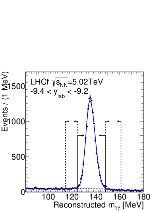
Figure 1: (color online). Reconstructed invariant mass distribution within the rapidity range from $-9.4$ to $-9.2$. The solid curve shows the best-fit composite physics model to the invariant mass distribution. The dashed curve indicates the background component. Solid and dashed lines indicate the signal and background windows, respectively.

V.3 Corrections to the $p_{\text{T}}$ spectra

The raw rapidity–$p_{\text{T}}$ distributions must be corrected for (1) the reconstruction inefficiency and the smearing caused by finite position and energy resolutions, (2) geometrical acceptance and branching ratio of $\pi^{0}$ decay, and (3) the loss due to multihit $\pi^{0}$.

First, an iterative Bayesian method Dagostini is used to simultaneously correct for both the reconstruction inefficiency and the smearing. The unfolding procedure for the data is found in paper LHCfpi0 .

Next, a correction for the limited aperture of the LHCf calorimeters must be applied. The correction is derived from the rapidity–$p_{\text{T}}$ phase space. The determination of the correction coefficients follow the same method used in the $\pi^{0}$ event analysis in $p$–$p$ collisions at $\sqrt{s}=$7\text{\,}\mathrm{TeV}$$ LHCfpi0 .

Finally, the loss of multihit $\pi^{0}$ events, briefly mentioned in Sec. V.1, is corrected for using the MC event generators. A range of ratios of multihit plus single-hit to single-hit $\pi^{0}$ events is estimated using three different hadronic interaction models (dpmjet 3.04, qgsjet II-03, and epos 1.99) for each rapidity and $p_{\text{T}}$ range. The observed $p_{\text{T}}$ spectra are then multiplied by the average of these ratios and the contribution to the systematic uncertainty is derived from the observed variations among the interaction models. The estimated range of the flux of multihit $\pi^{0}$ events lies within a range $0\text{\,}\mathrm{\char 37\relax}$–$10\text{\,}\mathrm{\char 37\relax}$ of the flux of single-hit $\pi^{0}$ events. The single-hit $\pi^{0}$ spectra are then corrected to represent the inclusive $\pi^{0}$ production spectra.

All the procedures were verified using the reference MC simulations mentioned in Sec. IV.

VI Systematic uncertainties

We follow the same approach to estimate the systematic uncertainties as in Ref. LHCfpi0 . Since systematic uncertainties on particle identification, single-hit selection, and position-dependent corrections for both shower leakage and light yield of the calorimeter are independent of the beam energy and type, the systematic errors are taken directly from Ref. LHCfpi0 .

Other terms deriving from the energy scale, beam axis offset, and luminosity are updated consistently to the current understanding of the LHCf detector and the beam configuration in $p$–Pb collisions. These terms are discussed in the following subsections. Table 2 summarises the systematic uncertainties for the analysis.

VI.1 Energy scale

The uncertainty on the measured photon energy was investigated in the beam test at SPS SPS2007 and also by performing a calibration with a radioactive source LHCfJINST . The estimated uncertainty on the photon energy from these tests is valued at $3.5\text{\,}\mathrm{\char 37\relax}$. This uncertainty is dominated by the conversion factors that relate measured charge to deposited energy SPS2007 and in fact, the reconstructed invariant mass of two photons reproduces the $\pi^{0}$ rest mass within the uncertainty of $3.5\text{\,}\mathrm{\char 37\relax}$ as shown in Fig. 1.

The systematic shift of bin contents due to energy scale uncertainties is estimated using two different $p_{\text{T}}$ spectra in which the photon energy is artificially scaled to the two extremes ($\pm$3.5\text{\,}\mathrm{\char 37\relax}$$). The ratios of the two extreme spectra to the non-scaled spectrum are assigned as systematic shifts of bin contents for each bin.

VI.2 Beam axis offset

The projected position of the proton beam axis on the LHCf detector (beam centre) varies from Fill to Fill owing to the beam configuration, beam transverse position and crossing angles, at IP1. The beam centre on the LHCf detector can be determined by two methods; first we use the distribution of incident particle positions as measured by the LHCf detector and second we also use the information from the beam position monitors (BPMSW) installed $\pm$21\text{\,}\mathrm{m}$$ from IP1 BPM .

From analysis results in $p$–$p$ collisions at $\sqrt{s}=$7\text{\,}\mathrm{TeV}$$, the beam centre positions obtained by the two methods applied to LHC Fills 1089–1134 were found to be consistent within $1\text{\,}\mathrm{mm}$. The systematic shifts to the $p_{\text{T}}$ spectra are then evaluated by taking the ratio of spectra with the beam centre displaced by $\pm$1\text{\,}\mathrm{mm}$$ to spectra with no displacement present. The fluctuations of the beam centre position modify the $p_{\text{T}}$ spectra by $5\text{\,}\mathrm{\char 37\relax}$–$20\text{\,}\mathrm{\char 37\relax}$ depending on the rapidity range.

VI.3 Luminosity

The luminosity value used for the analysis is derived from on the online information provided by the ATLAS experiment. Since there is currently no robust estimation on the luminosity error by the ATLAS experiment, we assign a conservative $\pm$20\text{\,}\mathrm{\char 37\relax}$$ to the uncertainty. A more precise estimation of the luminosity will be reported in future by the ATLAS collaboration.

Table 2: Summary of the systematic uncertainties. Numerical values indicate the maximum variation of bin contents in the $p_{\text{T}}$ spectra.

Energy scale	$5\text{\,}\mathrm{\char 37\relax}$–$20\text{\,}\mathrm{\char 37\relax}$
Particle identification	$0\text{\,}\mathrm{\char 37\relax}$–$20\text{\,}\mathrm{\char 37\relax}$
Offset of beam axis	$5\text{\,}\mathrm{\char 37\relax}$–$20\text{\,}\mathrm{\char 37\relax}$
Single-hit selection	$3\text{\,}\mathrm{\char 37\relax}$
Position-dependent correction	$5\text{\,}\mathrm{\char 37\relax}$–$30\text{\,}\mathrm{\char 37\relax}$
Luminosity	$20\text{\,}\mathrm{\char 37\relax}$

VII Results and discussion

VII.1 The QCD induced transverse momentum distribution

The $p_{\text{T}}$ spectra obtained from the data analysed are presented in Fig. 2. The spectra are categorized into six ranges of rapidity $y_{\text{lab}}$: [-9.0, -8.9], [-9.2, -9.0], [-9.4, -9.2], [-9.6, -9.4], [-10.0, -9.6], and [-11.0, -10.0]. The spectra have all the corrections discussed in Sec. V.3 applied. The inclusive $\pi^{0}$ production rate is given as

$$\frac{1}{\sigma^{\text{pPb}}_{\text{inel}}}E\frac{d^{3}\sigma^{\text{pPb}}}{dp^{3}}=\frac{1}{N^{\text{pPb}}_{\text{inel}}}\frac{d^{2}N^{\text{pPb}}(p_{\text{T}},y)}{2\pi p_{\text{T}}dp_{\text{T}}dy}.$$ (1)

where $\sigma^{\text{pPb}}_{\text{inel}}$ is the inelastic cross section for $p$–Pb collisions at $\sqrt{s_{NN}}=$5.02\text{\,}\mathrm{TeV}$$ and $Ed^{3}\sigma^{\text{pPb}}/dp^{3}$ is the inclusive cross section of $\pi^{0}$ production. The number of inelastic $p$–Pb collisions, $N^{\text{pPb}}_{\text{inel}}$, used for normalizing the production rates of Fig. 2 is calculated from $N^{\text{pPb}}_{\text{inel}}$ = $\sigma^{\text{pPb}}_{\text{inel}}\int{\cal L}dt$, assuming an inelastic $p$–Pb cross section $\sigma^{\text{pPb}}_{\text{inel}}=$2.11\text{\,}\mathrm{b}$$. The value for $\sigma^{\text{pPb}}_{\text{inel}}$ is derived from the inelastic $p$–$p$ cross section $\sigma^{\text{pp}}_{\text{inel}}$ and the Glauber multiple collision model Glauber ; dEnterria . Using the integrated luminosities shown in Sec. III, $N^{\text{pPb}}_{\text{inel}}$ is 9.33$\times$10⁷. $d^{2}N^{\text{pPb}}(p_{\text{T}},y)$ is the number of $\pi^{0}$s detected in the transverse momentum interval ($dp_{\text{T}}$) and the rapidity interval ($dy$) with all corrections applied.

In Fig. 2, the filled circles represent the data from the LHCf experiment. The error bars and shaded rectangles indicate the 1 standard deviation statistical and total systematic uncertainties respectively. The total systematic uncertainties are given by adding all uncertainty terms except the one for luminosity in quadrature. The vertical dashed lines shown for the rapidity ranges greater than $-9.2$ indicate the $p_{\text{T}}$ threshold of the LHCf detector due to the photon energy threshold and the geometrical acceptance of the detector. The contribution from UPCs is presented as open squares (normalized to $1/2$ for visibility). This UPC contribution is estimated with the MC simulations introduced in Sec. IV.1 using the UPC cross section from LHCfUPC .

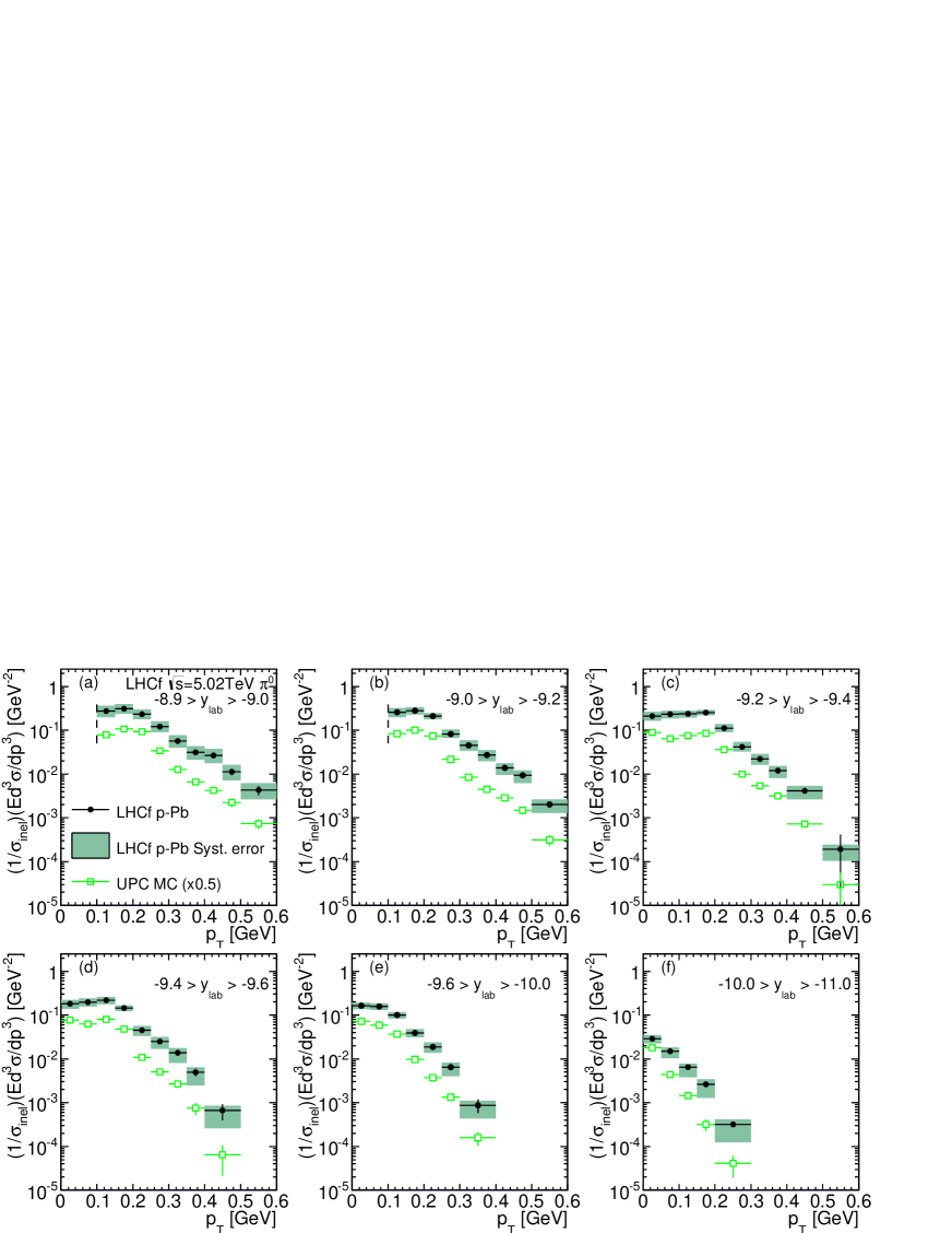
Figure 2: (color online). Experimental $p_{\text{T}}$ spectra of the LHCf detector (filled circles). Error bars and shaded rectangles indicate the statistical and systematic uncertainties respectively. The open squares indicate the estimated contribution from UPCs.

To obtain the soft-QCD component, the UPC contribution must be subtracted from the measured $p_{\text{T}}$ spectra. This is achieved by simply subtracting, point by point, the UPC induced $p_{\text{T}}$ spectra (open squares in Fig. 2) from the total $p_{\text{T}}$ spectra (filled circles in Fig. 2). Uncertainties in the subtracted results are obtained by adding the statistical and systematic errors in quadrature. The theoretical uncertainty on the UPC estimation $\pm$5\text{\,}\mathrm{\char 37\relax}$$ derives mainly from the knowledge of the virtual photon flux given by the relativistic Pb nucleus and of the virtual photon-proton cross section LHCfUPC . The inclusive production rates of $\pi^{0}$s measured by LHCf after the subtraction of the UPC component are summarized in Appendix A.

Figure 3 shows the LHCf data $p_{\text{T}}$ spectra after subtraction of the UPC component (filled circles). The size of the error bars correspond to $68\text{\,}\mathrm{\char 37\relax}$ confidence intervals (including both statistical and systematic uncertainties). The $p_{\text{T}}$ spectra in $p$–Pb collisions at $5.02\text{\,}\mathrm{TeV}$ predicted by the hadronic interaction models, dpmjet 3.04 (solid line, red), qgsjet II-03 (dashed line, blue), and epos 1.99 (dotted line, magenta), are also shown in the same figure for comparison. Predictions by the three hadronic interaction models do not include the UPC component. The experimental $p_{\text{T}}$ spectra are corrected for detector response, event selection and geometrical acceptance efficiencies, so that the $p_{\text{T}}$ spectra of the interaction models can be compared directly to the experimental spectra.

In Fig. 3, among the predictions given by the hadronic interaction models tested here, dpmjet 3.04 and epos 1.99 show a good overall agreement with the LHCf measurements. However qgsjet II-03 predicts softer $p_{\text{T}}$ spectra than the LHCf measurements and the other two hadronic interaction models. Similar features of these hadronic interaction models are also seen in $p$–$p$ collisions at $\sqrt{s}=$7\text{\,}\mathrm{TeV}$$ LHCfpi0 .

In Fig. 3, the $p_{\text{T}}$ spectra in $p$–$p$ collisions at $\sqrt{s}=$5.02\text{\,}\mathrm{TeV}$$ are also added and will be useful for the derivation of the nuclear modification factor described later in Sec. VII.3. These spectra are multiplied by a factor 5 for visibility. The derivation of the $p_{\text{T}}$ spectra in $p$–$p$ collisions at $\sqrt{s}=$5.02\text{\,}\mathrm{TeV}$$ is explained in detail in Appendix B.

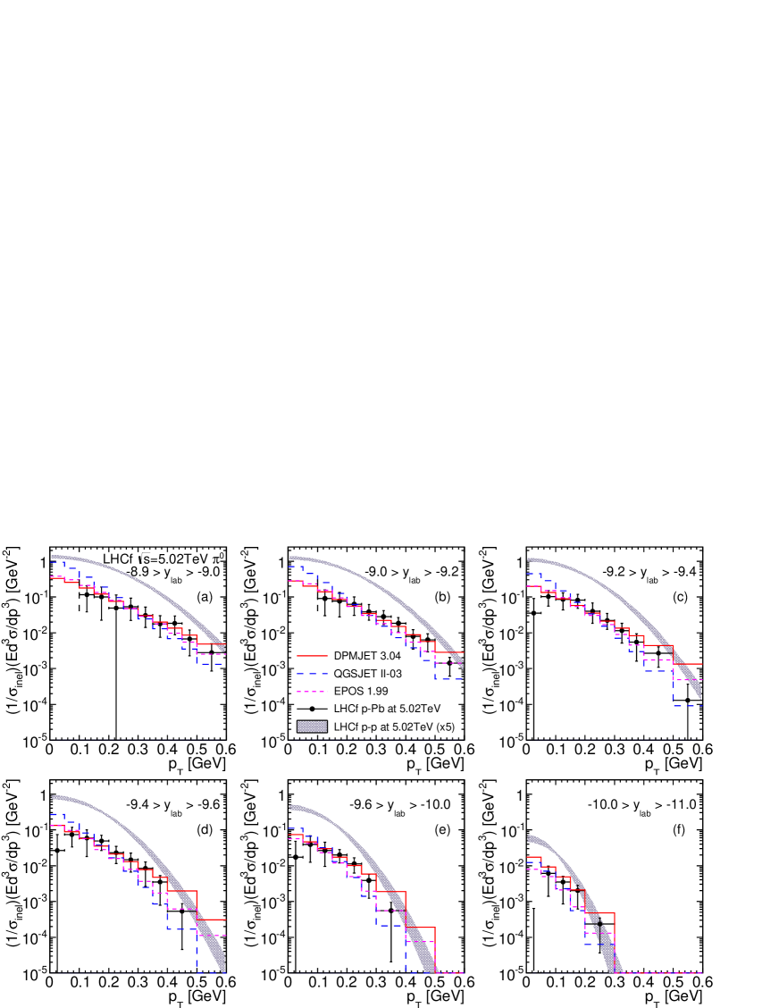
Figure 3: (color online). Experimental $p_{\text{T}}$ spectra measured by LHCf after the subtraction of the UPC component (filled circles). Error bars indicate the total uncertainties incorporating both statistical and systematic uncertainties. Hadronic interaction models predictions and derived spectra for $p$–$p$ collisions at $5.02\text{\,}\mathrm{TeV}$ are also shown (see text for details).

VII.2 Average transverse momentum.

The average transverse momentum, $\langle p_{\text{T}}\rangle$, can be obtained by fitting an empirical function to the $p_{\text{T}}$ spectra in Fig. 3 for each rapidity range. Two distributions to parametrize the $p_{\text{T}}$ spectra were chosen among the several proposed in literature: an exponential and a Gaussian. Detailed descriptions of the parametrization and derivation of $\langle p_{\text{T}}\rangle$ can be found in Ref. LHCfpi0 .

For example, the upper panel in Fig. 4 shows the experimental $p_{\text{T}}$ spectra (filled circles) and the best fit with the exponential (dashed curve, blue) and with the Gaussian distribution (dotted curve, red) in the rapidity range $-9.2>y_{\text{lab}}>-9.4$. The bottom panel in Fig. 4 shows best-fit ratio to the experimental data; exponential (blue open triangles) and Gaussian distributions (red open circles). Error bars indicate the statistical and systematic uncertainties in the both panels.

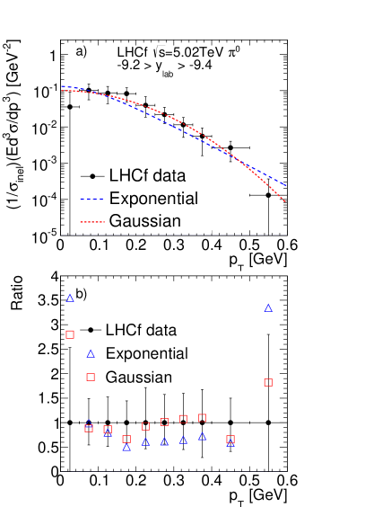
Figure 4: (color online). (a) Upper: experimental $p_{\text{T}}$ spectra (filled circles and error bars), the best-fit exponential (dashed curve) and Gaussian distributions (dotted curve). (b) Bottom: ratios of the best-fit exponential or Gaussian distribution to the experimental data (open triangles or open boxes) with statistical and systematic uncertainties (filled circles and error bars.)

On the other hand, $\langle p_{\text{T}}\rangle$ can be simply estimated by numerically integrating the $p_{\text{T}}$ spectra in Fig. 3. In this approach, $\langle p_{\text{T}}\rangle$ is obtained over the rapidity range $-9.2>y_{\text{lab}}>-10.0$ where the $p_{\text{T}}$ spectra are available down to $0\text{\,}\mathrm{GeV}$. The data in the rapidity range $-10.0>y_{\text{lab}}>-11.0$ is not used here, since the bin content in $$0\text{\,}\mathrm{GeV}$<p_{\text{T}}<$0.05\text{\,}\mathrm{GeV}$$ is negative due to the subtraction of UPCs. Although the interval for the numerical integration is bounded from above by $p_{\text{T}}^{\text{upper}}$, the high $p_{\text{T}}$ tail contribution to $\langle p_{\text{T}}\rangle$ is negligibly small.

The values of $\langle p_{\text{T}}\rangle$ obtained by the three methods are in good agreement within the uncertainties. The specific values of $\langle p_{\text{T}}\rangle$ for this paper, $\langle p_{\text{T}}\rangle_{\text{LHCf}}$, are defined as follows. For the rapidity range $-9.2>y_{\text{lab}}>-10.0$, the values of $\langle p_{\text{T}}\rangle_{\text{LHCf}}$ are taken from the weighted average of $\langle p_{\text{T}}\rangle$ from the exponential fit, the Gaussian fit, and the numerical integration. The uncertainty related to a possible bias of the $\langle p_{\text{T}}\rangle$ extraction methods is derived from the largest value among the three methods. For the other rapidity ranges to where the numerical integration is not applicable, the weighted mean and the uncertainty are obtained following the same method above but using only the exponential and the Gaussian fit. Best-fit results for the three approaches mentioned above and the values of $\langle p_{\text{T}}\rangle_{\text{LHCf}}$ are summarised in Table 3.

Figure 5 shows the $\langle p_{\text{T}}\rangle_{\text{LHCf}}$ and the predictions by hadronic interaction models as a function of the rapidity $y_{\text{lab}}$. The average $p_{\text{T}}$ of the hadronic interaction models is calculated by numerical integration. dpmjet 3.04 reproduces quite well the LHCf measurements $\langle p_{\text{T}}\rangle_{\text{LHCf}}$, while epos 1.99 is slightly softer than both dpmjet 3.04 and the LHCf measurements. qgsjet II-03 shows the smallest $\langle p_{\text{T}}\rangle$ among the three models and the LHCf measurements. These tendencies are also found in Fig. 3.

Table 3: The average $\pi^{0}$ transverse momenta for the rapidity range $-8.9>y_{\text{lab}}>-11.0$ estimated by the three approaches (exponential, Gaussian, and numerical integration). Combined results using the three approaches are denoted as LHCf results.

	Exponential fit			Gaussian fit			Numerical integration			LHCf analysis
Rapidity	$\chi^{2}$ (dof)	$\langle p_{\text{T}}\rangle$	Stat. error	$\chi^{2}$ (dof)	$\langle p_{\text{T}}\rangle$	Stat. error	$p_{\text{T}}^{\text{upper}}$	$\langle p_{\text{T}}\rangle$	Stat. error	$\langle p_{\text{T}}\rangle_{\text{LHCf}}$	Syst. error
		[MeV]	[MeV]		[MeV]	[MeV]	[GeV]	[MeV]	[MeV]	[MeV]	[MeV]
$[$-8.9, -9.0$]$	0.9 (7)	249.1	36.8	0.8 (7)	258.5	27.9				255.3	36.8
$[$-9.0, -9.2$]$	2.0 (7)	221.1	20.4	0.5 (7)	239.5	16.6				232.3	20.4
$[$-9.2, -9.4$]$	7.6 (8)	188.7	13.4	2.7 (8)	196.4	8.6	0.6	193.3	13.2	194.4	13.4
$[$-9.4, -9.6$]$	4.8 (6)	181.8	16.3	1.6 (6)	187.0	12.7	0.5	184.6	14.9	185.7	16.3
$[$-9.6, -10.0$]$	3.7 (5)	153.0	16.3	1.5 (5)	153.7	12.3	0.4	152.2	13.9	153.9	16.3
$[$-10.0,-11.0$]$	<0.1 (2)	115.1	22.2	<0.1 (2)	117.5	17.5				116.6	22.2

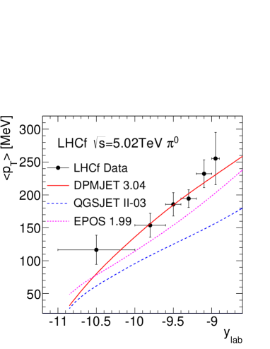
Figure 5: (color online). Average $p_{\text{T}}$ as a function of rapidity $y_{\text{lab}}$. Filled circles indicate the LHCf data. The predictions of hadronic interaction models are shown (solid curve dpmjet 3.04, dashed curve qgsjet II-03, and dotted curve epos 1.99).

VII.3 Nuclear modification factor

Finally the nuclear modification factor $R_{\textrm{pPb}}$ is derived. This factor quantifies the $p_{\text{T}}$ spectra modification caused by nuclear effects in $p$–Pb collisions. The nuclear modification factor is defined as

$$R_{\textrm{pPb}}\equiv\frac{\sigma^{\textrm{pp}}_{\textrm{inel}}}{\langle N_{\textrm{coll}}\rangle\sigma^{\textrm{pPb}}_{\textrm{inel}}}\frac{Ed^{3}\sigma^{\textrm{pPb}}/dp^{3}}{Ed^{3}\sigma^{\textrm{pp}}/dp^{3}},$$ (2)

where $Ed^{3}\sigma^{\text{pPb}}/dp^{3}$ and $Ed^{3}\sigma^{\text{pp}}/dp^{3}$ are the inclusive cross sections of $\pi^{0}$ production in $p$–Pb and $p$–$p$ collisions at $5.02\text{\,}\mathrm{TeV}$ respectively. The UPC component is already subtracted in $\sigma^{\text{pPb}}$. The uncertainty on $\sigma^{\text{pPb}}_{\text{inel}}$ is estimated to be $\pm$5\text{\,}\mathrm{\char 37\relax}$$ by comparing the $\sigma^{\text{pPb}}_{\text{inel}}$ value with other calculations and experimental results presented in CMSxsec ; ALICExsec . The average number of binary nucleon–nucleon collisions in a $p$–Pb collision, $\langle N_{\textrm{coll}}\rangle=6.9$, is obtained from MC simulations using the Glauber model dEnterria . The uncertainty in $\sigma^{\textrm{pp}}_{\textrm{inel}}/\langle N_{\textrm{coll}}\rangle$ is estimated by varying the parameters in the calculation with the Glauber model ALICE ; ALICErapidity (where the cancellation of the uncertainties in $\sigma^{\textrm{pp}}_{\textrm{inel}}$ and $\langle N_{\textrm{coll}}\rangle$ is taken into account) and is of the order of $\pm$3.5\text{\,}\mathrm{\char 37\relax}$$ . Finally the quadratic sum of the uncertainties in $\sigma^{\text{pPb}}_{\text{inel}}$ and $\sigma^{\textrm{pp}}_{\textrm{inel}}/\langle N_{\textrm{coll}}\rangle$ is added to $R_{\textrm{pPb}}$.

Since there is no data at $\sqrt{s}=$5.02\text{\,}\mathrm{TeV}$$ for $p$–$p$ collisions $Ed^{3}\sigma^{\text{pp}}/dp^{3}$ is derived by scaling the $p_{\text{T}}$ spectra taken in $p$–$p$ collisions at $7\text{\,}\mathrm{TeV}$ and $2.76\text{\,}\mathrm{TeV}$. The derivation follows three steps. First (I) the $\langle p_{\text{T}}\rangle$ values at $5.02\text{\,}\mathrm{TeV}$ are estimated by interpolating the $\langle p_{\text{T}}\rangle$ values at $7\text{\,}\mathrm{TeV}$ and $2.76\text{\,}\mathrm{TeV}$, assuming that the Feynman scaling of $\langle p_{\text{T}}\rangle$ is only a function of rapidity. Then (II) the absolute normalizations of the $p_{\text{T}}$ spectra at $5.02\text{\,}\mathrm{TeV}$ are determined by applying the measured absolute normalizations at $7\text{\,}\mathrm{TeV}$ directly to those at $5.02\text{\,}\mathrm{TeV}$. Finally (III) the $p_{\text{T}}$ spectra at $5.02\text{\,}\mathrm{TeV}$ are derived assuming that the $p_{\text{T}}$ spectra follow a Gaussian distribution with width $2\langle p_{\text{T}}\rangle/\sqrt{\pi}$ (obtained in step (I)) and using the normalizations obtained in step (II). The rapidity shift $-0.465$ explained in Sec. III is also taken into account in the $p_{\text{T}}$ spectrum at $5.02\text{\,}\mathrm{TeV}$. The details of the procedure are discussed in Appendix B.

Figure 6 shows the nuclear modification factors $R_{\textrm{pPb}}$ from the LHCf measurements and the predictions by hadronic interaction models dpmjet 3.04 (red solid line), qgsjet II-03 (blue dashed line), and epos 1.99 (magenta dotted line). The LHCf measurements, although with a large uncertainty which increases with $p_{\text{T}}$ (mainly due to systematic uncertainties in $p$–Pb collisions at $5.02\text{\,}\mathrm{TeV}$), show a strong suppression with $R_{\textrm{pPb}}$ equal 0.1 at $p_{\text{T}}\approx$0.1\text{\,}\mathrm{GeV}$$ rising to 0.3 at $p_{\text{T}}\approx$0.6\text{\,}\mathrm{GeV}$$. All hadronic interaction models predict small values of $R_{\textrm{pPb}}\approx 0.1$, and they show an overall good agreement with the LHCf measurements within the uncertainty. Clearly other analyses which are more sensitive to exclusive $\pi^{0}$ signals are needed, for example diffractive dissociation, to investigate the reason for this strong suppression. However the measured $R_{\textrm{pPb}}$ dependency on $p_{\text{T}}$ and rapidity may hint to an understanding of the break down of the $\pi^{0}$ production mechanism.

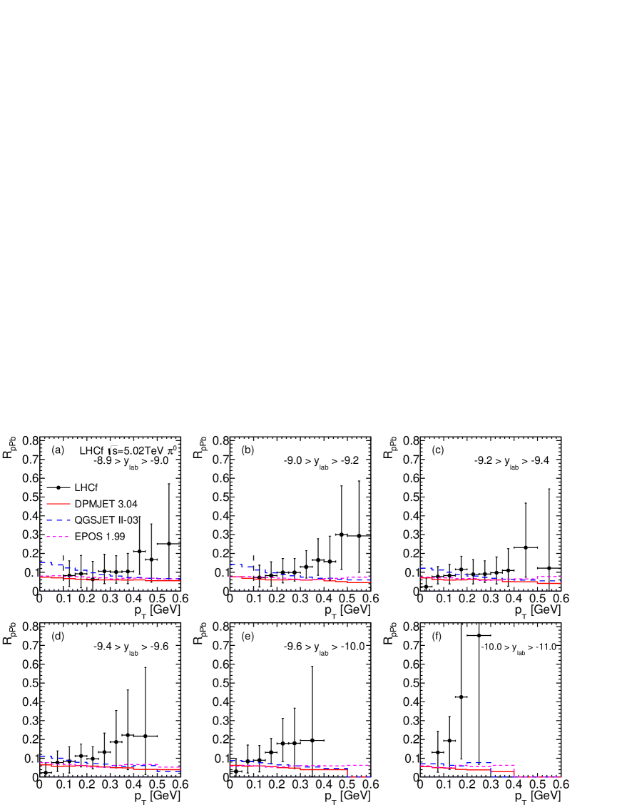
Figure 6: (color online). Nuclear modification factor for $\pi^{0}$s. Filled circles indicate the factors obtained by the LHCf measurements. Error bars indicate the total uncertainties incorporating both statistical and systematic uncertainties. Other lines are the predictions by hadronic interaction models (see text in detail.)

VIII Conclusions

The inclusive production of neutral pions in the rapidity range $-8.9>y_{\text{lab}}>-11.0$ has been measured by the LHCf experiment in $p$–Pb collisions at $\sqrt{s_{NN}}=$5.02\text{\,}\mathrm{TeV}$$ at the LHC in 2013. Transverse momentum spectra of neutral pions measured by the LHCf detectors have been compared with the predictions of several hadronic interaction models. Among the hadronic interaction models tested in this paper, dpmjet 3.04 and epos 1.99 show the best overall agreement with the LHCf data in the rapidity range $-8.9>y_{\text{lab}}>-11.0$, while qgsjet II-03 shows softer $p_{\text{T}}$ spectra relative to the the LHCf data and the other two hadronic interaction models. These tendencies are also recognized in the comparison on the average $p_{\text{T}}$ distribution as a function of rapidity $y_{\text{lab}}$.

The nuclear modification factor, $R_{\textrm{pPb}}$, derived from the LHCf measurements indicates a strong suppression of the $\pi^{0}$ production in the nuclear target relative to those in the nucleon target. All hadronic interaction models present an overall good agreement with the LHCf measurements within the uncertainty.

As a future prospect, additional analyses which are sensitive to exclusive $\pi^{0}$ spectra, are needed to reach a better understanding of this strong suppression and its break down.

Appendix A

The inclusive production rates of $\pi^{0}$s measured by LHCf after the subtraction of the UPC component are summarized in Tables 4– 9.

Table 4: Production rate for the $\pi^{0}$ production in the rapidity range $-8.9>y_{\text{lab}}>-9.0$.

$p_{\text{T}}$ range $[$GeV$]$	Production rate $[$GeV${}^{-2}]$	Syst+Stat uncertainty $[$GeV${}^{-2}]$
$[$0.10, 0.15$]$	1.17$\times 10^{-1}$	-7.83$\times 10^{-2}$, +8.91$\times 10^{-2}$
$[$0.15, 0.20$]$	1.00$\times 10^{-1}$	-7.75$\times 10^{-2}$, +8.79$\times 10^{-2}$
$[$0.20, 0.25$]$	4.90$\times 10^{-2}$	-5.57$\times 10^{-2}$, +6.43$\times 10^{-2}$
$[$0.25, 0.30$]$	5.37$\times 10^{-2}$	-3.18$\times 10^{-2}$, +3.85$\times 10^{-2}$
$[$0.30, 0.35$]$	3.09$\times 10^{-2}$	-1.69$\times 10^{-2}$, +2.11$\times 10^{-2}$
$[$0.35, 0.40$]$	1.76$\times 10^{-2}$	-1.02$\times 10^{-2}$, +1.24$\times 10^{-2}$
$[$0.40, 0.45$]$	1.82$\times 10^{-2}$	-9.42$\times 10^{-3}$, +1.12$\times 10^{-2}$
$[$0.45, 0.50$]$	6.77$\times 10^{-3}$	-4.49$\times 10^{-3}$, +5.24$\times 10^{-3}$
$[$0.50, 0.60$]$	2.78$\times 10^{-3}$	-1.93$\times 10^{-3}$, +2.20$\times 10^{-3}$

Table 5: Production rate for the $\pi^{0}$ production in the rapidity range $-9.0>y_{\text{lab}}>-9.2$.

$p_{\text{T}}$ range $[$GeV$]$	Production rate $[$GeV${}^{-2}]$	Syst+Stat uncertainty $[$GeV${}^{-2}]$
$[$0.10, 0.15$]$	9.06$\times 10^{-2}$	-6.05$\times 10^{-2}$, +6.61$\times 10^{-2}$
$[$0.15, 0.20$]$	7.71$\times 10^{-2}$	-4.92$\times 10^{-2}$, +5.54$\times 10^{-2}$
$[$0.20, 0.25$]$	6.28$\times 10^{-2}$	-3.23$\times 10^{-2}$, +3.84$\times 10^{-2}$
$[$0.25, 0.30$]$	3.83$\times 10^{-2}$	-1.58$\times 10^{-2}$, +2.31$\times 10^{-2}$
$[$0.30, 0.35$]$	2.81$\times 10^{-2}$	-1.13$\times 10^{-2}$, +1.36$\times 10^{-2}$
$[$0.35, 0.40$]$	1.82$\times 10^{-2}$	-7.76$\times 10^{-3}$, +8.27$\times 10^{-3}$
$[$0.40, 0.45$]$	7.98$\times 10^{-3}$	-4.49$\times 10^{-3}$, +4.33$\times 10^{-3}$
$[$0.45, 0.50$]$	6.37$\times 10^{-3}$	-3.43$\times 10^{-3}$, +3.05$\times 10^{-3}$
$[$0.50, 0.60$]$	1.41$\times 10^{-3}$	-8.01$\times 10^{-4}$, +6.56$\times 10^{-4}$

Table 6: Production rate for the $\pi^{0}$ production in the rapidity range $-9.2>y_{\text{lab}}>-9.4$.

$p_{\text{T}}$ range $[$GeV$]$	Production rate $[$GeV${}^{-2}]$	Syst+Stat uncertainty $[$GeV${}^{-2}]$
$[$0.00, 0.05$]$	3.56$\times 10^{-2}$	-5.14$\times 10^{-2}$, +5.46$\times 10^{-2}$
$[$0.05, 0.10$]$	1.02$\times 10^{-1}$	-4.63$\times 10^{-2}$, +4.99$\times 10^{-2}$
$[$0.10, 0.15$]$	8.53$\times 10^{-2}$	-4.15$\times 10^{-2}$, +4.49$\times 10^{-2}$
$[$0.15, 0.20$]$	8.25$\times 10^{-2}$	-3.45$\times 10^{-2}$, +3.67$\times 10^{-2}$
$[$0.20, 0.25$]$	3.96$\times 10^{-2}$	-2.11$\times 10^{-2}$, +2.83$\times 10^{-2}$
$[$0.25, 0.30$]$	2.19$\times 10^{-2}$	-9.62$\times 10^{-3}$, +1.26$\times 10^{-2}$
$[$0.30, 0.35$]$	1.14$\times 10^{-2}$	-6.25$\times 10^{-3}$, +6.81$\times 10^{-3}$
$[$0.35, 0.40$]$	5.53$\times 10^{-3}$	-3.93$\times 10^{-3}$, +3.75$\times 10^{-3}$
$[$0.40, 0.50$]$	2.67$\times 10^{-3}$	-1.57$\times 10^{-3}$, +1.33$\times 10^{-3}$
$[$0.50, 0.60$]$	1.31$\times 10^{-4}$	-2.45$\times 10^{-4}$, +2.36$\times 10^{-4}$

Table 7: Production rate for the $\pi^{0}$ production in the rapidity range $-9.4>y_{\text{lab}}>-9.6$.

$p_{\text{T}}$ range $[$GeV$]$	Production rate $[$GeV${}^{-2}]$	Syst+Stat uncertainty $[$GeV${}^{-2}]$
$[$0.00, 0.05$]$	2.67$\times 10^{-2}$	-4.42$\times 10^{-2}$, +4.64$\times 10^{-2}$
$[$0.05, 0.10$]$	7.42$\times 10^{-2}$	-4.11$\times 10^{-2}$, +4.31$\times 10^{-2}$
$[$0.10, 0.15$]$	5.87$\times 10^{-2}$	-4.08$\times 10^{-2}$, +4.19$\times 10^{-2}$
$[$0.15, 0.20$]$	4.93$\times 10^{-2}$	-2.26$\times 10^{-2}$, +2.13$\times 10^{-2}$
$[$0.20, 0.25$]$	2.32$\times 10^{-2}$	-1.17$\times 10^{-2}$, +1.16$\times 10^{-2}$
$[$0.25, 0.30$]$	1.47$\times 10^{-2}$	-8.10$\times 10^{-3}$, +7.54$\times 10^{-3}$
$[$0.30, 0.35$]$	8.37$\times 10^{-3}$	-5.73$\times 10^{-3}$, +4.31$\times 10^{-3}$
$[$0.35, 0.40$]$	3.47$\times 10^{-3}$	-2.68$\times 10^{-3}$, +1.77$\times 10^{-3}$
$[$0.40, 0.50$]$	5.32$\times 10^{-4}$	-4.86$\times 10^{-4}$, +3.39$\times 10^{-4}$

Table 8: Production rate for the $\pi^{0}$ production in the rapidity range $-9.6>y_{\text{lab}}>-10.0$.

$p_{\text{T}}$ range $[$GeV$]$	Production rate $[$GeV${}^{-2}]$	Syst+Stat uncertainty $[$GeV${}^{-2}]$
$[$0.00, 0.05$]$	1.72$\times 10^{-2}$	-2.93$\times 10^{-2}$, +3.07$\times 10^{-2}$
$[$0.05, 0.10$]$	3.93$\times 10^{-2}$	-2.69$\times 10^{-2}$, +2.83$\times 10^{-2}$
$[$0.10, 0.15$]$	2.67$\times 10^{-2}$	-1.72$\times 10^{-2}$, +1.81$\times 10^{-2}$
$[$0.15, 0.20$]$	2.00$\times 10^{-2}$	-8.16$\times 10^{-3}$, +8.44$\times 10^{-3}$
$[$0.20, 0.25$]$	1.13$\times 10^{-2}$	-5.12$\times 10^{-3}$, +5.06$\times 10^{-3}$
$[$0.25, 0.30$]$	3.83$\times 10^{-3}$	-2.61$\times 10^{-3}$, +1.85$\times 10^{-3}$
$[$0.30, 0.40$]$	5.56$\times 10^{-4}$	-5.35$\times 10^{-4}$, +3.86$\times 10^{-4}$

Table 9: Production rate for the $\pi^{0}$ production in the rapidity range $-10.0>y_{\text{lab}}>-11.0$.

$p_{\text{T}}$ range $[$GeV$]$	Production rate $[$GeV${}^{-2}]$	Syst+Stat uncertainty $[$GeV${}^{-2}]$
$[$0.00, 0.05$]$	-6.79$\times 10^{-3}$	-7.16$\times 10^{-3}$, +7.43$\times 10^{-3}$
$[$0.05, 0.10$]$	6.12$\times 10^{-3}$	-4.74$\times 10^{-3}$, +3.51$\times 10^{-3}$
$[$0.10, 0.15$]$	3.51$\times 10^{-3}$	-2.66$\times 10^{-3}$, +1.54$\times 10^{-3}$
$[$0.15, 0.20$]$	2.01$\times 10^{-3}$	-1.39$\times 10^{-3}$, +8.46$\times 10^{-4}$
$[$0.20, 0.30$]$	2.36$\times 10^{-4}$	-2.00$\times 10^{-4}$, +1.08$\times 10^{-4}$

Appendix B

Derivation of the $p_{\text{T}}$ spectra in $p$–$p$ collisions at $\sqrt{s}=$5.02\text{\,}\mathrm{TeV}$$

To investigate the nuclear effects involved in the nuclear target it is essential to compare the $p_{\text{T}}$ spectra measured in $p$–Pb collisions at a given collision energy to the reference $p_{\text{T}}$ spectra in $p$–$p$ collisions at the same collision energy. In this analysis, since a measurement in $p$–$p$ collisions at $\sqrt{s}=$5.02\text{\,}\mathrm{TeV}$$ is not available, the reference $p_{\text{T}}$ spectra are made by scaling the $p_{\text{T}}$ spectra measured in the $p$–$p$ collisions at $\sqrt{s}=$7\text{\,}\mathrm{TeV}$$ and $2.76\text{\,}\mathrm{TeV}$.

First the average $p_{\text{T}}$ at $5.02\text{\,}\mathrm{TeV}$ is estimated by scaling the average $p_{\text{T}}$ obtained at $7\text{\,}\mathrm{TeV}$ and $2.76\text{\,}\mathrm{TeV}$. Figure 7 shows the average $p_{\text{T}}$ in $p$–$p$ collisions at $\sqrt{s}=$7\text{\,}\mathrm{TeV}$$ (filled circles) and $2.76\text{\,}\mathrm{TeV}$ (open circles) as a function of rapidity loss $\Delta y\equiv y_{\text{beam}}-y_{\text{cms}}$, where $y_{\text{beam}}$ is beam rapidity and $y_{\text{cms}}$ is the rapidity of the center-of-mass frame. For the proton beam with $E=$3.5\text{\,}\mathrm{TeV}$$ and $1.38\text{\,}\mathrm{TeV}$, $y_{\text{beam}}$ gives 8.917 and 7.987, respectively. In the following we assume $y_{\text{cms}}$ is positive.

According to the scaling law proposed by several authors Amati ; Benecke ; Feynman (Feynman scaling), the average $p_{\text{T}}$ as a function of $\Delta y$ should be independent of the center-of-mass energy in the projectile fragmentation region. Thus the average $p_{\text{T}}$ can be directly compared among different collision energies. The values of the average $p_{\text{T}}$ at $7\text{\,}\mathrm{TeV}$ are taken from measurements by LHCf LHCfpi0 in which the associated $\Delta y$ points are modified to take into account event population for each rapidity bin. These weighted bin centers are estimated using the MC simulation by epos 1.99. The values of the average $p_{\text{T}}$ at $2.76\text{\,}\mathrm{TeV}$ are obtained by a similar analysis on the data that was taken in $p$–$p$ collisions at $\sqrt{s}=$2.76\text{\,}\mathrm{TeV}$$ on February 13, 2013. These data were taken with essentially the same data acquisition configuration as at $5.02\text{\,}\mathrm{TeV}$.

Although the two measurements in Fig. 7 have limited overlap on the $\Delta y$ range owing to the smaller collision energy at $2.76\text{\,}\mathrm{TeV}$, the $\langle p_{\text{T}}\rangle$ spectra at $7\text{\,}\mathrm{TeV}$ and $2.76\text{\,}\mathrm{TeV}$ follow mostly a common line. A linear function fit is then made to these measurements. The solid line and shaded area in Fig. 7 show the best-fit linear function and the 1 standard deviation uncertainty obtained by a chi-square fit to the data points

$$\langle p_{\text{T}}\rangle_{\text{best-fit}}(\Delta y)=216.3+116.0\Delta y.$$ (3)

The minimum chi-square value is 11.1 with a number of degrees of freedom equal to 9. With the fitted result in Eq. 3 and $y_{\text{beam}}$ for the proton beam with $E=$2.51\text{\,}\mathrm{TeV}$$, 8.585, the average $p_{\text{T}}$ at a given rapidity $y_{\text{cms}}$ at $5.02\text{\,}\mathrm{TeV}$ can be evaluated as

$$\langle p_{\text{T}}\rangle(y_{\text{cms}})|_{$5.02\text{\,}\mathrm{TeV}$}=216.3+116.0(8.585-y_{\text{cms}}),$$ (4)

where we assume the proton beam travels to the positive rapidity direction. Note that the rapidity range of the reference $p_{\text{T}}$ spectra at $5.02\text{\,}\mathrm{TeV}$ is enclosed by the data points taken at $7\text{\,}\mathrm{TeV}$ and $2.76\text{\,}\mathrm{TeV}$.

The absolute normalization scaling among three collisions is then estimated for $2.76\text{\,}\mathrm{TeV}$, $5.02\text{\,}\mathrm{TeV}$, and $7\text{\,}\mathrm{TeV}$ energies. Since the systematic uncertainty of the LHCf measurements on the luminosity is $\pm$20\text{\,}\mathrm{\char 37\relax}$$ and $\pm$6.1\text{\,}\mathrm{\char 37\relax}$$ at $2.76\text{\,}\mathrm{TeV}$ and $7\text{\,}\mathrm{TeV}$ respectively, the predictions by MC simulations are used instead for the estimation. According to dpmjet 3.04, qgsjet II-03 and epos 1.99, the relative normalization at $5.02\text{\,}\mathrm{TeV}$ to at $7\text{\,}\mathrm{TeV}$ or $2.76\text{\,}\mathrm{TeV}$, defined as

$$R_{\text{norm}}\equiv \left.\int dp^{3}\frac{1}{\sigma_{\text{inel}}}E\frac{d^{3}\sigma}{dp^{3}}\right|_{\sqrt{s}=$5.02\text{\,}\mathrm{TeV}$}$$ (5)

$$\left/\int dp^{3}\frac{1}{\sigma_{\text{inel}}}E\frac{d^{3}\sigma}{dp^{3}}\right|_{\sqrt{s}=$7\text{\,}\mathrm{TeV}$~{}\text{or}~{}$2.76\text{\,}\mathrm{TeV}$},$$

is mostly unity in the rapidity and $p_{\text{T}}$ ranges covered by LHCf. Therefore we apply the measured absolute normalization at $7\text{\,}\mathrm{TeV}$ to the reference $p_{\text{T}}$ spectra at $5.02\text{\,}\mathrm{TeV}$ without scaling. The uncertainty on the normalization is taken from the luminosity error $\pm$6.1\text{\,}\mathrm{\char 37\relax}$$.

Accordingly the average $p_{\text{T}}$ and normalization of $p_{\text{T}}$ spectra at $5.02\text{\,}\mathrm{TeV}$ can be scaled from $7\text{\,}\mathrm{TeV}$ and $2.76\text{\,}\mathrm{TeV}$. With these two values, the $p_{\text{T}}$ spectra in $p$–$p$ collisions at $5.02\text{\,}\mathrm{TeV}$ can be effectively derived. In the analysis of this paper, the expected $p_{\text{T}}$ spectra are presumed to follow a Gaussian distribution with the width of the distribution $\sigma_{\text{Gauss}}$ equal to $2\langle p_{\text{T}}\rangle/\sqrt{\pi}$. The expected $p_{\text{T}}$ spectra in $p$–$p$ collisions take into account the rapidity shift $-0.465$ explained in Sec. III for consistently with the asymmetric beam energies in $p$–Pb collisions.

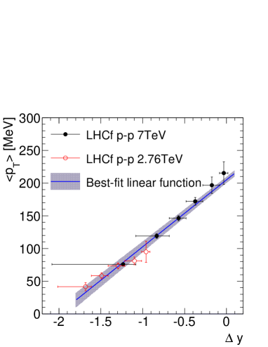
Figure 7: (color online). Average $p_{\text{T}}$ as a function of rapidity loss $\Delta y$. Filled circles indicate the LHCf results in $p$–$p$ collisions at $\sqrt{s}=$$7\text{\,}\mathrm{TeV}$ taken from Ref. LHCfpi0 . Open circles indicate the LHCf results in $p$–$p$ collisions at $\sqrt{s}=$$2.76\text{\,}\mathrm{TeV}$. The best-fit linear function to the LHCf data is shown by the solid line.

References

- (1) I. Abt, et al. (H1 Collaboration), Nucl. Phys. B 407, 515 (1993).
- (2) M. Derrick, et al. (ZEUS Collaboration), Phys. Lett. B 316, 412 (1993).
- (3) I. Arsene, et al. (BRAHMS Collaboration), Phys. Rev. Lett 93, 242303 (2004).
- (4) J. Adams, et al. (STAR Collaboration), Phys. Rev. Lett 97, 152302 (2006).
- (5) B. Abelev, et al. (ALICE Collaboration), Phys. Rev. Lett. 110, 082302 (2013).
- (6) R. Aaij, et al. (LHCb Collaboration), arXiv:1308.6729 [nucl-ex].
- (7) A. Dumitru, L. Gerland, and M. Strikman, Phys. Rev. Lett. 90, 092301 (2003).
- (8) J. Jalilian-Marian and A. H.Rezaeian, Phys. RevD. 85, 014017 (2012.)
- (9) J. L. Albacete, A. Dumitrub, H. Fujii, and Y. Nara, Nucl. Phys. A 897, 1-27 (2013).
- (10) A. Letessier-Selvon and T. Stanev, Rev. Mod. Phys. 83, 907-942 (2011).
- (11) LHCf Technical Design Report, CERN-LHCC-2006-004
- (12) O. Adriani, et al. (LHCf Collaboration), JINST, 3, S08006 (2008).
- (13) O. Adriani, et al. (LHCf Collaboration), JINST, 5, P01012.
- (14) W. C. Turner, E. H. Hoyer and N. V. Mokhov, Proc. of EPAC98, Stockholm, 368 (1998) http://accelconf.web.cern.ch/AccelConf/e98/contents.html. LBNL Rept. LBNL-41964 (1998).
- (15) T. Mase, et al. (LHCf Collaboration), NIM, A671, 129 (2012).
- (16) O. Adriani, et al. (LHCf Collaboration), Int. J. Mod. Phys. A, 28, 1330036 (2013).
- (17) LHC Performance and Statistics, https://lhc-statistics.web.cern.ch/LHC-Statistics/.
- (18) O. Adriani, et al. (LHCf Collaboration), Phys. Lett. B 703, 128-134 (2011).
- (19) J. M. Jowett, et al., In Proceedings of IPAC2013, Shanghai, China.
- (20) F. W. Bopp, J. Ranft, R. Engel and S. Roesler, Phys. Rev. C77, 014904 (2008).
- (21) S. Ostapchenko, Nucl. Phys. Proc. Suppl. 151, 143 (2006).
- (22) K. Werner, F.-M. Liu and T. Pierog, Phys. Rev. C74, 044902 (2006).
- (23) J. W. Cronin, H. J. Frisch, M. J. Shochet, J. P. Boymond, P. A. Piroué, and R. L. Sumner, Phys. Rev. D 11, 3105 (1975).
- (24) C. A. Bertulani, S. R. Klein and J. Nystrand, Ann. Rev. of Nucl. and Part. Sci. 55, 271 (2005).
- (25) C. von Weizsäcker Z. Physik 88, 612 (1934); E. J. Williams, Phys. Rev. 45, 729 (1934).
- (26) A. Mücke, R. Engel, J.P. Rachen, R.J. Protheroe and T. Stanev. Comput. Phys. Comm., 124, 290 (2000).
- (27) K. Kasahara, Proc. of 24th Int. Cosmic Ray. Conf. Rome 1, 399 (1995). EPICS web page, http://cosmos.n.kanagawa-u.ac.jp/
- (28) K. Kawade, et al. (LHCf Collaboration), JINST, 9, P03016 (2014).
- (29) O. Adriani, et al. (LHCf Collaboration), Phys. Rev. D. 86, 092001 (2012).
- (30) G. D’Agostini, Nucl. Instrum. Meth. A 362, 487-498 (1995)
- (31) G. Vismara, CERN-SL-2000-056 BI (2000).
- (32) R. J. Glauber and G. Matthiae, Nucl. Phys. B 21 (1970).
- (33) D. d’Enterria, arXiv:0302016 [nucl-ex]. Updated information is available at http://dde.web.cern.ch/dde/glauber_lhc.htm.
- (34) O. Adriani, et al. (LHCf Collaboration), paper in preparation.
- (35) The CMS Collaboration, CMS Physics Analysis Summary, CMS-PAS-FSQ-13-006.
- (36) B. Abelev, et al. (ALICE Collaboration), arXiv:1405.1849 [nucl-ex], CERN-PH-EP-2014-031.
- (37) B. Abelev, et al. (ALICE Collaboration), Phys. Rev. Lett. 110, 032301 (2013).
- (38) D. Amati, A. Stanghellini. and S. Fubini, Nuovo Cimento 26, 896 (1962).
- (39) J. Benecke, T. T. Chou, C. N. Yang, and E. Yen, Phys. Rev. 188, 2159–2169 (1969).
- (40) R. P. Feynman, Phys. Rev. Lett. 23, 1415–1417 (1969).