Optimal Transport in Worldwide Metro Networks

Abstract

Metro networks serve as good examples of traffic systems for understanding the relations between geometric structures and transport properties. We study and compare 28 world major metro networks in terms of the Wasserstein distance, the key metric for optimal transport, and measures geometry related, e.g. fractal dimension, graph energy and graph spectral distance. The finding of power-law relationships between rescaled graph energy and fractal dimension for both unweighted and weighted metro networks indicates the energy costs per unit area are lower for higher dimensioned metros. In $L$ space, the mean Wasserstein distance between any pair of connected stations is proportional to the fractal dimension, which is in the vicinity of our theoretical calculations treated on special regular tree graphs. This finding reveals the geometry of metro networks and tree graphs are in close proximity to one another. In $P$ space, the mean Wasserstein distance between any pair of stations relates closely to the average number of transfers. By ranking several key quantities transport concerned, we obtain several ranking lists in which New York metro and Berlin metro consistently top the first two spots.

Public transportation networks are crucial for cities. In mega cities metro networks are major parts of transportation on which most city inhabitants rely for daily mobility. It is therefore vital to evaluate the overall transport performance of metro networks. Most related attempts focused on optimal routes design which turned this problem into an engineering one aiming at the optimization of multi-objective tasks. For instance, Mandl s1 considered three separate problems, assignment of passengers to routes, assignment of vehicles to routes and finding the vehicle routes in a given network. Yeung et al s2 derived a simple and generic routing algorithm capable of considering all individual path choices simultaneously, which has been tested on London underground network. So far little attention has been paid to a comprehensive, empirical study of performance of worldwide major metro networks (MNS) by comparing the geometry features at the system level. This is exactly the main target of our project.

In this report, we examined 28 major MNS worldwide (see supplementary materials (SM) for the complete list and the sources of data) to study the relations between geometric structures and transport properties. We present for MNS empirical measurements of (i) fractal dimension, (ii) graph energy and graph Laplacian energy, (iii) graph spectral distance, and (iv) the Wasserstein distance. Further analysis of the above measures yields for MNS (I) the power-law scaling between the energy (or Laplacian energy) per unit area and the fractal dimension, with lower energy (costs per unit area) for higher dimensioned networks, (II) the scaling between the Wasserstein distance and the fractal dimension, which is in the vicinity of the theoretical curve based on special regular tree graphs, and (III) the phylogenetic network which suggests the geometric kinship among different MNS. These findings lead to several rankings of key quantities transport related in which New York metro and Berlin metro consistently top the first two spots.

Our data samples were taken from official websites of MNS. We considered both unweighted metro networks (UMN) and weighted metro networks (WMN). Defined on edges, the weight $w_{\mathrm{AB}}$ of a given edge AB is the number of different metro lines which pass through stations A and B. Our key results were obtained in $L$ space, so was our main discussion. The sole quantity of interest in $P$ space is the Wasserstein distance s3 . We present the values of topological quantities such as the average degree $\langle k\rangle$, the clustering coefficient $C$, and the average number of transfers $A_{\mathrm{T}}$ etc. in Table S1 of the SM. From this table one can have an immediate impression of the general picture of the geometric patterns of the MNS. First, $\langle k\rangle$ is close to 2 for most MNS, which indicates the tree-like structures of MNS. Second, that the clustering coefficient being close to 0 clearly indicates that cycles are rare in most MNS. Third, for most MNS, the average strength $\langle s\rangle$ is nearly equal to $\langle k\rangle$, which implies weight does not play a significant role. Exceptions are Berlin, Hamburg, Melbourne, Milan, New York, Seoul, Valencia and Washington. Fourth, the density $\rho$ is very small, which marks the sparseness of the MNS.

It is straightforward that the MNS are fractal s4 ; s5 ; s6 ; s7 . Here we adopt the methods of fractal dimension on networks (see SM). Denote the fractal dimension by $D$. For UMN, $D$ ranges from 1.0895 (Montreal) to 1.8237 (New York). $D$ of Montreal is close to the dimension of a line, which is exactly indicated by the shape of its metro plan (see SM). $D$’s of UMN in Asia are all smaller than 1.5. Three European cities have $D$’s larger than 1.5, with Berlin 1.6548, Paris 1.6005 and Milan 1.5524. When it comes to WMN, New York still tops with $D$ =1.8120, followed by Milan with $D$ being 1.6801.

To have a better understanding of the geometry of the MNS, the spectral graph theory s8 ; s9 ; s10 ; s11 ; s12 ; s13 ; s14 and the graph energy theory s15 ; s16 ; s17 ; s18 were applied to our data. The former is an elegant application of differential geometry methods to discrete spaces and mainly deals with the spectra of eigenvalues of matrices topology concerned, such as adjacency matrix $A$ and Laplacian matrix $L$ (see SM). For a graph $G$ with $N$ vertices, the energy $E$ is defined as

$$E=\sum_{i}\mathinner{\!\left\lvert\lambda_{i}\right\rvert},$$ (1)

where $\lambda_{i}(i=1,2,\ldots,N)$ is the $i$-th eigenvalue of $A$ of $G$. The Laplacian energy $E_{L}$ of $G$ is defined in a similar way as

$$E_{L}=\sum_{i}\mathinner{\!\left\lvert\mu_{i}-\langle k\rangle\right\rvert},$$ (2)

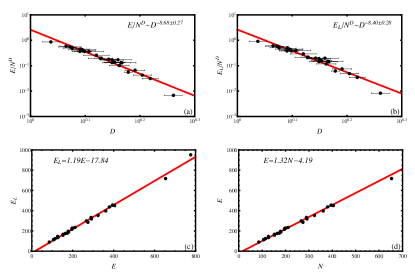
Fig. 1: For UMN there exists (a) the scaling between the rescaled energy$E/N^{D}$ and the fractal dimension $D$; (b) the scaling between the rescaled Laplacian energy $E_{L}/N^{D}$ and the fractal dimension $D$; (c) the linear relationship between the energy $E$ and the Laplacian energy $E_{L}$; (d) the linear dependence of the energy $E$ on the size $N$.

where $\mu_{i}(i=1,2,\ldots,N)$ is $i$-th eigenvalue of $L$ of $G$, and $\langle k\rangle$ is the average vertex degree of $G$. We studied $E$ and $E_{L}$ for both UMN (Fig. 1) and WMN (see SM). We only discussed the energy of UMN as similar analysis can be applied to WMN.

The first and also the major finding is the striking scaling between the rescaled energy $E/N^{D}$ and $D$

$$E/N^{D}\sim D^{-8.68\pm 0.27},$$ (3)

(see Fig. 1a), as well as the scaling between the rescaled Laplacian energy $E_{L}/N^{D}$ and $D$

$$E_{L}/N^{D}\sim D^{-8.40\pm 0.28},$$ (4)

(see Fig. 1b). The second finding is that $E$ and $E_{L}$ are almost identical (the two only differ slightly in scales) in describing the energy of a graph (Fig. 1c). Therefore we only focus on one of them, say $E$. The third finding is that both $E$ and $E_{L}$ scale as $N$ (Fig. 1d).

The second and third findings are not hard to interpret by checking the definitions of $E$ and $E_{L}$. But what kind of information can be extracted from the first finding? According to the graph energy theory, for a given $N$, the star graph with the fewest connections $N-1$ uniquely has the smallest energy $2\sqrt{N-1}$, and the complete graph owns the largest energy $2(N-1)$ (only exceeded by the very rare hyper-energetic graphs). MNS are neither star graphs, nor complete graphs and must be in the middle between these two extremes. For the MNS, more connections inevitably increase the construction costs. Therefore, one can treat $E$ as energy cost. $N^{D}$ is analogous to the area of a given metro with $N$ stations and fractal dimension $D$. Hence $E/N^{D}$ can be viewed as the energy cost per unit area for a given graph with parameters $E$, $N$, and $D$. For UMN, the highest value of $E/N^{D}$ is close to 0.8635, for Montreal, and the lowest value of $E/N^{D}$ is 0.0068, for New York. So by this criterion, the top 3 metros with the lowest energy costs per unit area are New York, Berlin and Paris. And in Asian metros, Seoul and Tokyo are the top 2. Delhi, Shenzhen, Taipei and Busan are on the bottom list with higher energy costs per unit area. For WMN, the ranking list of $E/N^{D}$ is nearly the same as the one for UMN.

To investigate the transport properties of the MNS, we employed the Wasserstein distance s19 ; s20 , the key metric in optimal transport theory. Consider two probability measures $\mu$ and $\nu$, with supports $\left\{x_{1},x_{2},\ldots,x_{n}\right\}$ and $\left\{y_{1},y_{2},\ldots,y_{m}\right\}$ respectively. Then the Wasserstein distance between $\mu$ and $\nu$ is defined as

$$W_{1}(\mu,\nu)=\inf\limits_{\begin{subarray}{c}\xi\\ \sum_{j}\xi(x_{i},y_{j})=\mu(x_{i})\\ \sum_{i}\xi(x_{i},y_{j})=\nu(y_{j})\end{subarray}}\sum_{i,j}c(x_{i},y_{j})\xi(x_{i},y_{j}),$$ (5)

where $c(x,y)$ is the cost of transporting one unit of mass from point $x$ to point $y$, and $\xi$ is a transfer plan between its margins $\mu$ and $\nu$.

We calculated the Wasserstein distances for the MNS in both $L$ space and $P$ space. In $L$ space, we calculated the mean values of $W_{1}(x,y)$, denoted by $\vbox{\hrule height=0.4pt\kern 1.50696pt\hbox{\kern-1.00006pt$W$\kern-1.00006pt}}_{1}^{L}$, between any pair of stations which are directly connected. In principle, one can also calculate the mean values of $W_{1}(x,y)$ between any two stations within the system. But as $W_{1}(x,y)$ is a quantity for measuring the local geometric structure, $W_{1}(x,y)$ for nodes further away does not significantly relate to the transport properties. We found a scaling of $\vbox{\hrule height=0.4pt\kern 1.50696pt\hbox{\kern-1.00006pt$W$\kern-1.00006pt}}_{1}^{L}$ versus $D$, with larger distance for higher dimension (Fig. 2a). The largest $\vbox{\hrule height=0.4pt\kern 1.50696pt\hbox{\kern-1.00006pt$W$\kern-1.00006pt}}_{1}^{L}$ comes from New York, being 1.2880, and the smallest one comes from Melbourne, being 1.0653.

As for most MNS the mean degree $\langle k\rangle$ approximates 2, it is then natural to relate MNS to tree graphs. For the sake of calculation, we consider a special class of homogeneous tree graphs, in which $\vbox{\hrule height=0.4pt\kern 1.50696pt\hbox{\kern-1.00006pt$W$\kern-1.00006pt}}_{1}^{L}$, $D$ and their relationship

$$\vbox{\hrule height=0.4pt\kern 1.50696pt\hbox{\kern-1.00006pt$W$\kern-1.00006pt}}_{1}^{L}=1+\frac{2(2^{D}-2)}{2^{D}(2^{D}-1)},$$ (6)

can be exactly obtained (see SM). In Fig. 2a, it can be seen that the theoretical curve for regular trees of interest is close to the empirical results by using our data. This observation confirms again the similarity in geometry between tree graphs and the MNS. We also notice that for most MNS, the empirical data points are below the theoretical values. This means that for any given $D$, the MNS have better transport properties than the homogeneous trees constructed by having smaller $\vbox{\hrule height=0.4pt\kern 1.50696pt\hbox{\kern-1.00006pt$W$\kern-1.00006pt}}_{1}^{L}$, the mean transport cost.

How do we understand the feature of the relationship between $\vbox{\hrule height=0.4pt\kern 1.50696pt\hbox{\kern-1.00006pt$W$\kern-1.00006pt}}_{1}^{L}$ and $D$? The Wasserstein distance $W_{1}(x,y)$ for an edge $xy$ increases when $D$ becomes larger. But for $\vbox{\hrule height=0.4pt\kern 1.50696pt\hbox{\kern-1.00006pt$W$\kern-1.00006pt}}_{1}^{L}$ on a homogeneous tree this behavior depends on how large $D$ is. Recall by the formula (see SM), $W_{1}(x,y)$ takes constant values 1 on the leaves and larger values $3-\frac{4}{k}$ on the other edges. Therefore, for $\vbox{\hrule height=0.4pt\kern 1.50696pt\hbox{\kern-1.00006pt$W$\kern-1.00006pt}}_{1}^{L}$, those non-leaf edges play the main role. However the fraction of non-leaf edges in the whole edge set of a homogeneous tree will decrease very quickly as $D$ or $k$ becomes very large. Hence when $D$ is large enough, this decreasing of the fraction of non-leaf edges will balance the increasing of the Wasserstein distance. Therefore, we observe a peak in the theoretic curve.

In $P$ space, $\vbox{\hrule height=0.4pt\kern 1.50696pt\hbox{\kern-1.00006pt$W$\kern-1.00006pt}}_{1}^{P}$ was calculated between any pair of stations. It is shown in Fig. 2b that $\vbox{\hrule height=0.4pt\kern 1.50696pt\hbox{\kern-1.00006pt$W$\kern-1.00006pt}}_{1}^{P}$ is linearly proportional to the average transfer $A_{\mathrm{T}}$, which is rather straightforward. As known in $P$ space, a single line is a complete subgraph. Therefore, $W_{1}(x,y)$ between any two stations pertaining to the same line is simply 1 according to its definition. For two stations which do not belong to the same line, the number of transfers shall concern in calculating $\vbox{\hrule height=0.4pt\kern 1.50696pt\hbox{\kern-1.00006pt$W$\kern-1.00006pt}}_{1}^{P}$. Hence in $P$ space, $\vbox{\hrule height=0.4pt\kern 1.50696pt\hbox{\kern-1.00006pt$W$\kern-1.00006pt}}_{1}^{P}$ measures the convenience of transfer a certain metro generally provides. Larger $\vbox{\hrule height=0.4pt\kern 1.50696pt\hbox{\kern-1.00006pt$W$\kern-1.00006pt}}_{1}^{P}$ states more transfers and smaller $\vbox{\hrule height=0.4pt\kern 1.50696pt\hbox{\kern-1.00006pt$W$\kern-1.00006pt}}_{1}^{P}$, less.

Intuitively we know that the MNS are all somewhat unique in geometric structures. But to quantitatively justify such differences we shall resort to specialized techniques in graph spectra theory. We have obtained graph spectra for all the MNS (see Fig. S10 of SM for examples). If one compares the spectra of Berlin metro and Paris metro, the gap is big. But when it comes to the spectra of Beijing metro and Berlin metro, these two are quite similar. To capture the distinctions, the spectral distances based on the normalized Laplacian were calculated and grouped, for the phylogenetic reconstruction s21 , aiming at identifying the relationships in geometric structure of the MNS. The quality of this reconstruction strongly depends on the distance matrix. The phylogenetic network of the MNS is shown in Fig. 3. As seen, most of the MNS in European cities are clustered, indicating the geometry kinship of these networks. The MNS in Guangzhou, Shanghai, Shenzhen and Beijing are close to each other, which manifests the proximity of designs of these metros. Fixing a certain metro, say New York, one can roughly estimate from the phylogenetic tree which of the rest metros is the closest, the next closest and the next to the next closest, so on and so forth. The list then goes like this: New York$\rightarrow$Milan$\rightarrow$Berlin…

We now compare the key quantities for all MNS to obtain a series of ranking lists. For any given metro network, if the ranking orders for different quantities are consistent, then the ranking lists can be used to evaluate the transport properties of the network of interest. For UMN, the ranking lists are $E/N^{D}$, $A_{\mathrm{T}}/N_{\mathrm{L}}$, $\vbox{\hrule height=0.4pt\kern 1.50696pt\hbox{\kern-1.00006pt$W$\kern-1.00006pt}}_{1}^{P}/N_{\mathrm{L}}$, $\vbox{\hrule height=0.4pt\kern 1.50696pt\hbox{\kern-1.00006pt$W$\kern-1.00006pt}}_{1}^{L}/D$ and $\rho$. Here $N_{\mathrm{L}}$ is the number of lines. For WMN, the ranking lists are $E/N^{D}$ and $A_{\mathrm{T}}/N_{\mathrm{L}}$. To ensure the consistency, all the lists are ranked from the highest to the lowest, regarding the performance. By this convention, better performance corresponds to smaller values of ranked quantities. $E/N^{D}$ is the energy cost, $A_{\mathrm{T}}/N_{\mathrm{L}}$ is the transfer time cost, $\vbox{\hrule height=0.4pt\kern 1.50696pt\hbox{\kern-1.00006pt$W$\kern-1.00006pt}}_{1}^{P}/N_{\mathrm{L}}$ and $\vbox{\hrule height=0.4pt\kern 1.50696pt\hbox{\kern-1.00006pt$W$\kern-1.00006pt}}_{1}^{L}/D$ are the transport cost, and $\rho$ is the construction cost. From Table 1, New York and Berlin top the first two spots consistently. Melbourne, Milan, Paris and Seoul are highly performed after New York and Berlin. Busan and Montreal are on the bottom spots. Here we are certainly not suggesting that New York is the best metro and Montreal is the worst. Rather, according to our criterion, New York and Berlin provide some efficient structures which might be more beneficial for transport. It is expected that this may shed some light on the planning of future metros.

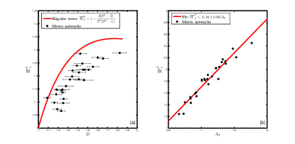
Fig. 2: The mean Wasserstein distance between connected stations $\vbox{\hrule height=0.4pt\kern 1.50696pt\hbox{\kern-1.00006pt$W$\kern-1.00006pt}}_{1}^{L}/D$ versus the fractal dimension $D$, in $L$ space. The solid curve indicates the same measurement treated on homogeneous trees. Data points being below the curve implies that any given metro network has better transport features than the regular tree with the same $D$. (b) The mean Wasserstein distance between any two stations $\vbox{\hrule height=0.4pt\kern 1.50696pt\hbox{\kern-1.00006pt$W$\kern-1.00006pt}}_{1}^{P}/N_{\mathrm{L}}$ versus the average number of transfers $A_{\mathrm{T}}$. The linear dependence of the two implies that in $P$ space, $\vbox{\hrule height=0.4pt\kern 1.50696pt\hbox{\kern-1.00006pt$W$\kern-1.00006pt}}_{1}^{P}/N_{\mathrm{L}}$ simply specifies the convenience of metro networks in regard of transfers needed.

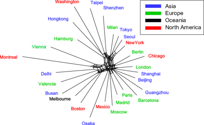
Fig. 3: The phylogenetic reconstruction of 28 metro networks, in which the graph distances among metro networks were visualized in a planar graph. The clustering of certain metros may reveal the geometry kinship among the communities.

Supplementary Materials:
Materials and Methods
Figures S1-S10
Tables S1-S3
References[1-8]

UMN					WMN
$E_{L}/N^{D}$	$A_{\mathrm{T}}/N_{\mathrm{L}}$	$\vbox{\hrule height=0.4pt\kern 1.05487pt\hbox{\kern-0.70004pt$W$\kern-0.70004pt}}_{1}^{P}/N_{\mathrm{L}}$	$\vbox{\hrule height=0.4pt\kern 1.05487pt\hbox{\kern-0.70004pt$W$\kern-0.70004pt}}_{1}^{L}/D$	$\rho$	$E_{L}/N^{D}$	$A_{\mathrm{T}}/N_{\mathrm{L}}$
0.0083 (New York)	0.0420 (New York)	0.0760 (New York)	0.7063 (New York)	0.0042 (New York)	0.0107 (New York)	0.0768 (New York)
0.0345 (Berlin)	0.0437 (Berlin)	0.0765 (Berlin)	0.7654 (Berlin)	0.0046 (Seoul)	0.0500 (Paris)	0.0857 (Berlin)
0.0492 (Paris)	0.0545 (Melbourne)	0.0907 (Melbourne)	0.7940 (Paris)	0.0076 (Berlin)	0.0510 (Milan)	0.0878 (Melbourne)
0.0613 (Seoul)	0.0576 (Seoul)	0.0945 (Seoul)	0.0796 (Milan)	0.0079 (Paris)	0.0546 (Berlin)	0.1246 (Hamburg)
0.0744 (Milan)	0.0606 (London)	0.0972 (London)	0.8095 (Moscow)	0.0082 (London)	0.0847 (Seoul)	0.1295 (Milan)
0.1171 (London)	0.0611 (Paris)	0.1059 (Paris)	0.8112 (Seoul)	0.0083 (Madrid)	0.1199 (Tokyo)	0.1415 (Seoul)
0.1434 (Barcelona)	0.0622 (Milan)	0.1067 (Milan)	0.8331 (Barcelona)	0.0088 (Shanghai)	0.128o (London)	0.1449 (Paris)
0.1455 (Madrid)	0.0702 (Hamburg)	0.1191 (Hamburg)	0.8427 (Madrid)	0.0095 (Melbourne)	0.1366 (Barcelona)	0.1521 (London)
0.1494 (Moscow)	0.0776 (Tokyo)	0.1328 (Madrid)	0.8431 (London)	0.0099 (Beijing)	0.1406 (Madrid)	0.1583 (Washington)
0.1582 (Tokyo)	0.0819 (Madrid)	0.1390 (Tokyo)	0.8603 (Hamburg)	0.0105 (Milan)	0.1538 (Moscow)	0.1735 (Tokyo)
0.1850 (Hamburg)	0.0840 (Moscow)	0.1411 (Moscow)	0.8636 (Osaka)	0.0112 (Tokyo)	0.1575 (Hamburg)	0.1824 (Chicago)
0.1968 (Osaka)	0.0873 (Shanghai)	0.1443 (Shanghai)	0.8653 (Melbourne)	0.0139 (Mexico)	0.1976 (Mexico)	0.2005 (Moscow)
0.1976 (Mexico)	0.0923 (Barcelona)	0.1457 (Barcelona)	0.8766 (Boston)	0.0145 (Chicago)	0.2185 (Beijing)	0.2071 (Shanghai)
0.2132 (Shanghai)	0.0930 (Chicago)	0.1569 (Beijing)	0.8857 (Valencia)	0.0148 (Valencia)	0.2222 (Osaka)	0.2120 (Osaka)
0.2167 (Beijing)	0.0986 (Beijing)	0.1671 (Chicago)	0.8918 (Mexico)	0.0148 (Delhi)	0.2318 (Shanghai)	0.2162 (Madrid)
0.2908 (Chicago)	0.1019 (Mexico)	0.1688 (Mexico)	0.8929 (Shanghai)	0.0151 (Hamburg)	0.3284 (Chicago)	0.2330 (Barcelona)
0.3797 (Valencia)	0.1041 (Osaka)	0.1879 (Valencia)	0.8993 (Chicago)	0.0156 (Moscow)	0.3955 (Vienna)	0.2591 (Mexico)
0.3820 (Melbourne)	0.1103 (Washington)	0.1885 (Taipei)	0.9001 (Delhi)	0.0164 (Guangzhou)	0.4110 (Guangzhou)	0.2596 (Valencia)
0.3954 (Vienna)	0.1162 (Valencia)	0.1907 (Boston)	0.9027 (Tokyo)	0.0164 (Barcelona)	0.4192 (Melbourne)	0.2971 (Beijing)
0.4110 (Guangzhou)	0.1246 (Boston)	0.1908 (Osaka)	0.9066 (Beijing)	0.0172 (Busan)	0.4709 (Boston)	0.2998 (Shenzhen)
0.4194 (Boston)	0.1358 (Taipei)	0.2066 (Washington)	0.9074 (Vienna)	0.0178 (Boston)	0.5087 (Delhi)	0.3588 (Boston)
0.4545 (Washington)	0.1499 (Shenzhen)	0.2206 (HongKong)	0.9120 (Guangzhou)	0.0183 (Shenzhen)	0.5391 (Hong Kong)	0.4215 (Vienna)
0.4883 (Hong Kong)	0.1516 (Guangzhou)	0.2295 (Delhi)	0.9230 (Washington)	0.0204 (Taipei)	0.5691 (Shenzhen)	0.4245 (Montreal)
0.5086 (Delhi)	0.1530 (HongKong)	0.2374 (Guangzhou)	0.9279 (Hong Kong)	0.0240 (Vienna)	0.5837 (Taipei)	0.4327 (Guangzhou)
0.5691 (Shenzhen)	0.1573 (Delhi)	0.2879 (Shenzhen)	0.9451 (Busan)	0.0241 (Osaka)	0.6086 (Busan)	0.4480 (Delhi)
0.5837 (Taipei)	0.1815 (Vienna)	0.3111 (Montreal)	0.9568 (Taipei)	0.0241 (Washington)	0.6741 (Valencia)	0.4750 (Taipei)
0.6086 (Busan)	0.1827 (Montreal)	0.3181 (Vienna)	0.9686 (Shenzhen)	0.0250 (HongKong)	0.8904 (Washington)	0.4923 (HongKong)
0.9114 (Montreal)	0.1845 (Busan)	0.3213 (Busan)	1.0242 (Montreal)	0.0303 (Montreal)	0.9114 (Montreal)	0.6610 (Busan)

Table 1: Ranking of key quantities for UMN (unweighted metro networks) and WMN (weighted metro networks). $E_{L}/N^{D}$: the average Laplacian energy per area; $A_{\mathrm{T}}/N_{\mathrm{L}}$: the average number of transfers per line; $\vbox{\hrule height=0.4pt\kern 1.50696pt\hbox{\kern-1.00006pt$W$\kern-1.00006pt}}_{1}^{L}/D$: the ratio of mean Wasserstein distance in $L$ space to fractal dimension $D$; $\vbox{\hrule height=0.4pt\kern 1.50696pt\hbox{\kern-1.00006pt$W$\kern-1.00006pt}}_{1}^{P}/N_{\mathrm{L}}$: the ratio of mean Wasserstein distance to the number of lines $N_{\mathrm{L}}$; $\rho$: the density of networks.

Acknowledgements: The source of data presented in this paper can be retrieved in the supplementary materials. W. L. would like to thank Prof. Jost for the hospitality during his stay in Leipzig where part of this work was done. This work was partially supported by the National Natural Science Foundation of China under grant No. 10975057, the Programme of Introducing Talents of Discipline to Universities under Grant No. B08033, and Engineering And Physical Sciences Research Council under grant No. EP/K016687/1. The authors declare no competing financial interests.

References

- (1) C.E. Mandl, Eur. J. Oper. Res. 5, 396-404 (1980).
- (2) C.H. Yeung, D. Saad, and K.Y.M. Wong, Proc. Natl. Acad. Sci. USA 7, 1301111110(2013).
- (3) C. Villani, Optimal Transport, Old and New, Springer-Verlag (Berlin, 2008).
- (4) B. Krön, J. Grap. Theo. 45, 224-239 (2004).
- (5) C. Ferber and Y. Holovatch, Eur. Phy. J. ST 216, 49-55 (2013).
- (6) C. Song, S. Havlin, and H. A. Makse, Nature (London) 433, 392 (2005).
- (7) C.M. Schneider, T.A. Kesselring, J.S. Andrade Jr., and H.J. Herrmann, Phys. Rev. E 86, 016707 (2012).
- (8) R. Grone, R. Merris, V.S. Sunder, SIAM J. Matrix Anal. Appl.11, 218–238 (1990).
- (9) F. Bauer, J. Jost and S. Liu, Math. Res. Lett. 19, 1185–1205(2012).
- (10) F. R. K. Chung, Spectral graph theory, CBMS Regional Conference Series in Mathematics, 92, 1997.
- (11) Y. Lin and S. T. Yau, Math. Res. Lett. 17, 343-356 (2010).
- (12) F. Bauer and J. Jost, Comm. Anal. Geom. 21, 787–845(2013).
- (13) A. Banerjee and J. Jost, Linear Algebra Appl. 428, 3015-3022 (2008).
- (14) F. R. K. Chung, L. Y. Lu and V. Vu, Proc. Natl. Acad. Sci. USA 100, 6313-6318 (2003).
- (15) I. Gutman, Berl. Math. Stat. Sekt. Fors. Graz 103, 1978.
- (16) I. Gutman, The energy of a graph: old and new results, in: A. Betten, A. Kohnert, R. Laue, A. Wassermann (Eds.), Algebraic Combinatorics and Applications, Springer-Verlag, Berlin, pp.196–211 (2001).
- (17) R. Balakrishnan, Linear Algebra Appl. 387, 287–295 (2004).
- (18) I. Gutman and B. Zheng, Linear Algebra Appl. 414, 29–37 (2006).
- (19) L. Wasserstein, Problems of Information Transmission 5, 47-82 (1969).
- (20) J. Jost and S. Liu, Discrete Comp. Geom. 51, 300-322 (2014).
- (21) D. H. Huson and D. Bryant, Mol. Biol. Evol., 23, 254-267 (2006).