An acoustic space-time and the Lorentz transformation in aeroacoustics

Abstract

In this paper we introduce concepts from relativity and geometric algebra to aeroacoustics. We do this using an acoustic space-time transformation within the framework of sound propagation in uniform flows. By using Geometric Algebra we are able to provide a simple geometric interpretation to the space-time transformation, and are able to give neat and lucid derivations of the free-field Green’s function for the convected wave equation and the Doppler shift for a stationary observer and a source in uniform rectilinear motion in a uniform flow.

Keywords: convected wave equation, geometric algebra, acoustic space-time

   ntroduction

This is a curiosity driven study that aims to explore the applicability of concepts from relativity and geometric algebra in the field of aeroacoustics. The analogy of acoustics with relativity has been investigated in physics and cosmology, but less has been done to use this work in the field of aeroacoustics. Geometric algebra has been successfully applied to a variety of fields but aeroacoustics has not yet been one of these. In order to introduce these concepts we make use of the simple problem of sound propagation in a uniform flow. Even though this problem is well understood, we show that by using the new concepts presented in this paper, we obtain a new geometric interpretation of the transformation that relates sound propagation in a uniform flow to the no flow case.

1.1   Analogies with Relativity

There is a substantial body of work in physics and cosmology on the analogies between general relativity and noise propagation in fluid flows. Much of it is fundamental and originates from the seminal work of Unruh [1] who identified the analogy between black holes and noise propagation in supersonic flows. Several other analogies exist between the relativistic physics of black holes and cosmology and various engineering disciplines, including optics and electrical engineering [2]. These analogies have resulted in the creation of several analogue space-times. The use of these analogues has so far been largely restricted to physicists attempting to gain a better understanding of gravity and quantum mechanics [3, 4]. This has recently changed with the recognition that engineers can benefit from the insights and techniques developed by physicists to deepen their own understanding and develop new technologies. Applying general relativity to optics has given birth to the field of Transformation Optics [5, 6] which has led to the development of perfect lenses and electromagnetic cloaks [6] using metamaterials, and has since stimulated similar studies on acoustic cloaks [7, 8, 9]. Relativity has also been applied successfully in electrical engineering [10, 11].

In this paper we introduce an analogy between relativity and aeroacoustics within the context of sound propagation in a uniform flow. We make extensive use of an acoustic space-time that provides a geometric interpretation of the transformation approach to solving the convected wave equation. We demonstrate the geometry established by a uniform flow field and use this to explain the form of the Green’s function for the convected wave equation [12], as well as the appearance of Doppler shifts [13, 14] and convective amplification.

1.2   Geometric Algebra

Geometric Algebra (GA) makes it easier to draw an analogy between relativity and aeroacoustics. GA was pioneered by Hestenes [15, 16] in the 1960s; this work took the algebras of Clifford and Grassmann [17, 18] and developed them into a powerful geometric language for mathematics and physics. Since the 1960s GA has been used in many physics and engineering applications. The key feature of GA is its ability to express physical equations in a coordinate-free form; the algebra is also extendible to any dimension. In this way GA is able to subsume complex numbers, quaternions, tensors etc. and provide simple and intuitive geometric interpretations of objects and often operators. GA has been applied successfully in electromagnetism [19, 20, 21], where the electric and magnetic fields are written as one geometric quantity and the four Maxwell’s equations are then reduced to a single equation. It has also been used for analysis of conformal arrays in radar and sonar applications [22]. Given the analogies between acoustics and electromagnetism [23, 24], it might seem reasonable to suppose that aeroacoustics might also benefit from a GA approach. While GA has been used in information engineering [25] and mechanical engineering [26] there have been few attempts at applying it in fluid mechanics. This paper is the first attempt at applying the language of GA to aeroacoustics. While much of the analysis for this paper was derived in GA, the reader will only explicitly need GA in §4. Other GA functionality which is required is given in the Appendices.

1.3   Sound In a Uniform Flow

In order to make use of the concepts introduced above, we consider the classic problem of sound propagation in a uniform flow. The equivalent problem of analysing the sound from the moving source was studied in the context of electromagnetics in the early 20th century, for example see Stratton [27], who gave the resulting signal amplitude distributions relative to the source either at time of emission or reception. Lighthill later gave the sound distributions in the context of acoustics [28, §4.1]. Lighthill effectively solved for the sound field in the frame of the fluid, then used a Galilean transformation to find the solution in the frame of the observer in which flow is present [28, Eq. (16)]. Lighthill also gave some physical interpretation of the result in the fluid frame. A clear treatment of this approach is given by Dowling and Williams [29, §9].

More recently, the problem has been solved by considering the convected wave equation, and using a Lorentz-type transform [30, §9.1.1]. This is useful because the non-convected wave equation is easily solved using an appropriate Green’s function. This latter approach has been used to develop a wide range of aeroacoustic theories in active control [31], duct acoustics [32, 33], aerofoil broadband noise [12, 34, 35], and aerodynamic theories on thin aerofoils in compressible flows [36, 37]. The transforms used in these methods have been summarised by [38].

However, the physical interpretation of this transformation approach is not clear, with the transform itself generally simply stated in terms of similarity variables with little justification as to where the transformation originates from and how it can be generalised to other problems. For example, it is not clear how the theory of Blandeau et al [39] on trailing edge noise for rotating blades, which neglects the uniform mean flow effects, can be extended to take these effects into account; Sinayoko et al [40] therefore resorted to solving the same problem from first principles without the use of transformations.

Addressing this shortcoming, and providing an interpretation of the transformation method is the main goal of this paper. We shall see that this method differs from that of Lighthill and Dowling et al in that the solution is found not in the frame of the fluid, but in a third frame that moves with the observer and where the wave operator takes a simple form. The advantage over Lighthill’s method is that boundary conditions that are given in the observer frame can be more easily applied in the new third frame, which we shall refer to as the Lorentzian frame because this is the type of transform required to produce it.

1.4   Organisation of the Paper

The paper is organised as follows. §2 defines the acoustic space-time and introduces the observer, fluid and Lorentzian frames as well as the associated time-space coordinates and transformations. §2.2 provides the reciprocal frequency-wavenumber coordinates and transformations. These transformations are used to derive simple solutions for three classic aeroacoustic problems in §3: the free field Green’s function for the convected wave equation in a uniform flow; the Doppler shift for a stationary observer and a source in uniform rectilinear motion in a uniform flow; providing a comparison with previous work and examples of the advantages of our approach. §4 introduces the language of Geometric Algebra and shows how it provides new insights into the geometry underlying the transformations and the nature of the wave operator.

   ransforming the convected wave equation in space-time coordinates

Let $(x,y,z)$ be Cartesian coordinates in a Euclidean space, and $p(x,y,z,t)$ be a scalar function of position and time $t$ that represents the perturbation to the pressure in a fluid occupying the space. If the background pressure and density of the fluid are constant, and the fluid is stationary, the perturbation pressure must satisfy [41],

$$\left[\frac{\partial^{2}}{\partial x^{2}}+\frac{\partial^{2}}{\partial y^{2}}+\frac{\partial^{2}}{\partial z^{2}}-\frac{1}{c^{2}}\frac{\partial^{2}}{\partial t^{2}}\right]p=-f,$$ (1)

where $f(x,y,z,t)$ is a scalar function that represents the sound sources in the fluid, and $c$ is the (constant) speed of sound in the fluid. If instead there is a uniform background flow with velocity $U$ in the $z$ direction, then $p$ must satisfy,

$$\left[\frac{\partial^{2}}{\partial x^{2}}+\frac{\partial^{2}}{\partial y^{2}}+\frac{\partial^{2}}{\partial z^{2}}-\frac{1}{c^{2}}\left(\frac{\partial}{\partial t}+U\frac{\partial}{\partial z}\right)^{2}\right]p=-f.$$ (2)

We will present and interpret a transformation that allows us to solve Eqn (2) by transforming it into Eqn (1), solving that, and then transforming back. This transformation has been presented most recently in an alternative form by [38] and has been used prior to this, for example in [42, 43], however, in previous presentations, no interpretation of the transformation was given. We rectify this using the concept of a newly defined “acoustic space-time” that is analogous to the special relativistic space-time of physics, but with the speed of light replaced by the speed of sound.

It will be immediately obvious to readers familiar with relativity that the wave equation is Lorentz invariant, but that the physical transformation between Eqn (1) and Eqn (2) is a Galilean transform, since the underlying physics is Newtonian. Usually this is regarded as a curiosity, however by making use of the Lorentz symmetry in a hyperbolic space we end up with a problem that is easier to solve. On top of this we can then construct non-orthogonal frames using the Galilean transformation to obtain solutions in terms of physical variables. Having introduced a hyperbolic background space it is natural to use Geometric Algebra, in which rotors provide a lucid way of handling Lorentz transformations, and the whole problem can be written in a coordinate free form.

In the upcoming section the Galilean and Lorentz transformations are introduced in detail within an acoustic space-time. Readers already familiar with this can move on to the description of how the space-time can be used to interpret transformations in the frequency-wavenumber domain §2.2, applications §3, and the advantages provided by geometric algebra §4.

2.1   The Acoustic Space-Time

We will be concerned throughout the paper with vector spaces with dimension higher than 3, and more significantly, with mixed signature. The 3-dimensional Euclidean space usually used to model Newtonian mechanics can have an arbitrary set of basis vectors (a frame), denoted $\{\bm{e}_{i}\}$, which are defined relative to each other by the set of inner products,

$$\bm{e}_{i}\cdot\bm{e}_{j}.$$ (3)

To deal with spaces of higher dimension we simply need more basis vectors, but to deal with spaces of mixed signature we need to make one further generalisation. In Euclidean space the inner products $\bm{e}_{i}\cdot\bm{e}_{j}$ are all positive numbers. In a space of mixed signature this restriction is relaxed. In this article we deal with a 4-dimensional space in which we define a frame $\{\gamma_{\mu}^{\prime}\}$ that satisfies the simple space-time metric,

$$\gamma_{\mu}^{\prime}\cdot\gamma_{\nu}^{\prime}=\begin{bmatrix}1&0&0&0\\ 0&-1&0&0\\ 0&0&-1&0\\ 0&0&0&-1\end{bmatrix}\text{ where }\mu,\nu=t,x,y,z.$$ (4)

Note that we have not used bold font to denote these basis vectors. In general we reserve bold font for vectors in 3-dimensional Euclidean space. We have also switched from using Latin indices to using Greek indices. We reserve Latin indices for frames spanning 3-dimensional Euclidean space. This matrix of all the inner products of a frame is called the metric of the frame. Signature refers to the signs of the eigenvalues of the metric, which is a fundamental property of the space. We can see from this metric that there are a mixture of signs in the metric of space-time, hence the term mixed signature.

For any arbitrary frame $\{e_{\mu}\}$ it is possible to construct a reciprocal frame $\{e^{\mu}\}$ (see Appendix A) such that,

$$e_{\mu}\cdot e^{\nu}=\delta^{\nu}_{\mu},\quad\delta^{\nu}_{\mu}=\left\{\begin{array}[]{ll}1&\mu=\nu\\ 0&\mu\neq\nu\end{array}\right.,$$ (5)

We use this reciprocal frame to find the coordinates of an arbitrary vector when the original frame is not orthonormal, as in this case. For our $\{\gamma_{\mu}^{\prime}\}$ frame, the reciprocal frame $\{{\gamma^{\mu}}^{\prime}\}$ is given by,

$${\gamma^{t}}^{\prime}=\gamma_{t}^{\prime},\quad{\gamma^{x}}^{\prime}=-\gamma_{x}^{\prime},\quad{\gamma^{y}}^{\prime}=-\gamma_{y}^{\prime},\quad{\gamma^{z}}^{\prime}=-\gamma_{z}^{\prime}.$$ (6)

An arbitrary four vector $\xi$ can be written in the $\{\gamma_{\mu}^{\prime}\}$ frame as,

$$\xi=ct^{\prime}\gamma_{t}^{\prime}+x^{\prime}\gamma_{x}^{\prime}+y^{\prime}\gamma_{y}^{\prime}+z^{\prime}\gamma_{z}^{\prime},$$ (7)

and the coordinates can be found using the reciprocal frame,

$$ct^{\prime}=\xi\cdot{\gamma^{t}}^{\prime},\quad x^{\prime}=\xi\cdot{\gamma^{x}}^{\prime},\quad y^{\prime}=\xi\cdot{\gamma^{y}}^{\prime},\quad z^{\prime}=\xi\cdot{\gamma^{z}}^{\prime}.$$ (8)

In this article we only deal with frames that are the same at every position in the vector space, and with spaces that are not curved. For these kinds of space the method used above for finding coordinates using the reciprocal frame works for any frame (see [19] and Appendix A). Note that the time coordinate has been factored into $c$ and $t^{\prime}$, where $c$ is the speed of sound in the fluid being considered, and $t^{\prime}$ has units of time.

2.1.1   Galilean Transform

Let us now define a second frame $\{\gamma_{\mu}\}$, using the scalar constant $M=U/c$, as,

$$\gamma_{t}=\gamma_{t}^{\prime}-M\gamma_{z}^{\prime},\quad\gamma_{x}=\gamma_{x}^{\prime},\quad\gamma_{y}=\gamma_{y}^{\prime},\quad\gamma_{z}=\gamma_{z}^{\prime}.$$ (9)

The reciprocal frame $\{\gamma^{\mu}\}$ is given by (see Eqn (88)),

$$\gamma^{t}=\gamma_{t}^{\prime},\quad\gamma^{x}=-\gamma_{x}^{\prime},\quad\gamma^{y}=-\gamma_{y}^{\prime},\quad\gamma^{z}=M\gamma_{t}^{\prime}-\gamma_{z}^{\prime}.$$ (10)

An arbitrary four vector $\xi$ can be written in the $\{\gamma_{\mu}\}$ frame as,

$$\xi=ct\gamma_{t}+x\gamma_{x}+y\gamma_{y}+z\gamma_{z},$$ (11)

and the coordinates can be found using the reciprocal frame,

$$ct=\xi\cdot{\gamma^{t}},\quad x=\xi\cdot{\gamma^{x}},\quad y=\xi\cdot{\gamma^{y}},\quad z=\xi\cdot{\gamma^{z}}.$$ (12)

From this point on we redefine $(x,y,z,t)$ as the coordinates of this frame in a four dimensional space-time defined below. We will see however that $(x,y,z,t)$ will still represent the space and time that are measurable by us, which is why we choose to retain these symbols. Using these expressions for the coordinates along with Eqn (8), we can show that the following coordinate transformations hold,

$$ct=ct^{\prime},\quad x=x^{\prime},\quad y=y^{\prime},\quad z=z^{\prime}+Mct^{\prime}.$$ (13)

From Eqn (13), if an observer is at constant $(x,y,z)$, then they are moving in the $-z$ direction with Mach number $M$ with respect to the $(x^{\prime},y^{\prime},z^{\prime})$ coordinates. We can say that $\{\gamma_{\mu}^{\prime}\}$ is the frame of the fluid, while $\{\gamma_{\mu}\}$ is the frame of the observer. It is clear that this is simply a Galilean transformation.

Let us now define the linear operator $\mathcal{L}$ that operates on fields in the acoustic space-time we have constructed, and write it in terms of the coordinates in the $\{\gamma_{\mu}^{\prime}\}$ frame,

$$\mathcal{L}=\frac{\partial^{2}}{\partial{x^{\prime}}^{2}}+\frac{\partial^{2}}{\partial{y^{\prime 2}}}+\frac{\partial^{2}}{\partial{z^{\prime 2}}}-\frac{1}{c^{2}}\frac{\partial^{2}}{\partial{t^{\prime 2}}}.$$ (14)

Using the chain rule and the coordinate transformations given in Eqn (13) we can show that $\mathcal{L}$ may be written as,

$$\mathcal{L}=\frac{\partial^{2}}{\partial x^{2}}+\frac{\partial^{2}}{\partial y^{2}}+\frac{\partial^{2}}{\partial z^{2}}-\frac{1}{c^{2}}\left(\frac{\partial}{\partial t}+U\frac{\partial}{\partial z}\right)^{2}.$$ (15)

If we consider the scalar functions $p(\xi)$ and $f(\xi)$, then the equation,

$$\mathcal{L}p=-f,$$ (16)

is exactly equivalent to Eqn (1) if $\mathcal{L}$ is written in the $\{\gamma_{\mu}^{\prime}\}$ frame, and equivalent to Eqn (2) if $\mathcal{L}$ is written in the $\{\gamma_{\mu}\}$ frame. Note that $p$ and $f$ are scalar functions of position in space-time, $\xi$. This four-vector can be parameterised in terms of the coordinates of any frame we introduce, and hence $p$ (and $f$) can be thought of as $p(\xi(x,y,z,t))$, or $p(\xi(x^{\prime},y^{\prime},z^{\prime},t^{\prime}))$ (we have omitted the factor of $c$ since it is a constant). In fact, $\mathcal{L}$ can be defined in a simple coordinate free manner using the vector derivative of Geometric Algebra. In addition, the use of Geometric Algebra for this purpose allows an intuitive explanation to be given as to why $\mathcal{L}$ takes a simple form in one frame, and a complex one in the other, as is explained in §4.4.

We have found a transformation that allows us to rewrite Eqn (2) as Eqn (1), however, if a source or observer is at rest in the $\{\gamma_{\mu}\}$ frame (i.e. they are at a constant $x$, $y$ and $z$), they will be in motion in the $\{\gamma_{\mu}^{\prime}\}$ frame. We would like to transform to a frame where the wave operator takes the simple form in Eqn (1), but where an observer or source that is stationary in the $\{\gamma_{\mu}\}$ frame is still stationary.

2.1.2   Lorentz Transform

Let us define the frame $\{\gamma_{\mu}^{\prime\prime}\}$ as,

$$\gamma_{t}^{\prime\prime}=\frac{1}{\beta}(\gamma_{t}^{\prime}-M\gamma_{z}^{\prime}),\quad\gamma_{x}^{\prime\prime}=\gamma_{x}^{\prime},\quad\gamma_{y}^{\prime\prime}=\gamma_{y}^{\prime},\quad\gamma_{z}^{\prime\prime}=\frac{1}{\beta}(\gamma_{z}^{\prime}-M\gamma_{t}^{\prime}),$$ (17)

where $\beta$ is defined by,

$$\beta=\sqrt{1-M^{2}}.$$ (18)

Note that it is simple to show that the $\{\gamma_{\mu}^{\prime\prime}\}$ frame satisfies the space-time metric in Eqn (4). The reciprocal frame $\{{\gamma^{\mu}}^{\prime\prime}\}$ is given by (see Eqn (88)),

$${\gamma^{t}}^{\prime\prime}=\gamma_{t}^{\prime\prime},\quad{\gamma^{x}}^{\prime\prime}=-\gamma_{x}^{\prime\prime},\quad{\gamma^{y}}^{\prime\prime}=-\gamma_{y}^{\prime\prime},\quad{\gamma^{z}}^{\prime\prime}=-\gamma_{z}^{\prime\prime}.$$ (19)

An arbitrary four vector $\xi$ can be written in the $\{\gamma_{\mu}^{\prime\prime}\}$ frame as,

$$\xi=ct^{\prime\prime}\gamma_{t}^{\prime\prime}+x^{\prime\prime}\gamma_{x}^{\prime\prime}+y^{\prime\prime}\gamma_{y}^{\prime\prime}+z^{\prime\prime}\gamma_{z}^{\prime\prime},$$ (20)

and the coordinates can be found using the reciprocal frame,

$$ct^{\prime\prime}=\xi\cdot{\gamma^{t}}^{\prime\prime},\quad x^{\prime\prime}=\xi\cdot{\gamma^{x}}^{\prime\prime},\quad y^{\prime\prime}=\xi\cdot{\gamma^{y}}^{\prime\prime},\quad z^{\prime\prime}=\xi\cdot{\gamma^{z}}^{\prime\prime}.$$ (21)

Using these expressions for the coordinates along with Eqn (8) and Eqn (12) we can derive the coordinate relations,

$$ct^{\prime\prime}=\frac{1}{\beta}(ct^{\prime}+Mz^{\prime}),\quad x^{\prime\prime}=x^{\prime},\quad y^{\prime\prime}=y^{\prime},\quad z^{\prime\prime}=\frac{1}{\beta}(z^{\prime}+Mct^{\prime}),$$ (22)

$$ct^{\prime\prime}=\beta ct+\frac{M}{\beta}z,\quad x^{\prime\prime}=x,\quad y^{\prime\prime}=y,\quad z^{\prime\prime}=\frac{z}{\beta}.$$ (23)

We note from the relations in Eqn (23) that if a source or observer is at constant $x,y,z$ they will also be at constant $x^{\prime\prime},y^{\prime\prime},z^{\prime\prime}$. Using the chain rule along with these relations, we can show that,

$$\mathcal{L}=\frac{\partial^{2}}{\partial{x^{\prime\prime}}^{2}}+\frac{\partial^{2}}{\partial{y^{\prime\prime 2}}}+\frac{\partial^{2}}{\partial{z^{\prime\prime 2}}}-\frac{1}{c^{2}}\frac{\partial^{2}}{\partial{t^{\prime\prime 2}}}.$$ (24)

We see that under the Lorentz transformation the wave equation is left unchanged. This will be obvious to readers familiar with relativity, and is particularly well explained in a coordinate free way using Geometric Algebra. The Lorentz transform can be shown very simply to be a generalised form of rotation §4.2, and hence leaves the metric unchanged. Keeping the metric unchanged automatically means that the operator $\mathcal{L}$, which can be written in a frame independent way using Geometric Algebra, remains simple, as is explained in §4.4.

For now though let us consider these transformations more carefully. Since $x$ and $y$ are unaffected, we can illustrate the transformation by considering only the $z$ and time directions (Figure 1).

Figure 1: The effect of the Galilean and Lorentz transforms on the basis vectors.

Conceptually we can think of our method as beginning by creating a frame that moves with the fluid. This frame is the $\{\gamma_{\mu}^{\prime}\}$ frame, and satisfies the space-time signature (Eqn (4)). This is why in Figure 1 this is the frame shown with its basis vectors orthogonal. The speed of sound is fundamental to this frame.

From this frame we then create two new frames, using either a Galilean or a Lorentz transform. To create the space with the Galilean transform we skew the time vector in the direction of the flow (this is the red frame in Figure 1), and leave the spatial vectors unchanged. The coordinates of this frame represent the coordinates that we observe if we sit still and see fluid flowing past us. In this frame the complex wave operator given in Eqn (15) applies.

The frame created using the Lorentz transform ($\{\gamma_{\mu}^{\prime\prime}\}$) has its time vector pointing in the same direction as that of the observer frame, but this frame must satisfy the space-time signature. Hence the time vector is stretched and the spatial vector must change (this is the green frame in Figure 1). It must be remembered when looking at Figure 1 that we are considering a hyperbolic space, so $\gamma_{t}^{\prime\prime}$ and $\gamma_{z}^{\prime\prime}$ are orthogonal. In this frame the simple wave operator applies, and we also have the important property that if an observer is at constant $x,y,z$ they are also at constant $x^{\prime\prime},y^{\prime\prime},z^{\prime\prime}$. This allows the conversion of boundary conditions from the $\{\gamma_{\mu}\}$ frame to the $\{\gamma_{\mu}^{\prime\prime}\}$ frame.

2.2   Transforming in the frequency-wavenumber domain

The ordinary wave equation takes a simpler algebraic form in the frequency-wavenumber domain,

$$\left[\frac{\omega^{2}}{c^{2}}-k^{2}\right]P(\bm{k},\omega)=F(\bm{k},\omega),$$ (25)

where $P$ is the Fourier transform of $p$, defined as,

$$P(\bm{k},\omega)=\int_{-\infty}^{\infty}\int_{\mathbb{R}^{3}}{p(\bm{x},t)e^{i(\omega t-\bm{k}\cdot\bm{x})}}d^{3}\bm{x}dt$$ (26)

and $F$ is the Fourier transform of $f$. Eqn (25) can be obtained by taking the Fourier transform of Eqn (1).

Similarly, the convected wave equation (Eqn (2)) takes a simpler algebraic form in the frequency-wavenumber domain,

$$\left[\left(\frac{\omega}{c}-Mk_{z}\right)^{2}-k^{2}\right]P(\bm{k},\omega)=F(\bm{k},\omega).$$ (27)

Eqn (27) can be converted into Eqn (25) by using an appropriate transformation. The main difference with the physical domain transformations is that, given a reference frame $\{\gamma_{\mu}\}$, the wavenumbers $k_{x}$, $k_{y}$ and $k_{z}$ and the frequency $\omega$ are the components of a 4-wavevector $\kappa$ defined in the reciprocal frame $\{\gamma^{\mu}\}$ as,

$$\kappa\equiv\frac{\omega}{c}{\gamma^{t}}-k_{x}{\gamma^{x}}-k_{y}{\gamma^{y}}-k_{z}{\gamma^{z}},$$ (28)

or, equivalently,

$$\omega/c \equiv\kappa\cdot\gamma_{t}, k_{x} \equiv-\kappa\cdot\gamma_{x}, k_{y} \equiv-\kappa\cdot\gamma_{y}, k_{z} \equiv-\kappa\cdot\gamma_{z}.$$ (29)

This definition of $\kappa$ is such that the phase $\phi\equiv\kappa\cdot\xi$ takes the usual form,

$$\phi=\omega t-k_{x}x-k_{y}y-k_{z}z,$$ (30)

irrespective of the reference frame.

Since we have already defined the fluid frame $\{\gamma_{\mu}^{\prime}\}$ and the Lorentzian frame $\{\gamma_{\mu}^{\prime\prime}\}$, we can readily obtain the wavevector coordinate transformations by applying Eqn (29) to the appropriate frame, which yields,

$$\omega^{\prime} =\omega-Mck_{z}, k_{z}^{\prime} =k_{z}, k_{x}^{\prime} =k_{x}, k_{y}^{\prime} =k_{y}.$$ (31)

for the fluid frame, and,

$$\omega^{\prime\prime} =\frac{1}{\beta}(\omega^{\prime}+Mck_{z}^{\prime})=\frac{\omega}{\beta},$$ (32)

$$k_{z}^{\prime\prime} =\frac{1}{\beta}\left(k_{z}^{\prime}+M\frac{\omega^{\prime}}{c}\right)=\beta k_{z}+\frac{M}{\beta}\frac{\omega}{c},$$ (33)

$$k_{x}^{\prime\prime} =k_{x}^{\prime}=k_{x},$$ (34)

$$k_{y}^{\prime\prime} =k_{y}^{\prime}=k_{y}.$$ (35)

for the Lorentzian frame.

Thus, from Eqn (31), the frequency depends on the axial wavenumber in the fluid frame ($\omega^{\prime}=\omega+Mck_{z}^{\prime}$), while the wavenumber components remain the same in the observer and the fluid frames ($k_{z}=k_{z}^{\prime}$, $k_{x}=k_{x}^{\prime}$ and $k_{y}=k_{y}^{\prime}$). This behaviour is the reverse of the way the physical coordinates transform between the observer and the fluid frames: time remains the same ($t=t^{\prime}$) while the axial coordinate changes ($z^{\prime}=z-Mct^{\prime}$).

Similarly, in the Lorentzian frame, the frequency $\omega^{\prime\prime}$ is fixed relative to the observer frequency $\omega$ while the axial wavenumber $k_{z}^{\prime\prime}$ is a linear combination of $k_{z}$ and $\omega$. In contrast, in the space-time domain, it is the axial Lorentzian position $z^{\prime\prime}$ that is fixed relative to the axial observer position $z$ ($z^{\prime\prime}=z/\beta$) while the Lorentzian time $t^{\prime\prime}$ is a linear combination of $z$ and $t$.

   pplications

3.1   Sound Propogation in Acoustic Space-Time Along Null Directions

Let us imagine a point marker on a wave front moving at the speed of sound $c$ relative to the fluid, and in any spatial direction. Written using the coordinates of the frame that moves with the fluid $\{\gamma_{\mu}^{\prime}\}$, the marker’s motion will be described by,

$$\sqrt{(x^{\prime}-x_{s}^{\prime})^{2}+(y^{\prime}-y_{s}^{\prime})^{2}+(z^{\prime}-z_{s}^{\prime})^{2}}=c(t^{\prime}-\tau^{\prime}),$$ (36)

if at time $\tau^{\prime}$ the point is at the position defined by $x_{s}^{\prime},y_{s}^{\prime},z_{s}^{\prime}$. It is important to note that the time of the frame that moves with the fluid is the same as the time of the frame of the observer (see Eqn (13)). The coordinates $x^{\prime},y^{\prime},z^{\prime},t^{\prime}$ define the marker’s progressive position in acoustic space-time, and $x_{s}^{\prime},y_{s}^{\prime},z_{s}^{\prime},\tau^{\prime}$ define the starting position of the marker. Therefore we can define the 4-vectors $\xi$ and $\eta$ such that,

$$\xi =ct^{\prime}\gamma_{t}^{\prime}+x^{\prime}\gamma_{x}^{\prime}+y^{\prime}\gamma_{y}^{\prime}+z^{\prime}\gamma_{z}^{\prime},$$ (37)

$$\eta =c\tau^{\prime}\gamma_{t}^{\prime}+x_{s}^{\prime}\gamma_{x}^{\prime}+y_{s}^{\prime}\gamma_{y}^{\prime}+z_{s}^{\prime}\gamma_{z}^{\prime}.$$

Once again, $\eta$ is the single position in space-time at which the marker on the wavefront starts, and $\xi$ is the collection of points at which the marker can end up if it moves at the speed of sound in any of the spatial directions.

We now consider the vector $\xi-\eta$, which points from the marker on the wavefront’s starting position to its current position, or in other words the vector tangent to the marker’s motion (this is analogous to a ray [45]). If we take the dot product of this vector with itself we obtain (using Eqn (4)),

$$(\xi-\eta)^{2}=c^{2}(t^{\prime}-\tau^{\prime})^{2}-(x^{\prime}-x_{s}^{\prime})^{2}-(y^{\prime}-y_{s}^{\prime})^{2}-(z^{\prime}-z_{s}^{\prime})^{2}.$$ (38)

Invoking Eqn (36) we see that,

$$(\xi-\eta)^{2}=0.$$ (39)

It is important to note at this point that we are not dealing with a Euclidean space, and so this does not imply that $\xi-\eta$ is a point. Instead it implies that $\xi-\eta$ is one of a set of vectors referred to as null vectors.

To conclude, if a point on a wavefront is moving relative to the fluid at the speed of sound, then the vector tangent to its motion in our space time is a null vector, this is in fact independent of frame. This is an important property of the acoustic space-time interpretation, and we shall see it again in the following sections.

3.2   Green’s function for the convected wave equation

The Green’s function for the convected wave equation satisfies,

$$\mathcal{L}G(\xi,\eta)=-\delta(\xi-\eta),$$ (40)

where $\mathcal{L}$ is given by Eqn (15), $\delta$ is a Dirac delta distribution, $\xi$ is a 4-vector giving the position of the observer in acoustic space-time, and $\eta$ a 4-vector giving the position of the source. We express these two 4-vectors in the observer frame $\{\gamma_{\mu}\}$ and the Lorentzian frame $\{\gamma_{\mu}\}^{\prime\prime}$ as,

$$\xi =ct\gamma_{t}+x\gamma_{x}+y\gamma_{y}+z\gamma_{z}=ct^{\prime\prime}\gamma_{t}^{\prime\prime}+x^{\prime\prime}\gamma_{x}^{\prime\prime}+y^{\prime\prime}\gamma_{y}^{\prime\prime}+z^{\prime\prime}\gamma_{z}^{\prime\prime},$$ (41)

$$\eta =c\tau\gamma_{t}+x_{s}\gamma_{x}+y_{s}\gamma_{y}+z_{s}\gamma_{z}=c\tau^{\prime\prime}\gamma_{t}^{\prime\prime}+x_{s}^{\prime\prime}\gamma_{x}^{\prime\prime}+y_{s}^{\prime\prime}\gamma_{y}^{\prime\prime}+z_{s}^{\prime\prime}\gamma_{z}^{\prime\prime}.$$

The relations between the double prime and no prime coordinates are given in §2.1.2. If we write $\mathcal{L}$ in the $\{\gamma_{\mu}^{\prime\prime}\}$ frame (Eqn (24)), Eqn (40) reduces to the ordinary wave equation for which the Green’s function is well known and is given by [46, §11.3],

$$G(\xi,\eta)=\frac{\delta\left(t^{\prime\prime}-\tau^{\prime\prime}-R^{\prime\prime}/c\right)}{4\pi R^{\prime\prime}},$$ (42)

where $R^{\prime\prime}\equiv\sqrt{(x^{\prime\prime}-x_{s}^{\prime\prime})^{2}+(y^{\prime\prime}-y_{s}^{\prime\prime})^{2}+(z^{\prime\prime}-z_{s}^{\prime\prime})^{2}}$. Looking carefully at the argument of the delta function, and recalling that the $\{\gamma_{\mu}^{\prime\prime}\}$ frame must satisfy the space-time signature (Eqn (4)), we see that in order for $G$ to be non-zero, we must have,

$$(\xi-\eta)^{2}=0.$$ (43)

Hence we see that the impulse is spreading out along the null directions of our acoustic space-time, as was discussed in §3.1. We can now express $G$ in the observer-frame from Eqn (23), which yields,

$$R^{\prime\prime} =\sqrt{(x-x_{s})^{2}+(y-y_{s})^{2}+(z-z_{s})^{2}/\beta^{2}},$$ (44)

$$t^{\prime\prime}-\tau^{\prime\prime} =\beta(t-\tau)+\frac{M}{\beta c}(z-z_{s}).$$

Substituting these results into Eqn (42) for $G$, we obtain an expression for $G$ in the observer coordinates. We can use this to obtain a solution to Eqn (2) for a general forcing $f(x,y,z,t)$,

$$p=\int_{x_{s}}\int_{y_{s}}\int_{z_{s}}\frac{f\left(x_{s},y_{s},z_{s},t+\frac{M}{\beta^{2}c}(z-z_{s})-\frac{R^{\prime\prime}}{c}\right)}{4\pi\beta R^{\prime\prime}}\;dz_{s}dy_{s}dx_{s},$$ (45)

where we have used $R^{\prime\prime}$ to compress the notation, but we must remember to evaluate it using Eqn (44). This is in agreement with [38]. However, it is more informative to express $G$ in the fluid frame. Let us start by defining $R^{\prime}$ as,

$$R^{\prime}\equiv\sqrt{(x^{\prime}-x_{s}^{\prime})^{2}+(y^{\prime}-y_{s}^{\prime})^{2}+(z^{\prime}-z_{s}^{\prime})^{2}},$$ (46)

so it represents the distance between the source and the observer in the fluid frame (note that the observer and source are moving in this frame). Using Eqn (43), and recalling that $\{\gamma_{\mu}^{\prime}\}$ satisfies the space-time signature, we see that when $G$ is non-zero $R^{\prime}=c(t^{\prime}-\tau^{\prime})$.

Since we only need to evaluate $G$ when the argument of the $\delta$ function is zero, using Eqn (22), we can make the substitutions,

$$c(t^{\prime\prime}-\tau^{\prime\prime}) =\beta c(t^{\prime}-\tau^{\prime})+\frac{M}{\beta}(z^{\prime}-z_{s}^{\prime}),$$ (47)

$$R^{\prime\prime} =\beta R^{\prime}+\frac{M}{\beta}(z^{\prime}-z_{s}^{\prime}).$$

Substituting these results into Eqn (42), we obtain,

$$G(\xi,\eta)=\frac{\delta\left(t^{\prime}-\tau^{\prime}-R^{\prime}/c\right)}{4\pi\beta R^{\prime\prime}}$$ (48)

This corresponds to the classical form of the Green’s function for the convected wave equation [12]. We can simplify it further by expressing $R^{\prime\prime}$ in fluid coordinates [44]. From Eqn (97) of §3.3, ${\beta R^{\prime\prime}=R^{\prime}(1+M\cos\theta^{\prime})}$, where $\theta^{\prime}$ is the angle from the flow to the vector $\xi-\eta$ in the fluid frame, we have

$$G(\xi,\eta)=\frac{1}{1+M\cos\theta^{\prime}}\frac{\delta\left(t^{\prime}-\tau^{\prime}-R^{\prime}/c\right)}{4\pi R^{\prime}}.$$ (49)

Thus, the Green’s function in a uniform flow is identical to that in a quiescent medium when expressed in the fluid frame, apart from a convective amplification factor $1/(1+M\cos\theta^{\prime})$. Sound is amplified when the observer is upstream of the source and it is reduced when the observer is downstream of the source, as explained by [29].

3.3   Visualising the source and observer positions on a plane

It is convenient to visualise the position of the source and the observer on a familiar Euclidean plane. This section details how this can be achieved. It also relates the terminology introduced in this paper with the widely used emission (or retarded) and reception coordinates.

To simplify the analysis this section will use polar coordinates. In the observer frame,

$$r \equiv\sqrt{x^{2}+y^{2}}, \theta \equiv\tan^{-1}(z/r), \xi =ct\gamma_{t}+r\gamma_{r}+z\gamma_{z},$$ (50)

where $\gamma_{r}\equiv\cos\phi\gamma_{x}+\sin\phi\gamma_{y}$ and $\tan\phi=y/x$. The observer spatial location can be pictured in the $(\gamma_{z},\gamma_{r})$ plane. We similarly define the polar coordinates $(r^{\prime},\theta^{\prime})$ and $(r^{\prime\prime},\theta^{\prime\prime})$ in the fluid and Lorentzian frames respectively.

Unfortunately, the plane $(\gamma_{z}^{\prime\prime},\gamma_{r}^{\prime\prime})$ is different from the plane $(\gamma_{z}^{\prime},\gamma_{r}^{\prime})$ (which is the same as the $(\gamma_{z},\gamma_{r})$ plane): the spatial coordinates in the Lorentzian frame live in a separate plane from that of the observer and fluid frames. To get around this difficulty, we simply map all the polar coordinates to the same Euclidean 2D plane equipped with an orthonormal frame $\{\bm{e}_{z},\bm{e}_{r}\}$: the $\gamma_{z}$, $\gamma_{z}^{\prime}$ and $\gamma_{z}^{\prime\prime}$ all map to $\bm{e}_{z}$, while $\gamma_{r}$, $\gamma_{r}^{\prime}$ and $\gamma_{r}^{\prime\prime}$ all map to $\bm{e}_{r}$. Using this procedure, the observer position is associated with the following Euclidean vectors:

$$\bm{x} \equiv z\bm{e}_{z}+r\bm{e}_{r}$$ (51)

$$\bm{x}^{\prime} \equiv z^{\prime}\bm{e}_{z}+r^{\prime}\bm{e}_{r}^{\prime}=(z-Mct)\bm{e}_{z}+r\bm{e}_{r},$$ (52)

$$\bm{x}^{\prime\prime} \equiv z^{\prime\prime}\bm{e}_{z}+r^{\prime\prime}\bm{e}_{r}^{\prime\prime}=(z/\beta)\bm{e}_{z}+r\bm{e}_{r},$$ (53)

where we have expressed all the coordinates in terms of $r$, $z$ and $t$ from Eqn (13) and Eqn (23).

Similarly, we define Euclidean source vectors as,

$$\bm{x}_{s} \equiv z_{s}\bm{e}_{z}+r_{s}\bm{e}_{r},$$ (54)

$$\bm{x}_{s}^{\prime} \equiv z_{s}^{\prime}\bm{e}_{z}+r_{s}^{\prime}\bm{e}_{r}=(z_{s}-Mc\tau)\bm{e}_{z}+r_{s}\bm{e}_{r},$$ (55)

$$\bm{x}_{s}^{\prime\prime} \equiv z_{s}^{\prime\prime}\bm{e}_{z}+r_{s}^{\prime\prime}\bm{e}_{r}=(z_{s}/\beta)\bm{e}_{z}+r_{s}\bm{e}_{r}.$$ (56)

The source and observer Euclidean vectors are represented on Figure 2. The figure helps visualise the relationships between the source and observer positions in the familiar Euclidean plane, as well as the role of the emission time $\tau$, reception time $t$ and Mach number $M$.

If we add the point $\bm{x}_{e}$ along the $z$-axis to form the parallelogram between $\bm{x}_{s}^{\prime}$, $\bm{x}^{\prime}$, $\bm{x}$ and $\bm{x}_{e}$ (Figure 3), we have,

$$\bm{x}_{e} \equiv\bm{x}_{s}^{\prime}+Mct\bm{e}_{z}=\bm{x}_{s}+Mc(t-\tau)\bm{e}_{z}=\bm{x}_{s}+MR^{\prime}\bm{e}_{z},$$ (57)

which corresponds to the widely used “emission” (or retarded) source position [29]. The emission source position is sometimes called the virtual source position or the convected source position [40], since it can be obtained by convecting the source $\bm{x}_{s}$ with the flow between emission time and reception time. It is also common to define the “reception” source position [29], which corresponds to the source position in the observer frame, i.e. $\bm{x}_{s}$.

The emission position is used to define emission coordinates $(R_{e},\theta_{e})$ (Figure 3), and by construction we immediately see that $R_{e}\equiv|\bm{x}-\bm{x}_{e}|=R^{\prime}$ and $\theta_{e}=\theta^{\prime}$. The emission position $\bm{x}_{e}$ is typically regarded as the source position in the fluid frame. We now see that this is not the case, since the source position in the fluid frame is given by $\bm{x}_{s}^{\prime}$. Furthermore, Figure 3 is typically used to derive $R_{e}$, but this requires solving a quadratic equation. In contrast, the expression for $R^{\prime}$ derived in the previous section (see Eqn (47)) used only hyperbolic trigonometry and linear equations. This is a good example of how acoustic space-time provides both physical insight and more powerful algebraic tools.

Figure 2: The source and observer locations can be represented in the same plane as $\bm{x}_{s}$ and $\bm{x}$ in the observer frame, $\bm{x}_{s}^{\prime}$ and $\bm{x}^{\prime}$ in the fluid frame, and $\bm{x}_{s}^{\prime\prime}$ and $\bm{x}^{\prime\prime}$ in the Lorentzian frame. The flow is uniform and from left to right.

Figure 3: The emission coordinates $(R_{e},\theta_{e})$, measured from the emission source position $\bm{x}_{e}$ (also called “retarded” or “convected” source position), correspond physically to the coordinates $(R^{\prime},\theta^{\prime})$ measured from the source position $\bm{x}_{s}^{\prime}$ in the fluid frame. Indeed, the points $\bm{x}_{s}^{\prime}$ (source in fluid frame), $\bm{x}_{s}$ (source position in observer frame), $\bm{x}$ (observer in observer frame) and $\bm{x}^{\prime}$ (observer in fluid frame) form a parallelogram.

Another example is that it is common to introduce [12, 44] the amplitude radius $S=\beta R^{\prime\prime}$. However there is no clear physical interpretation for the amplitude radius in terms of the source and observer positions. We believe that $S$ is simply another way of designating $R^{\prime\prime}$, which does have a clear physical interpretation as the distance between the source and the observer in the Lorentzian frame. We have therefore refrained from introducing $S$ in this paper. Figure 2 can also be used to derive relationships between the spherical coordinates $(R,\theta)$, $(R^{\prime},\theta^{\prime})$ and $(R^{\prime\prime},\theta^{\prime\prime})$. These relationships are provided in §B.

3.4   Doppler shift

Figure 4: Consider a sound wave travelling from source position $\bm{x}_{S}^{\prime}(\tau)$ at emission time to observer position $\bm{x}_{O}^{\prime}(t)$ at reception time in the fluid frame (the flow Mach number is 0). The source and observer are moving uniformly at Mach $\bm{M}_{SF}$ and $\bm{M}_{OF}$ respectively. The wavenumber vector $\bm{k}^{\prime}$ can be expressed as $(\omega^{\prime}/c)\bm{n}^{\prime}$, where $\omega^{\prime}$ is the wave frequency in the fluid frame and $\bm{n}^{\prime}$ the unit vector from the source to the observer in the fluid frame.

Consider an acoustic wave propagating in a fluid, relative to which a source and observer are moving in uniform, rectilinear (but different) motion. The terms “source” and “observer” are used to enable us to differentiate between the two, but we could equally think of them as two different observers.

In the Euclidean fluid frame, let $\bm{x}_{O}^{\prime}$ denote the observer position, $\bm{x}_{S}^{\prime}$ the source position, $\bm{M}_{OF}$ the Mach number vector of the observer relative to the fluid and $\bm{M}_{SF}$ the source Mach number vector. The problem is illustrated in Figure 4. We seek the Doppler shift between the observer frequency $\omega_{O}$ and the source frequency $\omega_{S}$.

From Eqn (32), the relationship between the frequency in the observer frame $\omega_{O}$ and the frequency in the fluid frame $\omega_{F}^{\prime}$ can be expressed in vector form as,

$$\omega_{O}=(\omega_{F}^{\prime}-c\bm{M}_{OF}\cdot\bm{k}^{\prime}),$$ (58)

where $\bm{k}^{\prime}$ is the wavenumber vector in Euclidean space. Using the dispersion relation in the fluid frame, $|\bm{k}^{\prime}|=\omega_{F}^{\prime}/c$ Eqn (58) becomes,

$$\omega_{O}=\omega_{F}^{\prime}(1-\bm{M}_{OF}\cdot\bm{n}^{\prime}),$$ (59)

where $\bm{n}^{\prime}=\bm{k}^{\prime}/|\bm{k}^{\prime}|$ is the normalized wavenumber vector in the fluid frame; $\bm{n}^{\prime}$ is the unit vector from the source position at emission time to the observer position at reception time in the fluid frame, as illustrated in Figure 4.

Similarly, we can readily express the frequency in the source frame $\omega_{S}$ as,

$$\omega_{S}=\omega_{F}^{\prime}(1-\bm{M}_{SF}\cdot\bm{n}^{\prime}).$$ (60)

Taking the ratio of Eqn (59) and Eqn (60) yields,

$$\frac{\omega_{O}}{\omega_{S}}=\frac{1-\bm{M}_{OF}\cdot\bm{n}^{\prime}}{1-\bm{M}_{SF}\cdot\bm{n}^{\prime}},$$

This is the classical result for the Doppler shift for a source moving relative to a stationary observer embedded in a uniform flow [40, 47]. It is interesting to note that we have not used any partial derivative nor the concept of instantaneous frequency [30] to arrive at this result.

   eometric Algebra

4.1   Introduction

Geometric Algebra hinges around the introduction of a new “geometric product” that allows us to multiply vectors and, in general, multivectors. A geometric product is one that is associative, distributive over addition, and such that $\xi^{2}\in\mathbb{R}$. These three properties provide a powerful algebraic structure to a space equipped with the geometric product. For example, it becomes possible to invert vectors and therefore to solve numerous equations analytically. This avoids the need to introduce coordinates and to re-write the equations in terms of matrices or tensors, which are more cumbersome and obscure the geometric interpretation.

The geometric product of vectors can be used to define an inner and outer product (denoted by $\cdot$ and $\wedge$) by taking the symmetric and antisymmetric part respectively. Blades are obtained by multiplying multiple vectors using the outer product. For example, multiplying two vectors generates a bivector, which corresponds to a directed plane element. Similarly, multiplying three vectors yields a trivector, a directed volume element. This generalizes to arbitrary (integer) dimensions. Multivectors are then obtained from linear combinations of these blades.

The language of GA is sufficiently powerful to model most physical phenomena from quantum mechanics to general relativity [19, 15] and is regarded as a universal mathematical language for physics and engineering [48]. It has been applied to electromagnetics [21], to solid mechanics [26], and to fluid mechanics [49].

From this point on, if two vectors appear adjacent to each other, a geometric product is implied. For a thorough introduction to the basics of the algebra see [19, §4], for information regarding space-time see [19, §5], and for information regarding calculus in this new algebra see [19, §6].

4.2   The Lorentz Transform

Lorentz transforms have a very neat interpretation in geometric algebra, which will now be illustrated using the above example. We repeat the definitions of the Lorentzian frame $\{\gamma_{\mu}^{\prime\prime}\}$,

$$\gamma_{x}^{\prime\prime}=\gamma_{x}^{\prime},\quad\gamma_{y}^{\prime\prime}=\gamma_{y}^{\prime},\quad\gamma_{z}^{\prime\prime}=\frac{1}{\beta}\left(\gamma_{z}^{\prime}-M\gamma_{t}^{\prime}\right),\quad\gamma_{t}^{\prime\prime}=\frac{1}{\beta}\left(\gamma_{t}^{\prime}-M\gamma_{z}^{\prime}\right).$$ (61)

We now introduce the ‘hyperbolic angle’ $\alpha$,

$$\tanh\alpha\equiv M,$$ (62)

so that $\cosh\alpha=1/\sqrt{1-\tanh^{2}\alpha}=1/\beta$.

The $\gamma_{t}^{\prime\prime}$ vector now becomes,

$$\gamma_{t}^{\prime\prime} =\cosh\alpha\gamma_{t}^{\prime}-\sinh\alpha\gamma_{z}^{\prime}=\left(\cosh\alpha-\sinh\alpha\gamma_{z}^{\prime}\gamma_{t}^{\prime}\right)\gamma_{t}^{\prime}=\exp\left(-\alpha\gamma_{z}^{\prime}\gamma_{t}^{\prime}\right)\gamma_{t}^{\prime},$$ (63)

where the final equality follows from the power series expansions of $\exp$, $\sinh$ and $\cosh$. Similarly, $\gamma_{z}^{\prime\prime}$ can be expressed as,

$$\gamma_{z}^{\prime\prime}=\cosh\alpha\gamma_{z}^{\prime}-\sinh\alpha\gamma_{t}^{\prime}=\exp\left(-\alpha\gamma_{z}^{\prime}\gamma_{t}^{\prime}\right)\gamma_{z}^{\prime}.$$ (64)

There is a very compact way of expressing rotations in geometric algebra by using rotors:

$$\gamma_{t}^{\prime\prime}=R\gamma_{t}^{\prime}\tilde{R},\quad\gamma_{z}^{\prime\prime}=R\gamma_{z}^{\prime}\tilde{R},$$ (65)

where we have introduced the rotor,

$$R=\exp\left(-\frac{\alpha\gamma_{z}^{\prime}\gamma_{t}^{\prime}}{2}\right),\quad\tilde{R}=\exp\left(\frac{\alpha\gamma_{z}^{\prime}\gamma_{t}^{\prime}}{2}\right),$$ (66)

where the over tilde denotes reversion [19]. We note that $R\tilde{R}=1$, and so we can write,

$$\gamma_{x}^{\prime\prime}=\gamma_{x}^{\prime}=R\tilde{R}\gamma_{x}^{\prime}=R\gamma_{x}^{\prime}\tilde{R},$$ (67)

since $\gamma_{x}^{\prime}$ commutes with $\gamma_{z}^{\prime}\gamma_{t}^{\prime}$. The same can be said for $\gamma_{y}^{\prime\prime}$, and so we are able to write the whole Lorentz transformation as,

$$\gamma_{\mu}^{\prime\prime}=R\gamma_{\mu}^{\prime}\tilde{R},\quad R=\exp\left(-\frac{\alpha\gamma_{z}^{\prime}\gamma_{t}^{\prime}}{2}\right).$$ (68)

The rotor $R$ is a general way of encoding transformations that preserve lengths and angles, as defined by the inner product. If a rotor is constructed in a Euclidean space, it encodes a rotation (hence the name), but since our space is hyperbolic, the example above is a Lorentz transformation.

If our space was the space-time used in relativity (i.e. if $c$ was the speed of light), the Lorentz transformation would represent the transformation between the two frames constructed by two observers, with the $\{\gamma_{\mu}^{\prime\prime}\}$ observer travelling at speed $Mc$ backwards along the $z$ axis of the $\{\gamma_{\mu}^{\prime}\}$ observer.

If we interpret this back in our acoustic space-time, we might say that the Lorentz transformation moves us from the fluid frame, back to a stationary frame (moving with the observer), but ensuring that our stationary frame still satisfies the space-time signature, which our original stationary frame $\{\gamma_{\mu}\}$ did not.

4.3   Geometric interpretation of the coordinate transformations

Eqn (63) and Eqn (64) provide a simple geometric interpretation of the transformation: the Lorentzian frame $\{\gamma^{\prime\prime}_{\mu}\}$ can be obtained from the fluid frame $\{\gamma^{\prime}_{\mu}\}$ by means of a hyperbolic rotation of angle $\alpha$. This is illustrated in Figure 5. Using the rules of hyperbolic trigonometry, it is possible to recover the coordinate transformations of Eqn (13), Eqn (22) and Eqn (23) directly from Figure 5.

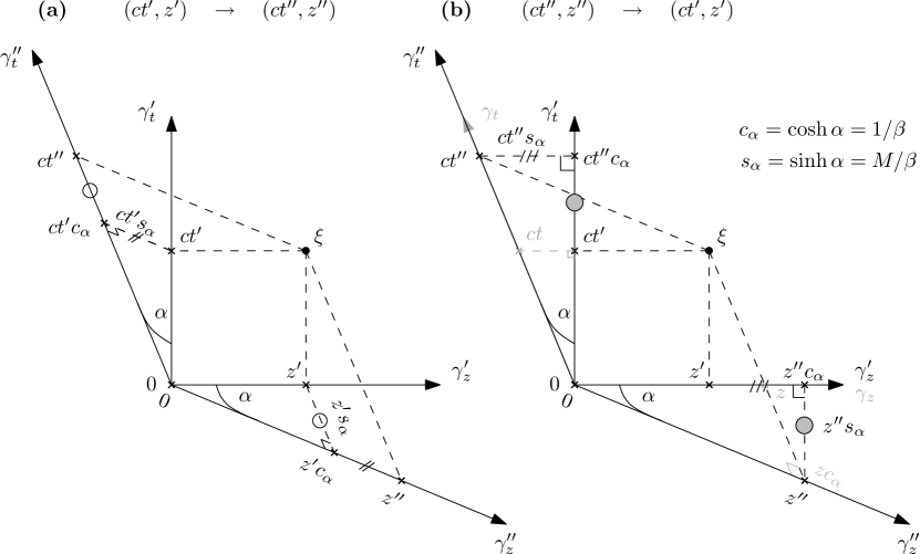
Figure 5: Geometric interpretation of the transformations between the fluid frame $\{\gamma^{\prime}_{\mu}\}$ and the Lorentzian frame $\{\gamma^{\prime\prime}_{\mu}\}$: (a) transformations from fluid coordinates $(ct^{\prime},z^{\prime})$ to Lorentzian coordinates $(ct^{\prime\prime},z^{\prime\prime})$; (b) transformations from Lorentzian coordinates $(ct^{\prime\prime},z^{\prime\prime})$ to fluid coordinates $(ct^{\prime},z^{\prime})$ and observer coordinates $(ct,z)$. The geometry of the fluid frame is Euclidean but the geometry of the Lorentzian frame is hyperbolic. In particular the angle $\alpha=\tanh^{-1}M$ is a hyperbolic angle. These two figures can be used to recover in a geometrical way the coordinate transformations between the observer frame, the fluid frame and the Lorentzian frame.

For example using the hyperbolic right angle triangles illustrated in Figure 5, we have,

$$ct^{\prime\prime}=ct^{\prime}\cosh\alpha+z^{\prime}\sinh\alpha=(1/\beta)(ct^{\prime}+Mz^{\prime})$$ (69)

$$z^{\prime\prime}=z^{\prime}\cosh\alpha+ct^{\prime}\sinh\alpha=(1/\beta)(z^{\prime}+Mct^{\prime}),$$ (70)

which corresponds to Eqn (22). Note that the right angle triangles look different from the usual Euclidean ones: the hypotenuse is shorter than the two other sides of the triangle, which is typical of hyperbolic geometry.

Similarly, one can invert the above transformations by projecting the Lorentzian coordinates onto the fluid frame, as illustrated in Figure 5,

$$ct^{\prime}=ct^{\prime\prime}\cosh\alpha-z^{\prime\prime}\sinh\alpha=(1/\beta)(ct^{\prime\prime}-Mz^{\prime\prime})$$ (71)

$$z^{\prime}=z^{\prime\prime}\cosh\alpha-ct^{\prime\prime}\sinh\alpha=(1/\beta)(z^{\prime\prime}-Mct^{\prime\prime}).$$ (72)

Using the same figure, one can readily express the Lorentzian coordinates in terms of the observer coordinates,

$$z^{\prime\prime}=z\cosh\alpha=z/\beta,$$ (73)

$$ct^{\prime}=(ct/\beta)\cosh\alpha=ct,\quad\text{so from Eqn~{}(\ref{eq:double-prime-to-prime-geometrically})}\quad ct^{\prime\prime}=\beta ct+Mz/\beta$$ (74)

which corresponds to Eqn (23).

Thus, the Lorentzian frame in which the wave equation retains its simplest form obeys the laws of hyperbolic geometry. This does not appear to have been fully appreciated in the aeroacoustics literature and may simplify future analyses.

4.4   The propagation operator $\mathcal{L}$ and the Laplacian in acoustic space-time

If we have an arbitrary frame $\{e_{i}\}$ $i=1,\ldots,n$ with reciprocal frame $\{e^{i}\}$, an arbitrary vector $\xi$ may be written,

$$\xi=x^{i}e_{i}\text{ where }x^{i}=\xi\cdot e^{i},$$ (75)

where the Einstein summation convention for repeated indices has been employed. For an arbitrary field $F(\xi)$, the vector derivative $\nabla$ is defined such that, for any vector $a$,

$$a\cdot\nabla F(\xi)=\lim_{\epsilon\rightarrow 0}\frac{F(\xi+\epsilon a)-F(\xi)}{\epsilon},$$ (76)

where we assume that the limit exists and is well defined. Note that $F$ can in general be any multivector field. It can be shown that the vector derivative can be written,

$$\nabla=\sum_{i=1}^{n}e^{i}\frac{\partial}{\partial x^{i}}=\sum_{i=1}^{n}e^{i}\partial_{x^{i}}.$$ (77)

This defines the shorthand $\partial_{x}$ for a partial derivative with respect to $x$. Note that $\nabla$ is frame independent.

Now let us consider the operator $\nabla\cdot\nabla$ in the acoustic space-time frames defined above. Using the definition in Eqn (77) $\nabla$ is given by,

$$\nabla =\gamma^{t}\partial_{ct}+\gamma^{x}\partial_{x}+\gamma^{y}\partial_{y}+\gamma^{z}\partial_{z}$$ (78)

$$={\gamma^{t}}^{\prime}\partial_{ct^{\prime}}+{\gamma^{x}}^{\prime}\partial_{x^{\prime}}+{\gamma^{y}}^{\prime}\partial_{y^{\prime}}+{\gamma^{z}}^{\prime}\partial_{z^{\prime}}$$

$$={\gamma^{t}}^{\prime\prime}\partial_{ct^{\prime\prime}}+{\gamma^{x}}^{\prime\prime}\partial_{x^{\prime\prime}}+{\gamma^{y}}^{\prime\prime}\partial_{y^{\prime\prime}}+{\gamma^{z}}^{\prime\prime}\partial_{z^{\prime\prime}}.$$

In all the frames defined the basis vectors do not vary over the space. Using this and the definitions of the basis vectors given above, we can show that,

$$\nabla\cdot\nabla =-\partial_{x}\partial_{x}-\partial_{y}\partial_{y}-\partial_{z}\partial_{z}+(\partial_{ct}+M\partial_{z})^{2}$$ (79)

$$=-\partial_{x^{\prime}}\partial_{x^{\prime}}-\partial_{y^{\prime}}\partial_{y^{\prime}}-\partial_{z^{\prime}}\partial_{z^{\prime}}+\partial_{ct^{\prime}}\partial_{ct^{\prime}}$$

$$=-\partial_{x^{\prime\prime}}\partial_{x^{\prime\prime}}-\partial_{y^{\prime\prime}}\partial_{y^{\prime\prime}}-\partial_{z^{\prime\prime}}\partial_{z^{\prime\prime}}+\partial_{ct^{\prime\prime}}\partial_{ct^{\prime\prime}}.$$

Hence it becomes clear that,

$$\mathcal{L}=-\nabla\cdot\nabla.$$ (80)

Our wave equation may therefore be written,

$$\nabla\cdot\nabla p(\xi)=f(\xi),$$ (81)

and depending on which frame we expand $\nabla\cdot\nabla$ in, we obtain either the convected or the un-convected wave equation. It is now clear why the Lorentz transform does not alter the form of $\mathcal{L}$. When the Lorentz transform acts on a frame that satisfies the simple space-time metric (Eqn (4)), the resulting frame also satisfies this metric, hence the expansion of $\mathcal{L}=-\nabla\cdot\nabla$ is not altered. However, when a Galilean transform is used, the resulting frame is no longer orthogonal, and this is why the expansion of $\nabla\cdot\nabla$ is more complex.

   onclusions

This paper presents a geometric framework to interpret the transformations used to solve the equation for sound propagation in uniform flow. By writing the wave operator in terms of the Laplacian of the acoustic space-time we are able to show clearly why the wave operator takes complex and simple forms in the different frames. The framework allows the transformation to be understood in terms of a combined Galilean and Lorentz transform. The Galilean transform simplifies the wave operator but moves us to a frame in motion with respect to the observer. The Lorentz transform takes us back to a frame that is stationary with respect to the observer, while keeping the wave operator simple. The use of Geometric algebra makes it clear that the Lorentz transform is really a generalised rotation.

The transformation derived in this way is used to give simple derivations of Green’s functions in the different frames. The geometric framework allows sound propagation to be understood in terms of the null vectors of the space, which are not dependent on the frame. A simple interpretation for transformations in frequency-wavenumber space in terms of the reciprocal frame is also provided, which is used to derive expressions for Doppler shifts.

We hope that this investigation will pave the way to more complex transformations applicable when the background flow is non-uniform. Here we have used a flat space-time to understand uniform flow transformation, and the natural extension would be to consider a curved acoustic space-time.

Appendix A The Reciprocal Frame

Here we follow [19]. Let us assume that we have a set of $n$ linearly independent vectors $\{\bm{e}_{k}\}$ that span an arbitrary $n$ dimensional space (arbitrary means that the frame can be Euclidean or hyperbolic, or indeed can have any metric). We refer to this set of $n$ vectors as our frame. Associated with any frame is a reciprocal frame of $n$ vectors, $\{\bm{e}^{k}\}$, defined by the property,

$$\bm{e}^{i}\cdot\bm{e}_{j}=\delta^{i}_{j},\quad\forall i,j=1,\ldots,n\qquad\delta^{i}_{j}=\left\{\begin{array}[]{ll}1&i=j\\ 0&i\neq j\end{array}\right..$$ (82)

A.1   Vector Components

The basis vectors $\{\bm{e}_{k}\}$ are linearly independent, so any vector $\bm{a}$ can be written uniquely in terms of this set as,

$$\bm{a}=\sum_{i=1}^{n}a^{i}\bm{e}_{i}=\sum_{i=1}^{n}a_{i}\bm{e}^{i}.$$ (83)

The set of scalars $(a^{1},\ldots,a^{n})$ are the components of the vector $\bm{a}$ in the $\{\bm{e}_{k}\}$ frame. To find these components we form,

$$\bm{a}\cdot\bm{e}^{i}=a^{j}\bm{e}_{j}\cdot\bm{e}^{i}=a^{j}\delta^{j}_{i}=a^{i},$$ (84)

$$\bm{a}\cdot\bm{e}_{i}=a_{j}\bm{e}^{j}\cdot\bm{e}_{i}=a_{j}\delta^{i}_{j}=a_{i}.$$ (85)

This derivation of how to find components explains the use of sub- and superscripts in Eqn (83). Note that if the frame is orthonormal, the frame and its reciprocal are equivalent.

A.2   Finding the Reciprocal Frame

Given that the basis vectors $\{\bm{e}_{k}\}$ are linearly independent, it must be possible to decompose every reciprocal vector as,

$$\bm{e}^{k}=a^{k}_{1}\bm{e}_{1}+\ldots+a^{k}_{n}\bm{e}_{n},$$ (86)

for some set of coefficients $a^{k}_{i}$. Given this and the requirement in Eqn (82), we can obtain a system of $n^{2}$ equations for the $n^{2}$ coefficients $a^{k}_{i}$. For large $n$ however, this will become rather cumbersome, and so we also present a result from geometric algebra that gives us an explicit expression for the reciprocal frame, which can be easily implemented in any symbolic algebra package.

We define the volume element for the $\{\bm{e}_{k}\}$ frame, $E_{n}$, as,

$$E_{n}=\bm{e}_{1}\wedge\bm{e}_{2}\wedge\cdots\wedge\bm{e}_{n}.$$ (87)

Note that $E_{n}$ is a multiple of the pseudoscalar $I$. We can construct the reciprocal frame as,

$$\bm{e}^{j}=(-1)^{j-1}\bm{e}_{1}\wedge\cdots\wedge\check{\bm{e}}_{j}\wedge\cdots\wedge\bm{e}_{n}\;E_{n}^{-1},$$ (88)

where the check on $\check{\bm{e}}_{j}$ denotes that this vector is excluded from the expression. We now justify this definition. $\bm{e}^{j}$ must be perpendicular to all the $\{\bm{e}_{i},i\neq j\}$, and hence we form the exterior product of these $n-1$ vectors, and then project onto the vector perpendicular to this $(n-1)$ volume element by multiplying by $E_{n}^{-1}$. The fact that we used $E_{n}^{-1}$ rather than $I$ ensures the correct normalisation. To prove this more formally we make use of the property of the pseudoscalar $I$, that for any vector $\bm{a}$ and multivector $A_{r}$ (of grade $r$) [19],

$$\bm{a}\cdot(A_{r}I)=(\bm{a}\wedge A_{r})I.$$ (89)

Let us define the scalar $C$ such that,

$$E_{n}=CI.$$ (90)

It follows that,

$$E_{n}^{-1}=\frac{1}{C}I^{-1},$$ (91)

and hence we can write,

$$\bm{e}_{i}\cdot\bm{e}^{j} =\frac{(-1)^{j-1}}{C}\bm{e}_{i}\cdot\left((\bm{e}_{1}\wedge\cdots\wedge\check{\bm{e}}_{j}\wedge\cdots\wedge\bm{e}_{n})I^{-1}\right)$$ (92)

$$=\frac{(-1)^{j-1}}{C}(\bm{e}_{i}\wedge\bm{e}_{1}\wedge\cdots\wedge\check{\bm{e}}_{j}\wedge\cdots\wedge\bm{e}_{n})I^{-1}.$$

If $i\neq j$ then this contains $\bm{e}_{i}\wedge\bm{e}_{i}$ and hence is zero. If $i=j$ we can write this as,

$$\bm{e}_{i}\cdot\bm{e}^{j} =\frac{1}{C}(\bm{e}_{1}\wedge\cdots\wedge\bm{e}_{j}\wedge\cdots\wedge\bm{e}_{n})I^{-1}$$ (93)

$$=\frac{1}{C}(CI)I^{-1}=1\text{ as required.}$$

Appendix B Spherical coordinates

• Observer coordinates $(R,\theta)$:

  $$R =R^{\prime}\sqrt{1+M^{2}+2M\cos\theta^{\prime}}=R^{\prime\prime}\sqrt{1-M^{2}\cos^{2}\theta^{\prime\prime}}$$ (94)

  $$\cos\theta =\frac{\cos\theta^{\prime}+M}{\sqrt{1+M^{2}+2M\cos\theta^{\prime}}}=\frac{\beta\cos\theta^{\prime\prime}}{\sqrt{1-M^{2}\cos^{2}\theta^{\prime\prime}}},$$ (95)

  $$\sin\theta =\frac{\sin\theta^{\prime}}{\sqrt{1+M^{2}+2M\cos\theta^{\prime}}}=\frac{\sin\theta^{\prime\prime}}{\sqrt{1-M^{2}\cos^{2}\theta^{\prime\prime}}};$$ (96)

• Lorentzian coordinates $(R^{\prime\prime},\theta^{\prime\prime})$:

  $$R^{\prime\prime} =\frac{R}{\beta}\sqrt{1-M^{2}\sin^{2}\theta}=\frac{R^{\prime}}{\beta}(1+M\cos\theta^{\prime}),$$ (97)

  $$\cos\theta^{\prime\prime} =\frac{\cos\theta}{\sqrt{1-M^{2}\sin^{2}\theta}}=\frac{M+\cos\theta^{\prime}}{1+M\cos\theta^{\prime}},$$ (98)

  $$\sin\theta^{\prime\prime} =\frac{\beta\sin\theta}{\sqrt{1-M^{2}\sin^{2}\theta}}=\frac{\beta\sin\theta^{\prime}}{1+M\cos\theta^{\prime}};$$ (99)

• Fluid coordinates $(R^{\prime},\theta^{\prime})$:

  $$R^{\prime} =\frac{R}{\beta^{2}}\left(\sqrt{1-M^{2}\sin^{2}\theta}-M\cos\theta\right)=\frac{R^{\prime\prime}}{\beta}\left(1-M\cos\theta^{\prime\prime}\right),$$ (100)

  $$\cos\theta^{\prime} =\frac{\cos\theta-M\sqrt{1-M^{2}\sin^{2}\theta}}{\sqrt{1-M^{2}\sin^{2}\theta}-M\cos\theta}=\frac{M-\cos\theta^{\prime\prime}}{M\cos\theta^{\prime\prime}-1},$$ (101)

  $$\sin\theta^{\prime} =\frac{\beta^{2}\sin\theta}{\sqrt{1-M^{2}\sin^{2}\theta}-M\cos\theta}=\frac{\beta\sin\theta^{\prime\prime}}{1-M\cos\theta^{\prime\prime}}.$$ (102)

It is interesting to note that the relationships involving the Lorentzian coordinates are more compact than those between the observer and fluid coordinates.

References

- Unruh [1981] Unruh, W. G. 1981 Experimental Black-Hole Evaporation? PRL, 46(21), 1351–1353.
- Visser [2013] Visser, M. 2013 Survey of analogue spacetimes. Lect. Notes Phys., 870, 31–50.
- Visser [1998] Visser, M. 1998 Acoustic black holes: horizons, ergospheres and Hawking radiation. Class. Quantum Grav., 15, 1767–1791.
- Barceló et al. [2004] Barceló, C., Liberati, S., Sonego, S. & Visser, M. 2004 Causal structure of acoustic spacetimes. New J. Phys., 6(1), 186.
- Leonhardt & Philbin [2009] Leonhardt, U. & Philbin, T. G. 2009 Transformation Optics and the Geometry of Light. Prog. Optics, 53, 69–152.
- Leonhardt [2006] Leonhardt, U. 2006 Optical Conformal Mapping. Science, 312(5781), 1777–1780.
- Zhang et al. [2011] Zhang, S., Xia, C. & Fang, N. 2011 Broadband Acoustic Cloak for Ultrasound Waves. PRL, 106(2), 024 301.
- Pendry & Li [2008] Pendry, J. B. & Li, J. 2008 An acoustic metafluid: realizing a broadband acoustic cloak. New J. Phys., 10(11), 115 032.
- Torrent & Sánchez-Dehesa [2008] Torrent, D. & Sánchez-Dehesa, J. 2008 Acoustic cloaking in two dimensions: a feasible approach. New J. Phys., 10(6), 063 015.
- Pendry et al. [2006] Pendry, J. B., Schurig, D. & Smith, D. R. 2006 Controlling Electromagnetic Fields. Science, 312(5781), 1780–1782.
- Leonhardt & Philbin [2006] Leonhardt, U. & Philbin, T. G. 2006 General relativity in electrical engineering. New J. Phys., 8(10), 247–247.
- Garrick & Watkins [1953] Garrick, I. E. & Watkins, C. E. 1953 A theoretical study of the effect of forward speed on the free-space sound-pressure field around propellers. Tech. Rep. NACA TN 3018.
- Bateman [1917] Bateman, H. 1917 Döppler’s principle for a windy atmosphere. Mon. Weather Rev., 45(9), 441–442.
- Gerkema et al. [2013] Gerkema, T., Maas, L. R. M. & van Haren, H. 2013 A Note on the Role of Mean Flows in Doppler-Shifted Frequencies. J. Phys. Oceanogr., 43(2), 432–441.
- Hestenes [2003] Hestenes, D. 2003 Oersted Medal Lecture 2002: Reforming the Mathematical Language of Physics. Am. J. Phys., 71(2), 104–121.
- Hestenes [1992] Hestenes, D. 1992 Space-time algebra. Gordon & Breach Science Pub.
- Clifford [1878] Clifford, W. K. 1878 Applications of Grassmann’s Extensive Algebra. Am. J. Math., 1(4), 350–358.
- Grassmann [1844] Grassmann, H. 1844 Die lineale Ausdehnungslhre ein neuer Zweig der Mathematik. Leipzig: Verlag von Otto Wigand.
- Doran & Lasenby [2003] Doran, C. J. L. & Lasenby, A. N. 2003 Geometric Algebra for Physicists. Cambridge: Cambridge University Press.
- Arthur [2011] Arthur, J. W. 2011 Understanding Geometric Algebra for Electromagnetic Theory. Checester: John Wiley and Sons.
- Abbott et al. [2010] Abbott, D., Chappell, J. M. & Iqbal, A. 2010 A simplified approach to electromagnetism using geometric algebra. arXiv.
- Zou et al. [2011] Zou, L., Lasenby, J. & He, Z. 2011 Beamforming with distortionless co-polarisation for conformal arrays based on geometric algebra. IET Radar Sonar Navig., 5(8), 842–853.
- Jones [1989] Jones, D. S. 1989 Acoustic and Electromagnetic Waves. Oxford University Press.
- Carcione & Cavallini [1995] Carcione, J. M. & Cavallini, F. 1995 On the acoustic-electromagnetic analogy. Wave Motion, 21(2), 149–162.
- Doran et al. [2002] Doran, C. J. L., Dorst, L. & Lasenby, J. 2002 Applications of Geometric Algebra in Computer Science and Engineering. Springer.
- McRobie & Lasenby [1999] McRobie, F. A. & Lasenby, J. 1999 Simo-Vu Quoc Rods Using Clifford Algebra. Int. J. Numer. Meth. Eng., 45, 377–398.
- Stratton [1941] Stratton, J. A. 1941 Electromagnetic Theory. New York: McGraw Hill.
- Lighthill [1962] Lighthill, M. J. 1962 The Bakerian Lecture, 1961. Sound Generated Aerodynamically. Proc. R. Soc. Lond. A, 267(1329), 147–182.
- Dowling & Ffowcs Williams [1983] Dowling, A. P. & Ffowcs Williams, J. E. 1983 Sound and Sources of Sound. Chichester: Ellis Horwood Limited.
- Rienstra & Hirschberg [2013] Rienstra, S. W. & Hirschberg, A. 2013 An Introduction to Acoustics. Report IWDE.
- Joseph et al. [1998] Joseph, P. F., Morfey, C. L. & Nelson, P. A. 1998 Active control of source sound power radiation in uniform flow. J. Sound Vib., 212(2), 357–364.
- Chapman [1994] Chapman, C. J. 1994 Sound radiation from a cylindrical duct. Part 1. Ray structure of the duct modes and of the external field. J. Fluid Mech., 281, 293–311.
- Joseph et al. [2010] Joseph, P. F., Sinayoko, S. & McAlpine, A. 2010 Multimode radiation from an unflanged, semi-infinite circular duct with uniform flow. J. Acoust. Soc. Am., 127(4), 2159.
- Amiet [1976] Amiet, R. K. 1976 High frequency thin-airfoil theory for subsonic flow. AIAA J., 14(8), 1076–1082.
- Roger & Moreau [2005] Roger, M. & Moreau, S. 2005 Back-scattering correction and further extensions of Amiet’s trailing-edge noise model. Part 1: theory. J. Sound Vib., 286, 477–506.
- Küssner [1940] Küssner, H. G. 1940 General Airfoil Theory. Luftfahrtforschung, 17(11/12), 1–29.
- Graham [1970] Graham, J. M. R. 1970 Similarity rules for thin aerofoils in non-stationary subsonic flows. J. Fluid Mech., 43(04), 753–766.
- Chapman [2000] Chapman, C. J. 2000 Similarity Variables for Sound Radiation in a Uniform Flow. J. Sound Vib., 233(1), 157–164.
- Blandeau & Joseph [2011] Blandeau, V. P. & Joseph, P. F. 2011 Validity of Amiet’s Model for Propeller Trailing-Edge Noise. AIAA J., 49(5), 1057–1066.
- Sinayoko et al. [2013] Sinayoko, S., Kingan, M. & Agarwal, A. 2013 Trailing edge noise theory for rotating blades in uniform flow. Proc. R. Soc. Lond. A, 469(2157), 20130 065.
- Pierce [1981] Pierce, A. D. 1981 Acoustics, An Introduction to its Physical Principles and Applications. The Acoustical Society of America.
- Martinez & Widnall [1980] Martinez, R. & Widnall, S. E. 1980 Unified aerodynamic-acoustic theory for a thin rectangular wing encountering a gust. AIAA J., 18(6), 636–645.
- Martinez & Widnall [1983] Martinez, R. & Widnall, S. E. 1983 An aeroacoustic model for high-speed, unsteady blade-vortex interaction. AIAA J., 21(9), 1225–1231.
- Hanson [1995] Hanson, D. B. 1995 Sound from a Propeller at Angle of Attack: A New Theoretical Viewpoint. Proc. R. Soc. Lond. A, 449(1936), 315–328.
- Crighton et al. [1992] Crighton, D. G., Dowling, A. P., Ffowcs Williams, J. E., Heckl, M. & Leppington, F. G. 1992 Modern Methods in Analytical Acoustics. London: Springer.
- Morse & Feshbach [1953] Morse, P. M. & Feshbach, H. 1953 Methods of Theoretical Physics, Part II. Chapters 9 to 13. McGraw Hill.
- Rozenberg et al. [2010] Rozenberg, Y., Roger, M. & Moreau, S. 2010 Rotating Blade Trailing-Edge Noise: Experimental Validation of Analytical Model. AIAA J., 48(5), 951–962.
- Lasenby et al. [2000] Lasenby, J., Lasenby, A. N. & Doran, C. J. L. 2000 A unified mathematical language for physics and engineering in the 21st century. Phil. Trans. R. Soc. Lond. A, 358(1765), 21–39.
- Cibura & Hildenbrand [2008] Cibura, C. & Hildenbrand, D. 2008 Geometric Algebra Approach to Fluid Dynamics. Tech. rep., Technische Universität Darmstadt, Amsterdam.