Cosmological solutions and observational constraints on 5-dimensional braneworld cosmology with gravitating Nambu-Goto matching conditions

Abstract

We investigate the cosmological implications of the recently constructed 5-dimensional braneworld cosmology with gravitating Nambu-Goto matching conditions. Inserting both matter and radiation sectors, we extract analytical cosmological solutions. Additionally, we use observational data from Type Ia Supernovae (SNIa) and Baryon Acoustic Oscillations (BAO), along with requirements of Big Bang Nucleosynthesis (BBN) and Cosmic Microwave Background (CMB) radiation, in order to impose constraints on the parameters of the model. We find that the scenario at hand is in good agreement with observations, and thus a small departure from the standard Randall-Sundrum scenario is allowed. However, the concordance $\Lambda$CDM cosmology is still favored comparing to both standard braneworld model and the present scenario.

1 Introduction

Israel matching conditions [1] are considered as the standard equations of motion of a classical codimension-1 defect which backreacts on the bulk dynamics. They are derived by focusing on the distributional part of the Einstein field equations (or some gravity modification) where the brane energy-momentum tensor, specified by a delta function, is included. An equivalent way to derive these equations is to take the variation of the brane-bulk action with respect to the induced metric, while the bulk equations of motion are derived as usually by varying the bulk action with respect to the bulk metric. However, a higher codimension defect carrying a generic energy-momentum tensor is known to be inconsistent with Einstein’s equations [2, 3, 4] (a brane with a pure tension is a special consistent case [5, 6, 7, 8, 9, 10, 11, 12, 13]). In [14] it was considered the idea that a more general theory like Einstein-Gauss-Bonnet gravity in six dimensions might remove the previous inconsistency, and the matching conditions of the theory for a generic energy-momentum tensor were derived. In [15] the consistency of the whole system of bulk field equations plus matching conditions was shown for an axially symmetric codimension-2 cosmological brane.

The spirit of the above proposal for consistency of the higher codimension defects is to include higher Lovelock densities [17, 18]. However, in $D$ dimensions, the highest such density is of order $[(D-1)/2]$, and so, it is quite probable that branes with codimension higher than $[(D-1)/2]$ will still be inconsistent. Moreover, four-dimensions which represent effectively spacetime at certain length and energy scales do not allow generic codimension-2 or 3 defects. On the other hand, Israel matching conditions and their generalizations to higher codimensions do not accept the Nambu-Goto probe limit, which is the lowest order approximation of a test brane moving in curved background. Even the geodesic limit of the Israel matching conditions is questionable as a probe limit, since being the geodesic equation a kinematical fact it should be preserved independent of the gravitational theory (similarly to [19], [20]) or the codimension of the defect, which is not the case for these matching conditions [14, 21, 22, 23, 24, 25]. Moreover, even the non-geodesic probe limit of the standard equations of motion for various codimension defects in Lovelock gravity theories is not accepted, since this consists of higher order algebraic equations in the extrinsic curvature, and therefore, a multiplicity of probe solutions arise instead of a unique equation of motion at the probe level. In view of these observations a criticism to the standard matching conditions appeared in [16], where alternative matching conditions were proposed. These are the “gravitating Nambu-Goto matching conditions” which arise by the variation of the brane-bulk action with respect to the brane embedding fields, so that the gravitational back-reaction of the brane is taken into account. With these matching conditions a brane is always consistent for an arbitrary energy-momentum tensor and it also possesses the Nambu-Goto probe limit (the codimension-2 case was studied in [16], [26], while the codimension-1 in [27]). In [27] the application of these alternative matching conditions led to a new 5-dimensional braneworld cosmology which generalizes the conventional braneworld cosmology [28] in the sense that it contains an extra integration constant, and vanishing this constant gives back the standard braneworld cosmology.

In the current work we try to confront this cosmology with the current cosmological observational data (SNIa, BAO, BBN) in order to construct the corresponding probability contour-plots for the parameters of the theory. The paper is organized as follows: In section 2 we briefly present the alternative matching conditions and the basic features behind these, and we find in the cosmological framework the equation for the expansion rate including both the matter and radiation sectors. In section 3, which is the main part of the work, we impose the observational constraints on the parameters of the model. Finally, a summary of the obtained results is given in section 4 of conclusions.

2 5-dimensional braneworld with gravitating Nambu-Goto matching conditions

Our system is described by five-dimensional Einstein gravity coupled to a localized 3-brane source. The domain wall $\Sigma$ is assumed to be $Z_{2}-$symmetric, it splits the spacetime $\mathcal{M}$ into two parts $\mathcal{M}_{\pm}$ and the two sides of $\Sigma$ are denoted by $\Sigma_{\pm}$. The total brane-bulk action is

$$\!\!\!\!\!S=\int_{\mathcal{M}}d^{5}x\sqrt{|\textsl{g}|}\,\big{(}M^{3}\mathcal{R}-\Lambda\big{)}-V\int_{\Sigma}d^{4}\chi\sqrt{|h|}-2M^{3}\int_{\Sigma_{\pm}}\!\!d^{4}\chi\sqrt{|h|}\,K+\int_{\Sigma}d^{4}\chi\,L_{mat}\,,$$ (2.1)

where $\textsl{g}_{\mu\nu}$ is the (continuous) bulk metric tensor and $h_{\mu\nu}=\textsl{g}_{\mu\nu}-n_{\mu}n_{\nu}$ is the induced metric on the brane with $n^{\mu}$ the unit normals pointing inwards $\mathcal{M}_{\pm}$ ($\mu,\nu,...$ are five-dimensional coordinate indices). The bulk coordinates are $x^{\mu}$ and the brane coordinates are $\chi^{i}$ ($i,j,...$ are coordinate indices on the brane). The brane tension is $V>0$ and the matter Lagrangian of the brane is $L_{mat}$. The only matter content of the bulk is the cosmological constant $\Lambda<0$ and the higher dimensional mass scale is $M$. The contribution on each side of the wall of the Gibbons-Hawking term is also necessary here as in the standard derivation of the matching conditions. $K=h^{\mu\nu}K_{\mu\nu}$ is the trace of the extrinsic curvature $K_{\mu\nu}=h^{\kappa}_{\mu}h^{\lambda}_{\nu}n_{\kappa;\lambda}$ (the covariant differentiation ; corresponds to $\textsl{g}_{\mu\nu}$).

Varying (2.1) with respect to the bulk metric we get the bulk equations of motion

$$\mathcal{G}_{\mu\nu}=-\frac{\Lambda}{2M^{3}}\textsl{g}_{\mu\nu}\,,$$ (2.2)

where $\mathcal{G}_{\mu\nu}$ is the bulk Einstein tensor. In this variation, beyond the basic terms proportional to $\delta\textsl{g}_{\mu\nu}$ which give (2.2), there appear, as usually, extra terms proportional to the second covariant derivatives $(\delta\textsl{g}_{\mu\nu})_{;\kappa\lambda}$ which lead to a surface integral on the brane with terms proportional to $(\delta\textsl{g}_{\mu\nu})_{;\kappa}$. Adding the Gibbons-Hawking term, the normal derivatives of $\delta\textsl{g}_{\mu\nu}$, i.e. terms of the form $n^{\kappa}(\delta\textsl{g}_{\mu\nu})_{;\kappa}$, are canceled, and considering as boundary condition for the variation of the bulk metric its vanishing on the brane (Dirichlet boundary condition for $\delta\textsl{g}_{\mu\nu}$) there is nothing left beyond the terms in equation (2.2). The Gibbons-Hawking term will again contribute in the following variation performed in order to obtain the brane equations of motion.

According to the standard method, the interaction of the brane with the bulk comes from the variation $\delta\textsl{g}_{\mu\nu}$ at the brane position of the action (2.1), which is equivalent to adding on the right-hand side of equation (2.2) the term $\kappa_{5}^{2}\,\tilde{T}_{\mu\nu}\,\delta^{(1)}$, where $\tilde{T}_{\mu\nu}=\sqrt{|h|/|\textsl{g}|}\,\big{(}T_{\mu\nu}-\lambda\,h_{\mu\nu}\big{)}$, $T_{\mu\nu}$ is the brane energy-momentum tensor and $\delta^{(1)}$ is the one-dimensional delta function with support on the defect. This approach leads to the standard Israel matching conditions. Here, we discuss an alternative approach where the interaction of the brane with bulk gravity is obtained by varying the total action (2.1) with respect to $\delta x^{\mu}$, the embedding fields of the brane position [16]. The embedding fields are some functions $x^{\mu}(\chi^{i})$ and their variations are $\delta x^{\mu}(x^{\nu})$. While in the standard method the variation of the bulk metric at the brane position remains arbitrary, here the corresponding variation is induced by $\delta x^{\mu}$, i.e. $\delta\textsl{g}_{\mu\nu}=-\pounds_{\delta x}\textsl{g}_{\mu\nu}$. The result of this variation gives the codimension-1 gravitating Nambu-Goto matching conditions [27] (for a reminiscent variation see also [30])

$$\Big{[}K^{ij}-Kh^{ij}+\frac{1}{4M^{3}}(T^{ij}-Vh^{ij})\Big{]}K_{ij}=0$$ (2.3)

$$T^{ij}_{\,\,\,\,|j}=-4M^{3}\big{(}K^{ij}-Kh^{ij}\big{)}_{|j}\,,$$ (2.4)

where $K_{ij}=K_{ij}^{+}=K_{ij}^{-}$, $K^{\mu\nu}=K^{ij}x^{\mu}_{\,\,,i}x^{\nu}_{\,\,,j}$ and $|$ denotes covariant differentiation with respect to $h_{\mu\nu}$. These equations are supplemented with the bulk equations (2.2) which are defined limitingly on the brane, and therefore, additional equations have to be satisfied at the brane position beyond the matching conditions. Using these bulk equations the system of the above matching conditions (2.3), (2.4) is written equivalently as

$$\big{(}T^{ij}-Vh^{ij}\big{)}K_{ij}=4(M^{3}R-\Lambda)$$ (2.5)

$$T^{ij}_{\,\,\,\,|j}=0\,,$$ (2.6)

where $R$ is the 3-dimensional Ricci scalar.

In order to search for cosmological solutions we consider the corresponding form for the bulk metric in the Gaussian-normal coordinates

$$ds_{5}^{2}=dy^{2}-n^{2}(t,y)dt^{2}+a^{2}(t,y)\,\gamma_{\hat{i}\hat{j}}(\chi^{\hat{\ell}})d\chi^{\hat{i}}d\chi^{\hat{j}}\,,$$ (2.7)

where $\gamma_{\hat{i}\hat{j}}$ is a maximally symmetric 3-dimensional metric ($\hat{i},\hat{j},...=1,2,3$) characterized by its spatial curvature $k=-1,0,1$. The energy-momentum tensor on the brane $T_{ij}$ (beyond that of the brane tension $V$) is assumed to be the one of perfect cosmic fluids with total energy density $\rho$ and total pressure $p$.

The $ty$, $yy$ bulk equations (2.2) at the position of the brane are

$$\dot{A}+nH(A-N)=0$$ (2.8)

$$A(A+N)-(X+Y)+\frac{\Lambda}{6M^{3}}=0\,,$$ (2.9)

where

$$A=\frac{a^{\prime}}{a}\ ,\ \ N=\frac{n^{\prime}}{n},$$

$$H=\frac{\dot{a}}{na}\,,$$

$$X=H^{2}+\frac{k}{a^{2}}\,,$$

$$Y=\frac{\dot{H}}{n}+H^{2}=\frac{\dot{X}}{2nH}+X\,,$$ (2.10)

and a prime, a dot denote respectively $\partial/\partial{y}$, $\partial/\partial{t}$. The cosmic scale factor, lapse function and Hubble parameter arise as the restrictions on the brane of the functions $a(t,y),n(t,y)$ and $H(t,y)$ respectively. Other quantities also have their corresponding values when restricted on the brane, and since all the following equations will refer to the brane position, we will use the same symbols for the restricted quantities without confusion. Combining equations (2.8), (2.9) together with the matching condition (2.5) [27], we obtain the solution for $A$

$$A=\pm\sqrt{X-\frac{\mathcal{C}}{a^{4}}-\frac{\Lambda}{12M^{3}}}\,\,,$$ (2.11)

where $\mathcal{C}$ is integration constant, and the Raychaudhuri equation for the brane cosmology

$$\frac{\dot{H}}{n}+2H^{2}+\frac{k}{a^{2}}-\frac{\Lambda}{6M^{3}}=\frac{\rho+3p-2V}{4M^{3}}\,\frac{H^{2}+\frac{k}{a^{2}}-\frac{\mathcal{C}}{a^{4}}-\frac{\Lambda}{12M^{3}}}{\frac{\rho+V}{4M^{3}}\pm 6\sqrt{H^{2}+\frac{k}{a^{2}}-\frac{\mathcal{C}}{a^{4}}-\frac{\Lambda}{12M^{3}}}}\,.$$ (2.12)

It is seen from (2.12) that for $\mathcal{C}=k=\rho=p=0$, the lower branch contains the Minkowski solution under the assumption of the Randall-Sundrum fine-tuning $\Lambda+V^{2}/(12M^{3})=0$ [31, 32]. We will not assume this condition in our analysis, so in the absence of matter our cosmology may have a de-Sitter vacuum. It is assumed that the quantity inside the square root of equation (2.12) is positive.

In [27] a single component perfect fluid was considered. Here, since we want to confront the model with real data, we will be more precise by assuming that the total energy density $\rho$ consists of the matter component $\rho_{m}$ with $p_{m}=0$ and the radiation component $\rho_{r}$ with $p_{r}=\frac{1}{3}\rho_{r}$, i.e. $\rho=\rho_{m}+\rho_{r}$. Now, the integration process of (2.12) differs from that in [27]. The variable

$$\Xi=\frac{1}{2}\ln{\Big{[}\frac{12M^{3}}{-\Lambda}\Big{(}H^{2}+\frac{k}{a^{2}}-\frac{\mathcal{C}}{a^{4}}-\frac{\Lambda}{12M^{3}}\Big{)}\Big{]}}$$ (2.13)

obeys the differential equation

$$\frac{d\Xi}{d\ln{a}}=\frac{\tilde{\rho}+3\tilde{p}}{\tilde{\rho}\pm 6e^{\Xi}}-2\,,$$ (2.14)

where

$$\tilde{\rho}=\sqrt{\frac{12M^{3}}{-\Lambda}}\,\frac{\rho+V}{4M^{3}}=\frac{\rho}{\rho_{\ast}}+\tilde{V}$$ (2.15)

$$\tilde{p}=\sqrt{\frac{12M^{3}}{-\Lambda}}\,\frac{p-V}{4M^{3}}=\frac{p}{\rho_{\ast}}-\tilde{V}$$ (2.16)

$$\tilde{V}=\frac{V}{\rho_{\ast}}$$ (2.17)

$$\rho_{\ast}=4M^{3}\sqrt{\frac{-\Lambda}{12M^{3}}}\,\,.$$ (2.18)

Note that the Randall-Sundrum fine-tuning corresponds to the value $\tilde{V}=3$. Using the conservation equation (2.6) in the standard form

$$\dot{\rho}+3nH(\rho+p)=0\,,$$ (2.19)

we obtain the equation

$$\frac{d\tilde{\rho}}{d\ln{a}}+3(\tilde{\rho}+\tilde{p})=0\,.$$ (2.20)

Finally, changing to the variable

$$\Phi=(\tilde{\rho}\pm 6e^{\Xi})^{2}\,,$$ (2.21)

we get from (2.14), (2.20), after some cancelations, the differential equation

$$\frac{d\Phi}{d\ln{a}}+4\Phi=-2\tilde{\rho}(\tilde{\rho}+3\tilde{p})\,.$$ (2.22)

Each fluid component is conserved independently

$$\dot{\rho}_{m}+3nH(\rho_{m}+p_{m)}=0\quad,\quad\dot{\rho}_{r}+3nH(\rho_{r}+p_{r})=0\,,$$ (2.23)

so the solutions are

$$\rho_{m}=\frac{\rho_{m0}}{a^{3}}\quad,\quad\rho_{r}=\frac{\rho_{r0}}{a^{4}}\,.$$ (2.24)

Therefore, equation (2.22) becomes a linear differential equation in terms of $a$

$$\frac{d\Phi}{d\ln{a}}+4\Phi=-\frac{2}{\rho_{\ast}^{2}}\Big{(}\frac{\rho_{m0}}{a^{3}}+\frac{\rho_{r0}}{a^{4}}+V\Big{)}\Big{(}\frac{\rho_{m0}}{a^{3}}+2\frac{\rho_{r0}}{a^{4}}-2V\Big{)}\,,$$ (2.25)

with general solution

$$\Phi=\frac{1}{\rho_{\ast}^{2}}\big{[}\big{(}\rho_{m}+\rho_{r}+V\big{)}^{2}-2V\rho_{r}\big{]}+\frac{\tilde{c}}{a^{4}}\,,$$ (2.26)

where $\tilde{c}$ is integration constant.

From the definition (2.21) we can find that

$$\tilde{\rho}\pm\frac{24M^{3}}{\rho_{\ast}}\sqrt{H^{2}+\frac{k}{a^{2}}-\frac{\mathcal{C}}{a^{4}}-\frac{\Lambda}{12M^{3}}}=\epsilon\,\sqrt{\Phi}\,.$$ (2.27)

In this equation the sign index $\epsilon=+1$ or $-1$ has been used to denote a new different bifurcation from the previous $\pm$ branches. It is seen from (2.27) that the sign $\epsilon=-1$ is only consistent with the lower $\pm$ branch, while the sign $\epsilon=+1$ is consistent with both $\pm$ branches. The distinction, however, introduced by the sign index $\pm$ will be lost in the expressions for the expansion rate and the acceleration parameter and only the sign $\epsilon$ will distinguish the two branches of solutions.
The expansion rate of the new cosmology arises by squaring equation (2.27) and is given by

$$H^{2}+\frac{k}{a^{2}}-\frac{\mathcal{C}}{a^{4}}=\Big{(}\frac{\rho_{\ast}}{24M^{3}}\Big{)}^{2}\,\Bigg{\{}\Bigg{[}\frac{\rho_{m}+\rho_{r}}{\rho_{\ast}}+\tilde{V}-\epsilon\ \sqrt{\Big{(}\frac{\rho_{m}+\rho_{r}}{\rho_{\ast}}+\tilde{V}\Big{)}^{2}-2\tilde{V}\frac{\rho_{r}}{\rho_{\ast}}+\frac{\tilde{c}}{a^{4}}}\,\Bigg{]}^{2}-36\Bigg{\}},$$ (2.28)

where in (2.28) one can set $\rho_{r}=0$. Redefining the integration constant $\tilde{c}$ as $\textsf{c}=\frac{\rho_{\ast}}{\rho_{r0}}\tilde{c}-2\tilde{V}$, the expansion rate can also be written as

$$H^{2}+\frac{k}{a^{2}}-\frac{\mathcal{C}}{a^{4}}=\Big{(}\frac{\rho_{\ast}}{24M^{3}}\Big{)}^{2}\,\Bigg{\{}\Bigg{[}\frac{\rho_{m}+\rho_{r}}{\rho_{\ast}}+\tilde{V}-\epsilon\,\sqrt{\Big{(}\frac{\rho_{m}+\rho_{r}}{\rho_{\ast}}+\tilde{V}\Big{)}^{2}+\textsf{c}\frac{\rho_{r}}{\rho_{\ast}}}\,\Bigg{]}^{2}-36\Bigg{\}},$$ (2.29)

where in (2.29) one cannot set $\rho_{r}=0$ since $\rho_{r0}$ is in the denominator of the definition of c. This solution contains two integrations constants. The first constant $\mathcal{C}$ is associated with the usual dark radiation term reflecting the non-vanishing bulk Weyl tensor. The second constant $\tilde{c}$ or c is the new feature that does not appear in the cosmology of the standard matching conditions [28] and signals new characteristics in the cosmic evolution. Setting $\textsf{c}=0\Leftrightarrow\tilde{c}=\frac{2\tilde{V}\rho_{r0}}{\rho_{\ast}}$ in the branch $\epsilon=-1$ we obtain the braneworld cosmology of the standard matching conditions $H^{2}+\frac{k}{a^{2}}-\frac{\mathcal{C}}{a^{4}}=\big{(}\frac{\rho_{m}+\rho_{r}+V}{12M^{3}}\big{)}^{2}+\frac{\Lambda}{12M^{3}}$ (if there is no radiation we just set $\tilde{c}=0$). Of course, there are always the extra integration constants $\rho_{m0}$, $\rho_{r0}$ of equations (2.24) which are adjusted by the today matter contents, while the today Hubble value $H_{0}$ is assumed to be given. The solution also contains three free parameters $M$, $V$, $\Lambda$ or $M$, $\tilde{V}$, $\rho_{\ast}$. In [27] for a single dust perfect fluid, which approximates well at least the late-times behaviour, it was found analytically for values of $\tilde{V}$ extremely close to the Randall-Sundrum fine-tuning the position of the recent passage from a long deceleration era to the present accelerating epoch. Moreover, the age of the universe was estimated and the time variability of the dark energy equation of state was calculated.

3 Observational constraints

As we analyzed in detail above, the cosmological scenario at hand leads to the Friedmann equation (2.28), where the index $\epsilon=\pm 1$ corresponds to two branches of solutions. The Friedmann equation contains the following parameters: $\mathcal{C}$, $\tilde{c}$, $M$, $\tilde{V}$ and $\rho_{\ast}$, along with $\Omega_{m0}$, $\Omega_{r0}$, $\Omega_{k0}$. $\mathcal{C}$ and $\tilde{c}$ are integration constants, $M$ is the fundamental 5D Planck mass, and the other two $\tilde{V}$, $\rho_{\ast}$ are connected to the fundamental model parameters $M$, $V$ and $\Lambda$ through the relations (2.17), (2.18). The identification of Newton’s constant $G_{N}$ in equation (2.28) as a combination of the model parameters will reduce the number of these parameters by one. Then, using $G_{N}$ we will define the various density parameters.

3.1 Branch $\epsilon=-1$

The scale factor for the branch $\epsilon=-1$ with $\tilde{V}<3$ is bounded from above and we will not consider this case in detail. However, the branch $\epsilon=-1$ with $\tilde{V}\geq 3$ possesses the late-times asymptotic linearized regime (that is when $\rho_{m}+\rho_{r}<<\rho_{\ast}\tilde{V}$, $\rho_{r}/\rho_{r0}<<\tilde{V}^{2}/\tilde{c}$) with a positive effective cosmological constant

$$H^{2}+\frac{k}{a^{2}}\approx\frac{\Lambda_{eff}}{3}+2\gamma\rho_{m}+\gamma\rho_{r}+\Big{(}\mathcal{C}+\frac{\gamma\rho_{\ast}\tilde{c}}{2\tilde{V}}\Big{)}\frac{1}{a^{4}}\,,$$ (3.1)

where

$$\gamma=\frac{V}{144M^{6}}$$ (3.2)

$$\Lambda_{eff}=3{\Big{(}{\frac{\rho_{\ast}}{4{M^{3}}}}\Big{)}^{2}}\,\Big{(}{\frac{\tilde{V}^{2}}{9}-1}\Big{)}=\frac{1}{4M^{3}}\Big{(}{\Lambda+\frac{V^{2}}{12M^{3}}}\Big{)}.$$ (3.3)

Now, as usual in braneworld or other modified gravity models, from this late-times Friedmann equation, one reads the Newton’s constant. Since asymptotically the coefficients of $\rho_{m},\rho_{r}$ in (3.1) are different, and $\rho_{r}\ll\rho_{m}$, we associate Newton’s constant with $\rho_{m}$

$$\gamma=\frac{V}{144M^{6}}\equiv\frac{4\pi G_{N}}{3}.$$ (3.4)

With this identification we can go back to the full Friedmann equation (2.28) and reduce one parameter, for instance $M$. Thus, the expansion rate (2.28) for $\epsilon=-1$, $\tilde{V}\geq 3$ becomes

$$H^{2}+\frac{k}{a^{2}}-\frac{\mathcal{C}}{a^{4}}=\frac{\pi G_{N}\rho_{\ast}}{3\tilde{V}}\,\Bigg{\{}\Bigg{[}\frac{\rho_{m}+\rho_{r}}{\rho_{\ast}}+\tilde{V}+\sqrt{\Big{(}\frac{\rho_{m}+\rho_{r}}{\rho_{\ast}}+\tilde{V}\Big{)}^{2}-2\tilde{V}\frac{\rho_{r}}{\rho_{\ast}}+\frac{\tilde{c}}{a^{4}}}\,\Bigg{]}^{2}-36\Bigg{\}}\,.$$ (3.5)

Finally, in order to complete the steps we rewrite (3.5) as

$$H^{2}+\frac{k}{a^{2}}-\frac{\mathcal{C}}{a^{4}}=\frac{8\pi G_{N}}{3}(\rho_{m}+\rho_{r}+\rho_{DE})$$ (3.6)

with

$$\rho_{DE}=\frac{\rho_{\ast}}{8\tilde{V}}\,\Bigg{\{}\Bigg{[}\frac{\rho_{m}+\rho_{r}}{\rho_{\ast}}+\tilde{V}+\sqrt{\Big{(}\frac{\rho_{m}+\rho_{r}}{\rho_{\ast}}+\tilde{V}\Big{)}^{2}-2\tilde{V}\frac{\rho_{r}}{\rho_{\ast}}+\frac{\tilde{c}}{a^{4}}}\,\Bigg{]}^{2}-36\Bigg{\}}-(\rho_{m}+\rho_{r})\,.$$ (3.7)

Note that this $\rho_{DE}$ at late-times goes to $\frac{\Lambda_{eff}}{8\pi G_{N}}-\frac{\rho_{r}}{2}+\frac{\rho_{\ast}\tilde{c}}{4\tilde{V}a^{4}}$ which asymptotically goes to $\frac{\Lambda_{eff}}{8\pi G_{N}}$, i.e. to a simple cosmological constant.

So now, we can define the various density parameters straightforwardly as

$$\Omega_{m}=\frac{8\pi G_{N}\rho_{m}}{3H^{2}}$$ (3.8)

$$\Omega_{r}=\frac{8\pi G_{N}\rho_{r}}{3H^{2}}$$ (3.9)

$$\Omega_{DE}=\frac{8\pi G_{N}\rho_{DE}}{3H^{2}}$$ (3.10)

$$\Omega_{k}=-\frac{k}{a^{2}H^{2}}$$ (3.11)

$$\Omega_{\mathcal{C}}=\frac{\mathcal{C}}{a^{4}H^{2}}.$$ (3.12)

Finally, assuming that the present scale factor is $a_{0}=1$ and using the redshift as the independent variable ($1/a=1+z$), we can write the Friedmann equation (3.6) in the usual form, convenient to observational fittings

$$\!\!\!H^{2}=H_{0}^{2}\left\{\Omega_{k0}(1\!+\!z)^{2}+\Omega_{\mathcal{C}0}(1\!+\!z)^{4}+\Omega_{m0}(1\!+\!z)^{3}+\Omega_{r0}(1\!+\!z)^{4}+\frac{8\pi G_{N}\rho_{DE}(z)}{3H_{0}^{2}}\right\}\,.$$ (3.13)

Here, $\rho_{DE}$, according to (3.7), is

$$\rho_{DE}(z) = \frac{\rho_{\ast}}{8\tilde{V}}\,\Bigg{\{}\left[\frac{3H_{0}^{2}\Omega_{m0}}{8\pi G_{N}\rho_{\ast}}(1+z)^{3}+\frac{3H_{0}^{2}\Omega_{r0}}{8\pi G_{N}\rho_{\ast}}(1+z)^{4}+\tilde{V}+\mathcal{A}(z)\right]^{2}-36\Bigg{\}}$$ (3.14)

$$-\frac{3H_{0}^{2}\Omega_{m0}}{8\pi G_{N}}(1+z)^{3}-\frac{3H_{0}^{2}\Omega_{r0}}{8\pi G_{N}}(1+z)^{4}\,,$$

with

$$\mathcal{A}(z)=\sqrt{\left(\frac{3H_{0}^{2}\Omega_{m0}}{8\pi G_{N}\rho_{\ast}}(1\!+\!z)^{3}+\frac{3H_{0}^{2}\Omega_{r0}}{8\pi G_{N}\rho_{\ast}}(1\!+\!z)^{4}+\tilde{V}\right)^{\!2}-\frac{3H_{0}^{2}\Omega_{r0}\tilde{V}}{4\pi G_{N}\rho_{\ast}}(1\!+\!z)^{4}+\tilde{c}(1\!+\!z)^{4}}\,.$$ (3.15)

Alternatively, one could write the last term inside the curly bracket of (3.13) as $\Omega_{DE0}(1+z)^{3(1+w_{DE}(z))}$, with $\Omega_{DE0}=1-\Omega_{m0}-\Omega_{r0}-\Omega_{\mathcal{C}0}-\Omega_{k0}$ and $w_{DE}(z)$ extracted from (3.14). This normalization at the current values fixes one of the parameters, e.g. $\Omega_{r0}$.

In summary, Eq. (3.13) is the one we will fit, with $\mathcal{C}$, $\tilde{c}$, $\tilde{V}$, $\rho_{\ast}$ and $\Omega_{m0}$ as parameters (for simplicity we fix $\Omega_{k0}$ to their Planck + WP + highL + BAO best fit values, namely $\Omega_{k0}=-0.0003$ [33]). Concerning $H_{0}$ we include the direct $H_{0}$ probe from the Hubble Space Telescope (HST) observations of Cepheid variables with $H_{0}=73.8\pm 2.4$ ${\rm km\,s^{-1}\,Mpc^{-1}}$, that is we set it as a free parameter to fit the HST data.

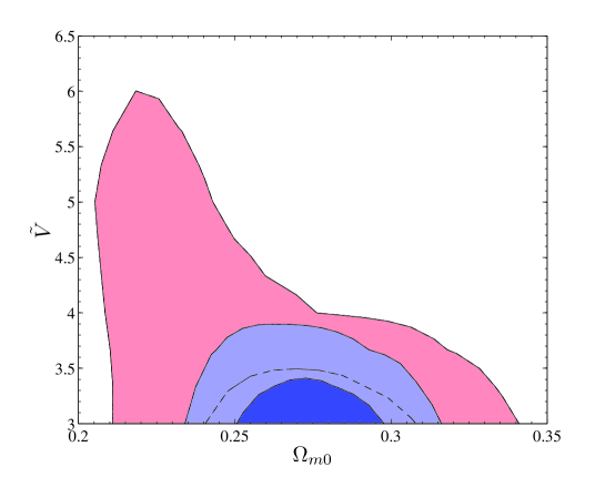
Figure 1: (Color Online) Two-dimensional likelihood contours in the ($\Omega_{m0},\tilde{V}$) plane for the $\epsilon=-1$ branch and fixed $\tilde{c}$ to its Randall-Sundrum value ($\tilde{c}=2\tilde{V}\rho_{r0}/\rho_{\ast}$) from the SnIa (red and pink) and SnIa+BAO (blue and light blue) data combinations. The light regions (pink and light blue respectively) correspond to 2$\sigma$ confidence level, while the darker regions (red and blue respectively) correspond to 1$\sigma$ confidence level. Note that in this specific plot the 1$\sigma$ bound of the SnIa (red) data combinations is inside the 2$\sigma$ bound of the SnIa+BAO (light blue) data combinations.

The $\mathcal{C}$-term in (3.6) corresponds to dark radiation, so it is proportional to $1/a^{4}$. This term, in particular $\Omega_{\mathcal{C}0}$, cannot be constrained efficiently by the low-redshift observations we are going to use in our analysis. However, since this dark radiation component was present at the time of Big Bang Nucleosynthesis (BBN) too, that is at redshift $z_{BBN}\sim 10^{9}$, we can use BBN arguments in order to constrain it. Specifically, the data impose an upper bound on the amount of total radiation (standard and exotic), which is expressed through the parameter $\Delta N_{\nu}$ of the effective neutrino species [34, 35, 36, 37]. Thus, in our case, this bound imposes a constraint on $\Omega_{\mathcal{C}0}$, namely

$$\Omega_{\mathcal{C}0}=0.135\Delta N_{\nu}\Omega_{r0}~{}.$$ (3.16)

The recently released Planck results impose a quite tight constraint on the effective number of neutrino species [33]: $N_{\rm eff}=3.30^{+0.54}_{-0.51}$ (95% C.L.) from the Planck+WP+highL+BAO data combination. Therefore, the 95% C.L. upper limit of $\Delta N_{\nu}$ is $\Delta N_{\nu}<0.776$. This leads to a very tight constraint on the dark radiation component of the scenario at hand, namely $\Omega_{\mathcal{C}0}<5\times 10^{-6}$ (95% C.L.). Thus, we can safely neglect this term in the remaining analysis and the remaining parameters to be fitted are $\tilde{c}$, $\tilde{V}$, $\rho_{\ast}$ and $\Omega_{m0}$.

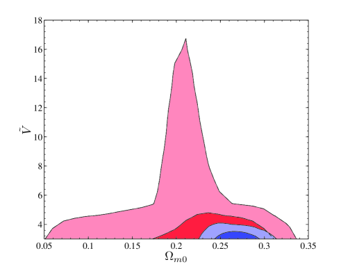
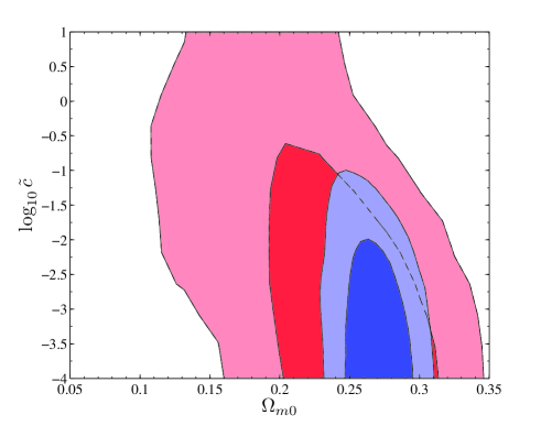
Figure 2: (Color Online) Two-dimensional likelihood contours in the ($\Omega_{m0},\tilde{V}$) and ($\Omega_{m0},\log_{10}\tilde{c}$) planes for the $\epsilon=-1$ branch from the SnIa (red and pink) and SnIa+BAO (blue and light blue) data combinations. The light regions (pink and light blue respectively) correspond to 2$\sigma$ confidence level, while the darker regions (red and blue respectively) correspond to 1$\sigma$ confidence level.

As a starting analysis, let us fit the case where $\tilde{c}$ is set to its value that corresponds to the standard braneworld cosmological scenario [28], namely $\tilde{c}=2\tilde{V}\rho_{r0}/\rho_{\ast}$ (which is exactly zero in the absence of radiation). Thus, in this case we have only three free parameters, namely $\tilde{V}$, $\rho_{\ast}$ and $\Omega_{m0}$. In Fig. 1 we provide the two-dimensional contour plots on ($\Omega_{m0},\tilde{V}$), using SnIa and SnIa+BAO data combinations. The details of the fitting procedure are presented in the Appendix. As we observe, when we use SnIa data only, the constraints on $\tilde{V}$ are relatively weak, namely $3<\tilde{V}<5.5$ at the $95\%$ confidence level. However, addition of the BAO data introduces an extra constraining power and the total constraint becomes tighter, namely $3<\tilde{V}<3.4$ ($95\%$ C.L.) from SnIa+BAO data. Finally, as we describe in the Appendix, the efficiency of the fitting is quantified by $\chi^{2}$, which for this case is $\chi^{2}\approx 570$.

Let us now proceed to the general case, that is considering $\tilde{c}$ as an additional free parameter. In the upper graph of Fig. 2 we present the contour plots of $\tilde{V}$ versus $\Omega_{m0}$, while in the lower graph of Fig. 2 we depict the contour plots of $\tilde{c}$ versus $\Omega_{m0}$. As we observe, the SnIa constraints on the parameter $\tilde{V}$ are much weaker than those of Fig. 1, due to the additional fitting variable. In particular, the 95% C.L. bound is $3<\tilde{V}<15.3$ (additionally note that the parameter space $\Omega_{m0}<0.2$ is now allowed by the SnIa data, exactly due to the presence of non-zero $\tilde{c}$). Concerning $\tilde{c}$ the SnIa data leads also to the relatively weak constraint $\log_{10}\tilde{c}<0.1$ (95% C.L.). However, for the combined SnIa with BAO data, the constraints become much tighter. At 95% confidence level they are $3<\tilde{V}<3.7$ and $\log_{10}\tilde{c}<-1.6$, while their best fit values are very close to 3 and 0 respectively. Finally, the corresponding $\chi^{2}$ is $\chi^{2}\approx 570$.

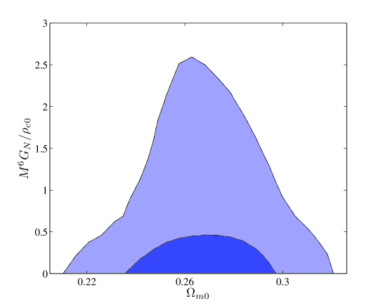
Figure 3: (Color Online) Two-dimensional likelihood contours of the dimensionless quantity $M^{6}G_{N}/\rho_{c0}$ versus $\Omega_{m0}$, where $\rho_{c0}$ is the current critical density, for the $\epsilon=-1$ branch from the SnIa+BAO data combinations. The lighter region corresponds to 2$\sigma$ confidence level, while the darker region corresponds to 1$\sigma$ confidence level.

Let us now refer to the constraints of the Cosmic Microwave Background (CMB) radiation on the scenario at hand. One can use such high-redshift probes, in particular the distance information of CMB, the shift parameter $R$ and the acoustic scale $\ell_{A}$, from WMAP9 or Planck data [33]. Their definitions are $R=\sqrt{\Omega_{m}H^{2}_{0}}\chi(z_{\ast})/c$ and $\ell_{A}=\pi\chi(z_{\ast})/\chi_{s}(z_{\ast})$, where $\chi(z_{\ast})$ and $\chi_{s}(z_{\ast})$ denote the comoving distance to the decoupling epoch $z_{\ast}$ and the comoving sound horizon at $z_{\ast}$, respectively. The current CMB data imply that at $z_{\ast}\sim 1100$ the Universe is dominated by matter, that is $H(z)^{2}\sim\rho_{m}(z)$. If in our model we neglect $\Omega_{k}$, $\Omega_{r}$ and $\Omega_{C}$ terms, and we insert the present value of the critical density $\rho_{c0}={3H_{0}^{2}}/{8\pi G_{N}}$, then (3.6) becomes $H^{2}=\rho_{m}(z)+\rho_{DE}(z)=H_{0}^{2}\Omega(z)$, where

$$\Omega(z) = \frac{1}{2}\left\{\left[\frac{{\Omega_{m0}}(1+z)^{3}}{\sqrt{\Omega_{\ast}\tilde{V}}}+\sqrt{\Omega_{\ast}\tilde{V}}\right]^{2}-9\frac{\Omega_{\ast}}{\tilde{V}}\right\},$$ (3.17)

with

$$\Omega_{\ast}\equiv\frac{\rho_{\ast}}{\rho_{c0}}.$$ (3.18)

Apparently, we deduce that if we want the term $\rho_{m}(z)^{2}$ to be significantly smaller than $\rho_{m}(z)$, we need

$$\frac{\left[\Omega_{m}(1+z)^{3}\right]^{2}}{\Omega_{\ast}\tilde{V}}\ll 2(\Omega_{m}(1+z)^{3})\ \ \Rightarrow\ \ \frac{\Omega_{m}(1+z)^{3}}{2\tilde{V}}\ll\Omega_{\ast}~{}.$$ (3.19)

Since $\tilde{V}\gtrsim 3$, it is implied that if we desire to satisfy the CMB data we need $\Omega_{\ast}\gg 0.05(1+z_{\ast})^{3}\sim 10^{7}$.

Proceeding forward, combining equations (2.17), (3.4) we obtain for the fundamental mass scale $M$ the relation

$$M^{6}=\frac{\tilde{V}\rho_{\ast}}{192\pi G_{N}}\,.$$ (3.20)

The likelihood contours of the dimensionless quantity $M^{6}G_{N}/\rho_{c0}$ versus $\Omega_{m0}$ is shown in Fig. 3. We can then straightforwardly estimate that at 1$\sigma$ confidence level $0<M<0.042\,\text{GeV}$. Moreover, to give an estimate for the value of the brane tension $V$, we use the relation $V=192\pi G_{N}M^{6}$, which leads to $0<V<2.22\times 10^{-44}\,\text{GeV}^{4}$ at 1$\sigma$ confidence level. That is $0<V<0.87\times 10^{3}\rho_{\Lambda 0}$, where $\rho_{\Lambda 0}$ is the current value of the energy density of the observed cosmological constant.

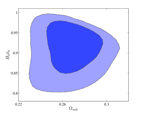
Figure 4: (Color Online) Two-dimensional likelihood contours of $H_{0}t_{0}$ versus $\Omega_{m0}$ for the $\epsilon=-1$ branch from the SnIa+BAO data combinations. The lighter region corresponds to 2$\sigma$ confidence level, while the darker region corresponds to 1$\sigma$ confidence level.

Finally, we close this subsection by examining the constraints on the model from the age of the universe. In general, the age of the universe is given by

$$t_{0}=\int_{0}^{\infty}\frac{dz}{(1+z)H(z)}\,,$$ (3.21)

where in the scenario at hand $H(z)$ is given by equation (3.13). Thus, taking into account the constraints on the model parameters elaborated above, we can construct the contour plots of $H_{0}t_{0}$ versus $\Omega_{m0}$, which is presented in Fig. 4. We can then straightforwardly estimate the age in Gyr, finding $12.23\ \text{Gyr}\leq t_{0}\leq 14.13\ \text{Gyr}$ at 1$\sigma$ confidence level (for the $\Lambda$CDM model with $\Omega_{m0}=0.28$ the corresponding age is 13.5 Gyr). We observe from equations (2.28) and (3.21) that larger values of the mass scale $M$ in the range found above correspond to larger values of the age of the universe. Thus, since larger ages are preferable, the most probable estimations for $M$ lie closer to the upper bound.

In summary, as we observe, the cosmological observations constrain $\tilde{V}$ and $\tilde{c}$ close to their Randall-Sundrum values, namely $\tilde{V}=3$ and $\tilde{c}\approx 0$ ($\tilde{c}=0$ in the case of radiation absence). However, note that the data allow for a departure from Randall-Sundrum scenario. In particular, although the present model has an additional parameter compared to Randall-Sundrum one, the corresponding $\chi^{2}$ is the same in two models, namely $\chi^{2}\approx 570$. This means that braneworld models with gravitating Nambu-Goto matching condition are in “equal” agreement with observations as the standard braneworld models.

Lastly, if we desire to compare the scenario at hand with the concordance paradigm of standard $\Lambda$CDM cosmology, we can be based on the Akaike Information Criterion (AIC) [38]

$$AIC=-2\ln{\mathcal{L}_{max}}+2k\,,$$ (3.22)

where $\,\ln{\mathcal{L}_{max}}=-\chi^{2}_{min}/2$ is the maximum likelihood achievable by the model (with $\chi^{2}_{min}/2$ the corresponding $\chi^{2}$ of the analysis) and $k$ the number of parameters of the model. Hence, we obtain the difference on the AIC between the standard $\Lambda$CDM cosmology and our gravitating Nambu-Goto matching conditions model as

$$\!\!\!\!\!\!\!\!\!\!\!\Delta AIC=AIC(\text{gravitating Nambu-Goto match. cond.})-AIC(\Lambda\text{CDM})$$

$$\ \ \ \ =\chi^{2}_{min}(\text{gravitating Nambu-Goto match. cond.})-\chi^{2}_{min}(\Lambda\text{CDM})+2\Delta{k},$$ (3.23)

where $\Delta{k}=k(\text{gravitating Nambu-Goto match. cond.})-k(\Lambda\text{CDM})$ is the difference of the number of parameters between the models. Thus, although in our model we obtain a $\chi^{2}_{min}$ similar to that of $\Lambda$CDM cosmology ($\chi^{2}_{min}(\Lambda\text{CDM})\approx 570$), the fact that we use two additional parameters gives $\Delta AIC\approx 4$. Thus, we deduce that $\Lambda$CDM cosmology is more favored comparing to the scenario at hand, since the two extra parameters do not improve the late-times fitting behavior.

3.2 Branch $\epsilon=+1$

In this case, the full Friedmann equation (2.28) is

$$H^{2}+\frac{k}{a^{2}}-\frac{\mathcal{C}}{a^{4}}=\Big{(}\frac{\rho_{\ast}}{24M^{3}}\Big{)}^{\!2}\,\Bigg{\{}\Bigg{[}\frac{\rho_{m}+\rho_{r}}{\rho_{\ast}}+\tilde{V}-\ \sqrt{\Big{(}\frac{\rho_{m}+\rho_{r}}{\rho_{\ast}}+\tilde{V}\Big{)}^{2}-2\tilde{V}\frac{\rho_{r}}{\rho_{\ast}}+\frac{\tilde{c}}{a^{4}}}\,\Bigg{]}^{2}-36\Bigg{\}}.$$ (3.24)

The branch $\epsilon=+1$ is completely new comparing to the standard braneworld models since the scale factor is bounded from above for any value of $\tilde{V}$. Therefore, contrary to the branch $\epsilon=-1$, here, there is no pure late-times linearization regime. However, expanding the expression (3.24), there is a term linear in $\rho_{m},\rho_{r}$, so Newton’s constant $G_{N}$ can also here be identified. More precisely it is $H^{2}+\frac{k}{a^{2}}-\frac{\mathcal{C}}{a^{4}}=\gamma(\rho_{m}+\frac{\rho_{r}}{2})+...$, where … do not contain terms linear in $\rho_{m},\rho_{r}$, and $\gamma=\frac{V}{144M^{6}}$. Therefore, associating $G_{N}$ with $\rho_{m}$ we have the identification

$$\gamma=\frac{V}{144M^{6}}\equiv\frac{8\pi G_{N}}{3}\,.\\$$ (3.25)

Going back to equation (3.24), we eliminate the parameter $M$ and we rewrite the expansion rate for $\epsilon=+1$ as

$$H^{2}+\frac{k}{a^{2}}-\frac{\mathcal{C}}{a^{4}}=\frac{4\pi G_{N}\rho_{\ast}}{3\tilde{V}}\Bigg{[} \!\!\!\tilde{V}\frac{2\rho_{m}+\rho_{r}}{\rho_{\ast}}+\Big{(}\frac{\rho_{m}+\rho_{r}}{\rho_{\ast}}\Big{)}^{2}+\tilde{V}^{2}-18+\frac{\tilde{c}}{2a^{4}}$$ (3.26)

$$\!\!-\Big{(}\frac{\rho_{m}\!+\!\rho_{r}}{\rho_{\ast}}\!+\!\tilde{V}\Big{)}\sqrt{\Big{(}\frac{\rho_{m}\!+\!\rho_{r}}{\rho_{\ast}}\!+\!\tilde{V}\Big{)}^{2}\!-\!2\tilde{V}\frac{\rho_{r}}{\rho_{\ast}}\!+\!\frac{\tilde{c}}{a^{4}}}\,\Bigg{]}\,.$$

This expression takes the standard form

$$H^{2}+\frac{k}{a^{2}}-\frac{\mathcal{C}}{a^{4}}=\frac{8\pi G_{N}}{3}(\rho_{m}+\rho_{r}+\rho_{DE}),$$ (3.27)

where

$$\rho_{DE}\!=\!\frac{\rho_{\ast}}{2\tilde{V}}\Bigg{[}\!\Big{(}\frac{\rho_{m}\!+\!\rho_{r}}{\rho_{\ast}}\Big{)}^{\!2}\!-\frac{\tilde{V}\rho_{r}}{\rho_{\ast}}+\tilde{V}^{2}-18+\frac{\tilde{c}}{2a^{4}}-\Big{(}\frac{\rho_{m}\!+\!\rho_{r}}{\rho_{\ast}}+\tilde{V}\Big{)}\sqrt{\Big{(}\!\frac{\rho_{m}\!+\!\rho_{r}}{\rho_{\ast}}\!+\!\tilde{V}\!\Big{)}^{2}\!\!-\!2\tilde{V}\frac{\rho_{r}}{\rho_{\ast}}\!+\!\frac{\tilde{c}}{a^{4}}}\,\Bigg{]}.$$ (3.28)

Defining the density parameters as in (3.8)-(3.12), we find equation (3.13), where $\rho_{DE}(z)$ is now given by

$$\!\!\!\!\!\!\rho_{DE}(z)=\frac{\rho_{\ast}}{2\tilde{V}}\Bigg{\{}\left(\frac{3H_{0}^{2}\Omega_{m0}}{8\pi G_{N}\rho_{\ast}}(1+z)^{3}+\frac{3H_{0}^{2}\Omega_{r0}}{8\pi G_{N}\rho_{\ast}}(1+z)^{4}\right)^{2}-\frac{3H_{0}^{2}\Omega_{r0}\tilde{V}}{8\pi G_{N}\rho_{\ast}}(1+z)^{4}+\tilde{V}^{2}-18$$

$$\quad\quad\quad\quad\quad\quad+\frac{\tilde{c}}{2}(1+z)^{4}-\left(\frac{3H_{0}^{2}\Omega_{m0}}{8\pi G_{N}\rho_{\ast}}(1+z)^{3}+\frac{3H_{0}^{2}\Omega_{r0}}{8\pi G_{N}\rho_{\ast}}(1+z)^{4}+\tilde{V}\right)\mathcal{A}(z)\Bigg{\}},$$ (3.29)

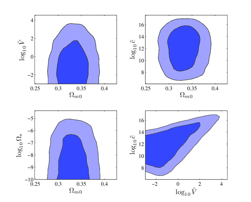
Figure 5: (Color Online) Two-dimensional likelihood contours in the ($\Omega_{m0},\tilde{V}$), ($\Omega_{m0},\log_{10}\tilde{c}$), ($\Omega_{m0},\Omega_{\ast}$) and ($\tilde{V},\log_{10}\tilde{c}$) planes, for the $\epsilon=+1$ branch, from the SnIa+BAO data combinations. The lighter regions correspond to 2$\sigma$ confidence level, while the darker region correspond to 1$\sigma$ confidence level.

with

$$\mathcal{A}(z)=\sqrt{\left(\frac{3H_{0}^{2}\Omega_{m0}}{8\pi G_{N}\rho_{\ast}}(1\!+\!z)^{3}+\frac{3H_{0}^{2}\Omega_{r0}}{8\pi G_{N}\rho_{\ast}}(1\!+\!z)^{4}+\tilde{V}\right)^{\!2}-\frac{3H_{0}^{2}\Omega_{r0}\tilde{V}}{4\pi G_{N}\rho_{\ast}}(1\!+\!z)^{4}+\tilde{c}(1\!+\!z)^{4}}\,.$$ (3.30)

In summary, Eq. (3.27) is the one we will fit, with $\mathcal{C}$, $\tilde{c}$, $\tilde{V}$, $\rho_{\ast}$ and $\Omega_{m0}$ as parameters (again for simplicity we fix $\Omega_{k0}$ to its (Planck+WP+highL+BAO) best fit values, namely $\Omega_{k0}=-0.0003$ [33]). Additionally, we include the direct $H_{0}$ probe from the Hubble Space Telescope (HST) observations of Cepheid variables with $H_{0}=73.8\pm 2.4$ ${\rm km\,s^{-1}\,Mpc^{-1}}$. Similarly to the previous subsection, we can safely neglect $\mathcal{C}$ since it is negligible according to BBN analysis. Finally, instead of $\rho_{\ast}$ it proves more convenient to introduce the dimensionless quantity (3.18), namely $\Omega_{\ast}\equiv\frac{\rho_{\ast}}{\rho_{c0}}$, where $\rho_{c0}$ is the present critical energy density of the Universe.

We use combined SnIa and BAO data to constrain $\tilde{c}$, $\tilde{V}$, $\Omega_{\ast}$ and $\Omega_{m0}$. In Fig. 5 we present the corresponding two-dimensional likelihood contours. Firstly, note that in this case $\tilde{V}$ is not theoretically restricted to values greater than 3 and in particular it is constrained in much smaller values, namely $\log_{10}\tilde{V}<2.0$ (95% C.L. upper limit). Additionally, note that since at late times $\rho_{DE}$ acquires negative values, the constraint on $\Omega_{\ast}$ is very close to zero, namely $\log_{10}\Omega_{\ast}<-5.5$ (95% C.L.). Due to the strong degeneracy between $\Omega_{\ast}$ and $\tilde{c}$, the constraints on $\tilde{c}$ are very different from those in the $\epsilon=-1$ branch case, namely $7.7<\log_{10}\tilde{c}<15.9$ (95% C.L.). However, note that the minimal $\chi^{2}$ for this case is $\chi^{2}\approx 688$, that is much higher than that for the $\epsilon=-1$ branch case, which means that the $\epsilon=+1$ branch case is not favored by observations. This can be additionally seen by calculating the corresponding age of the universe, which is much smaller than the $\Lambda$CDM value. However, although this branch is not favored by late-times observations, due to that $H^{2}\approx\text{const.}$ at early times, it could still play an important role in the inflationary regime.

4 Conclusions

In this work we constrained an alternative 5-dimensional braneworld cosmology using observational data. The difference with the standard braneworld cosmology refers to the adaptation of alternative matching conditions introduced in [16] which generalize the conventional matching conditions. The reasons for this consideration are possible theoretical deficiencies of the standard junction conditions, namely the need for consistency of the various codimension defects and the existence of a meaningful equation of motion at the probe limit. Instead of varying the brane-bulk action with respect to the bulk metric at the brane position and derive the standard matching conditions, we vary with respect to the brane embedding fields in a way that takes into account the gravitational back-reaction of the brane onto the bulk.

The proposed gravitating Nambu-Goto matching conditions may be close to the correct direction of finding realistic matching conditions since they always have the Nambu-Goto probe limit (independently of the gravity theory, the dimensionality of spacetime or codimensionality of the brane), and moreover, with these matching conditions, defects of any codimension seem to be consistent for any (second order) gravity theory. Compared to the conventional 5-dimensional braneworld cosmology, the new one possesses an extra integration constant, which if set to zero reduces the new cosmology to the conventional braneworld one.

In the present work we extended the codimension-1 cosmology of [27] by allowing both a matter and a radiation sector in order to extract observational constraints on the involved model parameters. In particular, we used data from supernovae type Ia (SNIa) and Baryon Acoustic Oscillations (BAO), along with arguments from Big Bang Nucleosynthesis (BBN) in order to construct the corresponding probability contour-plots for the parameters of the theory.

Concerning the first ($\epsilon=-1$) branch of cosmology, we found that the parameters $\tilde{V}$ and $\tilde{c}$ that quantify the deviation from the Randall-Sundrum scenario, are constrained very close to their RS values as expected. However, a departure from Randall-Sundrum scenario is still allowed, and moreover, the corresponding $\chi^{2}$ is the same for both models. This means that braneworld models with gravitating Nambu-Goto matching condition are in “equal” agreement with observations with standard braneworld cosmology. However, application of the AIC criterion shows that both standard braneworld cosmology, as well as the extended scenario of the present work, are less favored by the data if we compare them with the concordance $\Lambda$CDM cosmology since the two extra parameters do not improve the fitting behavior. Furthermore, the obtained age of the universe is $12.23\ \text{Gyr}\leq t_{0}\leq 14.13\ \text{Gyr}$, which is an additional observational advantage of the model. Finally, concerning the fundamental mass scale $M$, the current age estimations imply that the preferred values of $M$ lie well below the GeV scale.

Concerning the second ($\epsilon=+1$) cosmological branch, which is completely new and with no correspondence in Randall-Sundrum scenario, we extracted the corresponding likelihood contours. Although this case is still compatible with observations, the corresponding minimal $\chi^{2}$ is much higher than that for the $\epsilon=-1$ branch case, which means that this branch case is not favored by late-times observations. However, although this branch is not favored by late-times observations, due to that $H^{2}\approx\text{const.}$ at early times, it could still play an important role in the inflationary regime.

In summary, cosmology with gravitating Nambu-Goto matching conditions offers an extension to the standard Randall-Sundrum scenario. Apart from interesting solutions, we see that it is in agreement with observations since the data allow for a small deviation from Randall-Sundrum cosmology. Therefore, it should be worthy to further study the cosmological implications of the model, such as the inflationary behavior and the late-times asymptotic features, since especially a successful inflationary regime is something that cannot be obtained in the framework of $\Lambda$CDM cosmology.

Appendix A Observational data and constraints

In this Appendix we review the main procedures of observational fittings used in the present work, namely Type Ia Supernovae (SNIa) and Baryon Acoustic Oscillations (BAO).

a. Type Ia Supernovae constraints

We use the Union 2.1 compilation of SnIa data [39] in order to incorporate Supernovae type Ia constraints. This is a heterogeneous data set, which includes data from the Supernova Legacy Survey, the Essence survey and the Hubble-Space-Telescope observed distant supernovae.

The $\chi^{2}$ for this analysis is written as

$$\chi^{2}_{SN}=\frac{{\sum\limits_{i=1}^{N}{\left[{\mu_{\text{obs}}\left({z_{i}}\right)-\mu_{\rm th}\left({z_{i}}\right)}\right]}^{2}}}{{\sigma^{2}_{\mu,i}}},$$ (A.1)

where $N=580$ is the number of SNIa data points. In the above expression $\mu_{\rm obs}$ is the observed distance modulus, which is defined as the difference of the supernova apparent magnitude from its absolute one. Furthermore, $\sigma_{\mu,i}$ are the errors in the observed distance moduli, which are assumed to be uncorrelated and Gaussian, arising from a variety of sources. If we introduce the usual (dimensionless) luminosity distance $D_{L}(z;a_{i})$, calculated by

$$D_{L}\left(z;a_{i}\right)\equiv\left(1+z\right)\int^{z}_{0}dz^{\prime}\frac{H_{0}}{H\left(z^{\prime};a_{i}\right)},$$ (A.2)

with $H_{0}$ the present Hubble parameter, then the theoretical distance modulus $\mu_{\rm th}$ has a dependence on the model parameters $a_{i}$ as

$$\mu_{\rm th}\left(z\right)=42.38-5\log_{10}h+5\log_{10}\left[D_{L}\left(z;a_{i}\right)\right].$$ (A.3)

Finally, the marginalization over the present Hubble parameter is performed following [40], which eventually provides the $\chi^{2}$ likelihood contours for the model parameters that are involved.

b. Baryon Acoustic Oscillation constraints

In order to handle the baryon acoustic oscillation (BAO) observational constraints we use the definition [41]

$$A\equiv D_{V}(z=0.35)\frac{\sqrt{\Omega_{m}H^{2}_{0}}}{0.35c}=0.469\pm 0.017~{},$$ (A.4)

where $c$ is the light speed. In the above expression we have defined the “volume distance” $D_{V}\left(z\right)$ as

$$D_{V}\left(z\right)\equiv\left[\frac{\left(1+z\right)^{2}D_{A}^{2}(z)z}{H(z)}\right]^{1/3},$$ (A.5)

where

$$D_{A}\equiv r\left(z\right)/\left(1+z\right)$$ (A.6)

is the angular diameter distance. Finally, the BAO likelihood is written as

$$\chi^{2}_{BAO}=\frac{(A-0.469)^{2}}{0.017^{2}}~{}.$$ (A.7)

References

- [1] W. Israel, Singular hypersurfaces and thin shells in general relativity, Nuovo Cim. B 44S10, 1 (1966) [Erratum-ibid. B 48, 463 (1967)] [Nuovo Cim. B 44, 1 (1966)].
- [2] W. Israel, Line sources in general relativity, Phys. Rev. D 15, 935 (1977).
- [3] R. P. Geroch and J. H. Traschen, Strings and Other Distributional Sources in General Relativity, Phys. Rev. D 36, 1017 (1987) [Conf. Proc. C 861214, 138 (1986)].
- [4] D. Garfinkle, Metrics with distributional curvature, Class. Quant. Grav. 16, 4101 (1999), [arXiv:gr-qc/9906053].
- [5] A. Vilenkin, Gravitational Field of Vacuum Domain Walls and Strings, Phys. Rev. D 23, 852 (1981).
- [6] A. Vilenkin, Cosmic Strings and Domain Walls, Phys. Rept. 121, 263 (1985).
- [7] J. A. G. Vickers, Generalized Cosmic Strings, Class. Quant. Grav. 4, 1 (1987).
- [8] V. P. Frolov, W. Israel and W. G. Unruh, Gravitational Fields of Straight and Circular Cosmic Strings: Relation Between Gravitational Mass, Angular Deficit, and Internal Structure, Phys. Rev. D 39, 1084 (1989).
- [9] W. G. Unruh, G. Hayward, W. Israel and D. Mcmanus, Cosmic String Loops Are Straight, Phys. Rev. Lett. 62, 2897 (1989).
- [10] C. J. S. Clarke, J. A. Vickers and G. F. R. Ellis, The Large Scale Bending of Cosmic Strings, Class. Quant. Grav. 7, 1 (1990).
- [11] K. Nakamura, Comparison of the oscillatory behaviors of a gravitating Nambu-Goto string with a test string, Prog. Theor. Phys. 110, 201 (2003), [arXiv:gr-qc/0302057].
- [12] J. M. Cline, J. Descheneau, M. Giovannini and J. Vinet, Cosmology of codimension two brane worlds, JHEP 0306, 048 (2003), [arXiv:hep-th/0304147].
- [13] P. S. Apostolopoulos, N. Brouzakis, E. N. Saridakis and N. Tetradis, Mirage effects on the brane, Phys. Rev. D 72, 044013 (2005), [arXiv:hep-th/0502115].
- [14] P. Bostock, R. Gregory, I. Navarro and J. Santiago, Einstein gravity on the codimension 2-brane?, Phys. Rev. Lett. 92, 221601 (2004), [arXiv:hep-th/0311074].
- [15] C. Charmousis, G. Kofinas and A. Papazoglou, The Consistency of codimension-2 braneworlds and their cosmology, JCAP 1001, 022 (2010), [arXiv:0907.1640].
- [16] G. Kofinas and M. Irakleidou, Self-gravitating branes again, [arXiv:1309.0674].
- [17] D. Lovelock, The Einstein tensor and its generalizations, J. Math. Phys. 12, 498 (1971).
- [18] B. Zumino, Gravity Theories in More Than Four-Dimensions, Phys. Rept. 137, 109 (1986).
- [19] R. P. Geroch and P. S. Jang, Motion of a body in general relativity, J. Math. Phys. 16, 65 (1975).
- [20] J. Ehlers and R. P. Geroch, Equation of motion of small bodies in relativity, Annals Phys. 309, 232 (2004), [arXiv:gr-qc/0309074].
- [21] C. Germani and C. F. Sopuerta, String inspired brane world cosmology, Phys. Rev. Lett. 88, 231101 (2002), [arXiv:hep-th/0202060].
- [22] S. C. Davis, Generalized Israel junction conditions for a Gauss-Bonnet brane world, Phys. Rev. D 67, 024030 (2003), [arXiv:hep-th/0208205].
- [23] E. Gravanis and S. Willison, Israel conditions for the Gauss-Bonnet theory and the Friedmann equation on the brane universe, Phys. Lett. B 562, 118 (2003), [arXiv:hep-th/0209076].
- [24] R.C. Myers, Higher-derivative gravity, surface terms, and string theory, Phys. Rev. D 36 (1987) 392.
- [25] C. Charmousis and R. Zegers, Matching conditions for a brane of arbitrary codimension, JHEP 0508, 075 (2005), [arXiv:hep-th/0502170].
- [26] G. Kofinas and T. Tomaras, Gravitating defects of codimension-two, Class. Quant. Grav. 24, 5861 (2007), [arXiv:hep-th/0702010].
- [27] G. Kofinas and V. Zarikas, 5-dimensional braneworld with gravitating Nambu-Goto matching conditions, [arXiv:1312.4292].
- [28] P. Binetruy, C. Deffayet, U. Ellwanger and D. Langlois, Brane cosmological evolution in a bulk with cosmological constant, Phys. Lett. B 477, 285 (2000), [arXiv:hep-th/9910219].
- [29] C. Doolin and I. P. Neupane, Cosmology of a FLRW 3-brane, late-time cosmic acceleration, and the cosmic coincidence, Phys. Rev. Lett. 110, 141301 (2013), [arXiv:1211.3410].
- [30] A. Davidson and I. Gurwich, Dirac relaxation of the Israel junction conditions: Unified Randall-Sundrum brane theory, Phys. Rev. D 74, 044023 (2006), [arXiv:gr-qc/0606098].
- [31] L. Randall and R. Sundrum, A Large mass hierarchy from a small extra dimension, Phys. Rev. Lett. 83, 3370 (1999), [arXiv:hep-ph/9905221].
- [32] L. Randall and R. Sundrum, An Alternative to compactification, Phys. Rev. Lett. 83, 4690 (1999), [arXiv:hep-th/9906064].
- [33] P. A. R. Ade et al. [Planck Collaboration], Planck 2013 results. XVI. Cosmological parameters, [arXiv:1303.5076].
- [34] R. A. Malaney and G. J. Mathews, Probing the early universe: A Review of primordial nucleosynthesis beyond the standard Big Bang, Phys. Rept. 229, 145 (1993).
- [35] S. Dutta and E. N. Saridakis, Observational constraints on Horava-Lifshitz cosmology, JCAP 1001, 013 (2010), [arXiv:0911.1435].
- [36] S. Dutta and E. N. Saridakis, Overall observational constraints on the running parameter of Horava-Lifshitz gravity, JCAP 1005, 013 (2010), [arXiv:1002.3373].
- [37] K. Ichiki, M. Yahiro, T. Kajino, M. Orito and G. J. Mathews, Observational constraints on dark radiation in brane cosmology, Phys. Rev. D 66, 043521 (2002), [arXiv:astro-ph/0203272].
- [38] H. Akaike, A new look at the statistical model identification, Aut. Cont., IEEE Trans. on, 19, 6 (1974).
- [39] N. Suzuki, D. Rubin, C. Lidman, G. Aldering, R. Amanullah, K. Barbary, L. F. Barrientos and J. Botyanszki et al., The Hubble Space Telescope Cluster Supernova Survey: V. Improving the Dark Energy Constraints Above and Building an Early-Type-Hosted Supernova Sample, Astrophys. J. 746, 85 (2012), [arXiv:1105.3470].
- [40] R. Lazkoz, S. Nesseris and L. Perivolaropoulos, Comparison of Standard Ruler and Standard Candle constraints on Dark Energy Models, JCAP 0807, 012 (2008), [arXiv:0712.1232].
- [41] D. J. Eisenstein et al. (SDSS Collaboration), Astrophys. J. 633, 560 (2005).