IMPACTS OF ROTATION ON THREE-DIMENSIONAL HYDRODYNAMICS OF CORE-COLLAPSE SUPERNOVAE

Abstract

We perform a series of simplified numerical experiments to explore how rotation impacts the three-dimensional (3D) hydrodynamics of core-collapse supernovae. For the sake of our systematic study, we employ a light-bulb scheme to trigger explosions and a three-flavor neutrino leakage scheme to treat deleptonization effects and neutrino losses from proto-neutron star interior. Using a $15~{}M_{\odot}$ progenitor, we compute thirty models in 3D with a wide variety of initial angular momentum and light-bulb neutrino luminosity. We find that the rotation can help onset of neutrino-driven explosions for the models in which the initial angular momentum is matched to that obtained in recent stellar evolutionary calculations ($\sim 0.3$-$3$ rad s^-1 at the center). For the models with larger initial angular momentum, the shock surface deforms to be more oblate due to larger centrifugal force. This makes not only a gain region more concentrated around the equatorial plane, but also the mass in the gain region bigger. As a result, buoyant bubbles tend to be coherently formed and rise in the equatorial region, which pushes the revived shock ever larger radii until a global explosion is triggered. We find that these are the main reasons that the preferred direction of explosion in 3D rotating models is often perpendicular to the spin axis, which is in sharp contrast to the polar explosions around the axis that was obtained in previous 2D simulations.

1. INTRODUCTION

Multi-dimensionality in the inner working of core-collapse supernovae (CCSNe) has long been considered as one of the most important ingredients to understand the explosion mechanism. Shortly after the discovery of pulsars in the late 1960’s (Hewish et al., 1968), rotation and magnetic fields were first proposed to break spherical symmetry of the supernova engine (LeBlanc & Wilson, 1970; Bisnovatyi-Kogan et al., 1976; Müller & Hillebrandt, 1979). In the middle of 1980’s, the delayed neutrino-driven mechanism was proposed by Wilson (1985) and Bethe & Wilson (1985) who clearly recognized the importance of multi-dimensional (multi-D) effects (Wilson & Mayle, 1988). Ever since SN1987A, multi-D hydrodynamic simulations have been carried out extensively in a variety of contexts. They give us a confidence that multi-D hydrodynamic motions associated with PNS convection (e.g., Keil et al., 1996; Mezzacappa et al., 1998; Bruenn et al., 2004; Dessart et al., 2006), neutrino-driven convection (e.g., Herant et al., 1994; Burrows et al., 1995; Janka & Müller, 1996; Fryer, 2004; Murphy & Burrows, 2008), and the Standing-Accretion-Shock-Instability (SASI, e.g., Blondin et al., 2003; Ohnishi et al., 2006; Scheck et al., 2008; Foglizzo et al., 2006a; Iwakami et al., 2008, 2009; Kotake et al., 2009; Fernández & Thompson, 2009; Fernández et al., 2013, and see references therein) can help the onset of neutrino-driven explosions. In fact, a growing number of neutrino-driven models have been recently reported in the first-principle two-dimensional (2D) simulations (Buras et al. 2006a, b; Ott et al. 2008; Marek & Janka 2009; Bruenn et al. 2010, 2013; Suwa et al. 2010, 2013; Müller et al. 2012, 2013, however, Dolence et al. 2014).

This success, however, is bringing to light new questions. One of the outstanding problems is that the explosion energies obtained in these 2D models from first principles (though some of them were reported before their explosion energies saturated) are typically smaller by one order of magnitudes to explain the canonical supernova kinetic energy ($\sim 10^{51}$ erg, see Tables in Kotake (2013) and Papish et al. (2014) for a summary). Most researchers are now seeking for some possible physical ingredients to make these underpowered explosions more energetic (see Janka, 2012; Burrows, 2013; Kotake et al., 2012a, for recent reviews).

One of the major candidates is three-dimensional (3D) effects on the neutrino-driven mechanism. Employing a “light-bulb” scheme in 3D simulations, Nordhaus et al. (2010) were the first to point out that 3D leads to easier explosions than 2D. This was basically supported by some of the follow-up studies (Burrows et al., 2012; Dolence et al., 2013; Murphy et al., 2013), but not by 3D simulations with a similar setup (Hanke et al., 2012; Couch, 2013a) and by 3D simulations with spectral neutrino transport (Takiwaki et al., 2012; Hanke et al., 2013; Takiwaki et al., 2014). Another prime candidate is general relativity (GR), which has been agreed to help neutrino-driven explosions in both 2D (Müller et al., 2012, 2013) and 3D models (Kuroda et al. (2012), see also Ott et al. (2012); Kuroda et al. (2014)). The impacts of nuclear equations of state (EOS) have been investigated in 2D models (Marek & Janka, 2009; Marek et al., 2009; Suwa et al., 2013; Couch, 2013b), and these studies reached an agreement that softer EOS leads to easier explosions. The neutrino-driven mechanism could be assisted by the magnetohydrodynamic (MHD) mechanism that works most efficiently when the pre-collapse cores have rapid rotation and strong magnetic fields (e.g., Kotake et al. (2006) and Mösta et al. (2014) for collective references therein). It should be mentioned that even in the non-rotating case, the MHD mechanism assists the onset of explosion via the magnetic-field amplifications due to the SASI (Endeve et al., 2010, 2012; Obergaulinger & Janka, 2011). Other possibilities include nuclear burning behind the propagating shock (Bruenn et al., 2006; Nakamura et al., 2014; Yamamoto et al., 2013), additional heating reactions in the gain region (Sumiyoshi & Röpke, 2008; Arcones et al., 2008; Furusawa et al., 2013), hadron-quark phase transitions (e.g., Sagert et al., 2009; Fischer et al., 2012), or energy dissipation by the magnetorotational instability (Thompson et al., 2005; Obergaulinger et al., 2009; Masada et al., 2012; Sawai et al., 2013; Sawai & Yamada, 2014).

Joining in these efforts to look for some possible ingredients to foster explosions, we investigated the roles of rotation in this study. In 2D simulations of a $15M_{\odot}$ progenitor with detailed neutrino transport, Marek & Janka (2009) were the first to observe the onset of earlier explosions in models that include moderate rotation ($\Omega_{0}=0.5~{}{\rm rad}~{}{\rm s}^{-1}$ with $\Omega_{0}$ being the pre-collapse central angular velocity) than in models without rotation. By performing 2D simulations of an 11.2 $M_{\sun}$ star with more idealized spectral neutrino transport scheme (e.g., Liebendörfer et al., 2009), Suwa et al. (2010) showed that stronger explosion is obtained in models that include rapid rotation ($\Omega_{0}=2~{}{\rm rad}$ s^-1) than those without rotation. Suwa et al. (2010) also pointed out that rotation helps explosions, not only because the mass enclosed inside the gain radius becomes larger for rapidly rotating models, but also because north-south symmetric bipolar explosions that are generally associated with rapidly rotating models can expel much more material than that of one-sided unipolar explosions in the non-rotating models. These findings naturally open a simple question. Will these features so far obtained in 2D models also persist in 3D models?

In this study, we performed a series of simplified numerical experiments to explore how rotation impacts the 3D hydrodynamics of the CCSN core that produces an explosion by the neutrino mechanism. For the sake of our systematic study, we employed a light-bulb scheme to trigger explosions (e.g., Janka & Müller, 1996; Janka, 2001) and a three-species neutrino leakage scheme (e.g., Rosswog & Liebendörfer, 2003) to treat deleptonization effects and neutrino losses from the neutron star interior (above an optical depth of about unity). It is well-known from interferometric observations (see van Belle, 2012, for a review) that stars more massive than 1.5 $M_{\odot}$ are generally rapid rotators (Huang & Gies, 2006, 2008). However, due to numerical difficulties of multi-D stellar evolutionary calculations (see Maeder & Meynet (2012) for a review, and Meakin & Arnett (2007); Arnett & Meakin (2011) for recent developments), it is quite uncertain how such high surface velocities are entirely evolved during stellar evolution till the onset of core-collapse, in which multi-D hydrodynamics including mass-loss, rotational mixing, and magnetic braking is playing an active role in determining the angular momentum transport. In this study, we made pre-collapse models by parametrically adding the initial angular momentum to a widely used a 15 $M_{\odot}$ progenitor (Woosley & Weaver, 1995). We carried out 3D special-relativistic simulations starting from the onset of gravitational collapse, through bounce, trending towards explosions (typically up to about $\sim$1 s postbounce) and compare results of thirty 3D models, in which the input neutrino luminosity and the initial rotation rate are systematically varied. We found that a critical neutrino luminosity to obtain neutrino-driven explosions becomes generally smaller for models with larger initial angular momentum. Our 3D models show a much wider variety of the explosion geometry than in 2D. In the 3D rotating models, we found that the preferred direction of explosion is often perpendicular to the spin axis, which is in sharp contrast to polar explosions around the spin axis that was commonly obtained in previous 2D simulations.

We begin in Section 2 with a description of numerical setup and initial models. The main results are shown in Section 3. We summarize our results and discuss their implications in Section 4.

2. NUMERICAL SETUP

By utilizing the code developed by Kuroda & Umeda (2010) and Kuroda et al. (2012), we perform 3D, special-relativistic (SR) hydrodynamic simulations of the collapse, bounce, and post-bounce evolution of the core of massive stars. The basic evolution equations are written in a conservative form as,

$$\partial_{t}\rho_{\ast}+\partial_{i}(\rho_{\ast}v^{i}) = 0,$$ (1)

$$\partial_{t}S_{i}+\partial_{j}(S_{i}v^{j}+P\delta_{i}^{j}) = -\rho_{\ast}\partial_{i}\phi-Qu_{i},$$ (2)

$$\partial_{t}\tau+\partial_{i}(\tau v^{i}+Pv^{i}) = -\rho_{\ast}v^{i}\partial_{i}\phi-QW,$$ (3)

$$\partial_{t}(\rho_{\ast}Y_{e})+\partial_{i}(\rho_{\ast}Y_{e}v^{i}) = \rho_{\ast}\Gamma_{e},$$ (4)

where $\rho_{\ast}\equiv\rho W$, $S_{i}\equiv\rho hWu_{i}$, and $S_{0}\equiv\rho hW^{2}-P$ are auxiliary variables (corresponding to density, momentum, and energy), $\rho$ is the rest mass density, $W$ the Lorentz factor, $u_{\mu}$ the 4-velocity of fluid, $h\equiv 1+\varepsilon+P/\rho$ the specific enthalpy, $v^{i}=u^{i}/u^{0}$, $\tau=S_{0}-\rho_{\ast}$, $Y_{e}$ the electron fraction, $\varepsilon$ and $P$ the internal energy and pressure, $\delta_{i}^{j}$ the Kronecker delta, respectively. We employ the EOS based on the relativistic mean-field theory of Shen et al. (1998). As pointed out by Suwa et al. (2013) and Couch (2013b), the use of Lattimer-Swesty EOS with an incompressibility modulus of $K=220$ MeV (LS220), which is another representative EOS employed in modern CCSN simulations, would lead to easier explosion because LS220 EOS is softer than Shen EOS. Detailed analysis to clarify the impacts of EOS in rotating core-collapse models remains to be studied in the future work.

In the right-hand-side of above equations, $\phi$ represents gravitational potential, $Q$ and $\Gamma_{e}$ denote exchange of energy-momentum and lepton number between neutrino and matter. To solve the Poisson equation of self-gravity ($\nabla^{2}\phi=4\pi S_{0}$), we employ a “BiConjugate Gradient Stabilized (BiCGSTAB)” method with an appropriate boundary condition (see Kuroda et al. (2012) for further details).

The neutrino-matter interaction term $Q$ is divided into cooling and heating terms ($Q=Q^{C}+Q^{H}$). Following a methodology of a multi-flavor neutrino leakage scheme (e.g., Rosswog & Liebendörfer, 2003), the cooling term can be estimated as,

$$Q^{C} =Q_{e^{-}}^{f}+Q_{e^{-}}^{h}+Q_{e^{+}}^{f}+Q_{e^{+}}^{h}$$ (5)

$$+ \sum_{\nu\in(\nu_{e},\bar{\nu}_{e},\nu_{x})}2(Q_{e^{-}e^{+}\rightarrow\nu\bar{\nu}}+Q_{\gamma\rightarrow\nu\bar{\nu}}+Q_{NN\rightarrow NN\nu\bar{\nu}}),$$

where $Q_{e^{-/+}}^{f}$ and $Q_{e^{-/+}}^{h}$ represents the cooling rate by electron/positron capture on free nucleons and on heavy nuclei, $Q_{e^{-}e^{+}\rightarrow\nu\bar{\nu}}$, $Q_{\gamma\rightarrow\nu\bar{\nu}}$, and $Q_{NN\rightarrow NN\nu\bar{\nu}}$ denote contributions from pair neutrino annihilation, plasmon decay, and nucleon-nucleon bremsstrahlung, respectively (see Kuroda et al. (2012) for more detail). Following Janka (2001) and Murphy & Burrows (2008), we employ a simple light-bulb scheme to estimate $Q^{H}$ as,

$$Q^{H}=1.544\times 10^{20}\left(\frac{L_{\nu_{\rm e}}}{10^{52}\,{\rm erg\,s^{-1}}}\right)\left(\frac{T_{\nu_{e}}}{4{\rm MeV}}\right)^{2}$$

$$\times\left(\frac{r}{100{\rm km}}\right)^{-2}(Y_{\rm n}+Y_{\rm p})e^{-\tau}{\rm[erg/g\,s]},$$ (6)

where $L_{\nu_{\rm e}}$ is the electron-neutrino luminosity that is assumed to be equal to the anti-electron neutrino luminosity ($L_{\bar{\nu}_{\rm e}}=L_{\nu_{\rm e}}$), $T_{\nu_{\rm e}}$ is the electron neutrino temperature assumed to be kept constant as $4$ MeV, $r$ is the distance from the center, $Y_{n}$ and $Y_{p}$ are the neutron and proton fractions, and $\tau$ is the electron neutrino optical depth that we estimate from Equation (7) in Hanke et al. (2012).

As already mentioned, we add pre-collapse rotation to the non-rotating 15$M_{\odot}$ model (Woosley & Weaver, 1995, model “s15s7b2”) to study its effect in a controlled fashion. We assume a shell-type rotation profile as

$$\Omega(r)=\Omega_{0}\frac{R_{0}^{2}}{r^{2}+R_{0}^{2}},$$ (7)

where $\Omega(r)$ is the angular velocity at the radius of $r$, $R_{0}$ set here to be $2\times 10^{8}$ cm is reconciled with results from stellar evolution calculations suggesting uniform rotation in the pre-collapse core. The initial angular velocity at the origin, $\Omega_{0}$, is treated as a free parameter and we vary it as $\Omega_{0}=0,\ 0.1\,\pi,$ and $0.5\,\pi$ rad s^-1. Note that these angular velocities are in good agreement with the outcomes of most recent stellar evolution models that were evolved with the inclusion of magnetic fields ($\Omega_{0}\sim 0.2$-$0.3$ rad s^-1 of models m15b4 and m20b4 in Heger et al., 2005) or without the magnetic braking ($\Omega_{0}\sim 3$-$4$ rad s^-1 of models E15 and E20 in Heger et al., 2000).

The 3D computational domain consists of a cube of $10000^{3}~{}{\rm km}^{3}$ volume in the Cartesian coordinates. Nested boxes with nine refinement levels are embedded in the computation domain. We use a fiducial resolution at the maximum refinement level (the minimum grid scale) of $\Delta x_{\rm min}=600$ m in each direction. Each block has $64^{3}$ cubic cells. Roughly speaking, such structure corresponds to an angular resolution of $\sim 2$ deg through the entire computational domain. To study the resolution dependence of our results, we perform high resolution runs for some selected models, in which each nested block has $128^{3}$ cubic cells (i.e. $\Delta x_{\rm min}=300$ m at the centre). Note that the numerical resolutions in the central region are almost similar or slightly better comparing to recent 3D Newtonian simulations with a similar treatment of the neutrino effects ($\Delta x_{\rm min}=700$ m of Couch, 2013a), as well as GR simulations ($\Delta x_{\rm min}=370$ m of Ott et al., 2012), although Ott et al. (2012) adopted the leakage scheme for both heating and cooling.

Table 1Model Summary

	$\Omega_{0}=0.0$ (rad s-1)				$\Omega_{0}=0.1\,\pi$ (rad s-1)				$\Omega_{0}=0.5\,\pi$ (rad s-1)
${L_{\nu,52}}^{a}$	${t_{\rm exp}}^{b}$	$\dot{M}$c	shaped		$t_{\rm exp}$	$\dot{M}$	shape		$t_{\rm exp}$	$\dot{M}$	shape
($10^{52}\,{\rm erg\,s}^{-1}$)	(ms)	($~{}M_{\odot}\,{\rm s}^{-1}$)			(ms)	($~{}M_{\odot}\,{\rm s}^{-1}$)			(ms)	($~{}M_{\odot}\,{\rm s}^{-1}$)
1.5					—	—	—		135	0.426	oblate
1.7					541	0.263	oblate		128	0.469	oblate
1.9					500	0.264	oblate		117	0.579	oblate
2.1					355	0.293	oblate		108	0.679	oblate
2.3	—	—	—		336	0.300	oblate		90	0.907	oblate
					563∗,e	0.264∗	oblate∗
2.5	—	—	—		348	0.295	oblate		93	0.864	oblate
					203∗	0.356∗	spher.∗
2.7	—	—	—		229	0.345	oblate		70	1.09	oblate
					128∗	0.469∗	spher.∗
2.9	207	0.355	spher.		57	1.20	spher.
					75∗	1.05∗	spher.∗
3.1	168	0.369	spher.
3.3	140	0.404	spher.
3.5	47	1.31	spher.
a Electron-neutrino luminosity.
b Postbounce time of onset of explosion. Models that have a blank entry in the table are
not simulated and the “—” symbol indicates that the model does not explode.
during the simulated period of evolution.
c Mass accretion rate at onset of explosion.
d Morphological classification of shock shape at $t=t_{\rm exp}$. See the text for definition.
e The values with an asterisk symbol “xxx∗” indicates that the values are obtained in the higher
resolution model ($\Delta x_{\rm min}=300$m) compared to our fiducial resolution of $\Delta x_{\rm min}=600$m.

3. RESULTS

3.1. Overview of Simulation Results

Following the previous investigations (e.g., Murphy & Burrows, 2008; Nordhaus et al., 2010; Hanke et al., 2012; Couch, 2013a), we first take the approach of Burrows & Goshy (1993), using critical neutrino luminosity versus accretion rate to overview the impacts of rotation. Hereafter the neutrino luminosity is referred to as $L_{\nu,52}$ in unit of $10^{52}$ erg s^-1, and the initial angular velocity $\Omega_{0}$ in Equation (7) is given in unit of rad s^-1 unless otherwise noted.

For three cases of rotation ($\Omega_{0}=0.0$, $0.1\,\pi$, and $0.5\,\pi$), Table 1 summarizes the time of explosion, $t_{\rm exp}$, the mass accretion rate, $\dot{M}$, and the shape of shock front, as a function of $L_{\nu,52}$. Here as in Nordhaus et al. (2010) and Hanke et al. (2012), we define $t_{\rm exp}$ as the time when the shock reaches an average radius of 400 km (and does not returns later on). $\dot{M}$ is estimated at $t=t_{\rm exp}$ and $r=500$ km. The shock configuration is defined by the ratio of shock radius around the equatorial plane to that in the polar directions at $t_{\rm exp}$. The shock morphology is discussed in more detail in the last of §3.1.

Given an input luminosity, for example $L_{\nu,52}=2.5$, the non-rotating model ($\Omega_{0}=0.0$) does not explode till 1 second after bounce (so the model is labeled as “—”). On the other hand, the corresponding model with moderate rotation ($\Omega_{0}=0.1\,\pi$) explodes at $t_{\rm exp}=348$ ms postbounce and the rapidly rotating model ($\Omega_{0}=0.5\,\pi$) explodes much faster (at $t_{\rm exp}=93$ ms). This is a common trend for models with the input luminosity below $L_{\nu,52}=2.9$. The critical value of the neutrino luminosity and accretion rate of the non-rotating model is $L_{\nu,52}=2.9$ and $\dot{M}\sim 0.36~{}M_{\odot}~{}{\rm s}^{-1}$ (Table 1). Note that these values for the critical neutrino luminosity and the critical mass accretion rate in the non-rotating model are roughly in agreement with those obtained in previous 3D simulations with the light-bulb scheme (e.g., $L_{\nu,52}=2.5$ in Hanke et al. (2012) and $L_{\nu,52}=2.1$ in Couch (2013a) for $\dot{M}\sim 0.3~{}M_{\odot}~{}{\rm s}^{-1}$).

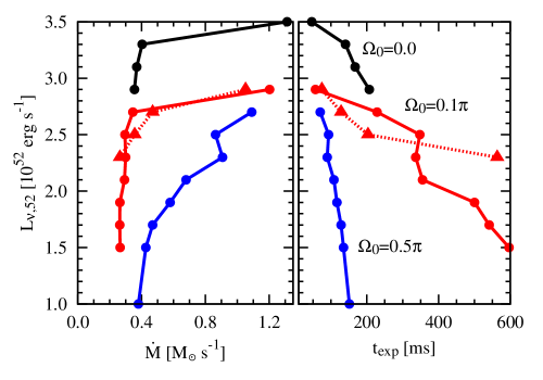
Figure 1.— Critical curves for the neutrino luminosity $L_{\nu,52}$ versus mass accretion rate ($\dot{M}$, left plot) and versus explosion time ($t_{\rm exp}$, right plot) for simulations with $\Omega_{0}=0.0$ (black), $0.1\,\pi$ (red), and $0.5\,\pi$ rad (blue). The time of explosion is defined at the moment when the average shock radius reaches 400 km, and accretion rate is measured at the distance of 500 km from the center at the time of $t_{\rm exp}$. Two cases of spatial resolution are shown in each panel, the fiducial resolution ($\Delta x_{\rm min}=600$m) by solid lines with filled circles and the high resolution ($\Delta x_{\rm min}=300$m) by dashed lines with filled triangles.

The left panel of Figure 1 shows the $L_{\nu,52}$-$\dot{M}$ curves for all the computed models with different initial rotation rates of $\Omega_{0}=0.5\,\pi$ (blue line), $0.1\,\pi$ (red line), and $0.0$ (black line). Compared to the non-rotating models (black line), the critical luminosities are shown to be smaller by $\sim 50\%$ for the mildly rotating models (red line) and by $\sim 70\%$ for the rapidly rotating models (blue line). These results demonstrate that rotation could result in easier explosions compared to the non-rotating models. Very recently, Iwakami et al. (2014) obtained qualitatively the same results with an ideal initial setup.

Not surprisingly, a high driving luminosity is necessary to overcome a high mass accretion rate regardless of rotation (left panel), which results in earlier onset of explosion (right panel). These features are qualitatively in accord with those obtained in previous parameterized 3D models without rotation (e.g., Burrows et al., 2012; Dolence et al., 2013; Hanke et al., 2012). Here it should be noted that the initial angular momentum of our moderately-rotating models ($\Omega_{0}=0.1\,\pi$) is not as rapid as previously assumed (Marek & Janka, 2009; Suwa et al., 2010), but as slow as that predicted by the most recent stellar evolution calculation (Heger et al., 2005). As we discuss more in detail in the following, even such a slow rotation can significantly effect the shock revival and evolution in the postbounce phase.

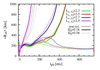
Figure 2.— Time evolution of the average shock radius as a function of the postbounce time $t_{\rm pb}$ for 3D models with rapid rotation ($\Omega_{0}=0.5\,\pi$, dotted lines), moderate rotation ($\Omega_{0}=0.1\,\pi$, solid lines), and no rotation (dashed lines). Different electron-neutrino luminosity (in unit of $10^{52}~{}{\rm erg}~{}{\rm s}^{-1}$, $L_{\nu,52}$) is plotted in different colors.

Figure 2 shows time evolution of average shock radius $\langle R_{\rm sh}\rangle$ for some selected luminosity models ($L_{\nu,52}$ between 2.3 and 2.9 presented in different colors) with the different rotation parameters ($\Omega_{0}=0$ in dashed lines, $\Omega_{0}=0.1\,\pi$ in solid lines, and $\Omega_{0}=0.5\,\pi$ in thin dotted lines). Without rotation (dashed lines), one can see that the bounce shock all stalls at the radius of $r\sim 200$ km as in previous 3D models with similar microphysical setup (Hanke et al., 2012; Dolence et al., 2013). As is expected, the maximum shock extent afterwards is bigger for models with higher input luminosity (i.e., biggest for the dashed pink line ($L_{\nu,52}=2.9$), followed in order by the dashed blue ($L_{\nu,52}=2.7$), dashed red ($L_{\nu,52}=2.5$), and dashed green line ($L_{\nu,52}=2.3$)). Except for the highest luminosity model (with $L_{\nu,52}=2.9$, dashed pink line), the late-time shock trajectory of the non-rotating models similarly shows a continuous recession and the stalled shock never revives during the simulation time.

When these models have moderate rotation initially ($\Omega_{0}=0.1\,\pi$, solid lines), the shock trajectories show a clear deviation from those without rotation. This occurs typically after $\sim 200$ ms postbounce (see the bifurcation points between the solid and dashed lines for models with $L_{\nu,52}=$ 2.3 (green), 2.5 (red), and 2.7 (blue). This clearly demonstrates that even the moderate pre-collapse rotation could effect the shock evolution. When the initial rotational speed is very fast ($\Omega_{0}=0.5\,\pi$, thin dotted lines), the shock revival occurs very quickly after bounce even for the model with the lowest luminosity. We will address the reasons of such interesting behaviors from the next secsion. Before going into detail, we briefly summarize how rotation impacts the 3D blast morphology in the following.

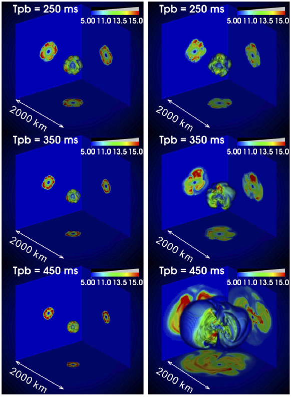
Figure 3.— Snapshots of 3D entropy distribution in the fiducial resolution. The non-rotating ($\Omega_{0}=0.0$, left panels) and moderately rotating ($\Omega_{0}=0.1\,\pi$, right panels) models are computed with the same input luminosity of $L_{\nu,52}=2.5$. Top, middle, and bottom panel corresponds to the timeslice of $t_{\rm pb}=250$ ms, 350 ms, and 450 ms postbounce, respectively. The vertical axis is aligned with the rotational axis. Note that spatial scale is different between the left ($600^{3}$ km³) and right ($2000^{3}$ km³) panels.

Figure 3 shows several snapshots of 3D entropy distribution of the $L_{\nu,52}=2.5$ model without rotation ($\Omega_{0}=0.0$, left panels) and with moderate rotation ($0.1\,\pi$, right) at $t_{\rm pb}=250$ ms (top), 350 ms (middle), and 450 ms (bottom), respectively. After the bounce shock stalls (top left panel), the shape of the shock keeps to be roundish all the way for the non-rotating model (from top left to bottom left), which does not trend towards explosion during the simulation time (see also red dashed line in Figure 2). If the input luminosity is taken to be higher for the non-rotating model, we observe a strong correlation, as previously identified, between large-scale structures; high entropy plumes (red regions in the sidewall panels) are associated with outflows whereas low-entropy regions (blueish regions) are associated with inflows, a natural outcome of buoyancy-driven convection (Murphy et al., 2013; Burrows et al., 2012; Dolence et al., 2013; Hanke et al., 2012). These postshock structures are clearly different from the same luminosity model but when moderate rotation is initially imposed ($\Omega_{0}=0.1\,\pi$, right panels in Figure 3). An important difference between the non-rotating and rotating model is the existence of more big-scale structure in the flow of the rotating model, which can be seen as an oblate structure in the postshock regions (e.g., green regions in the middle right panel; taken at $t_{\rm pb}=350$ ms when the shock reaches to the average radius of 400 km). The natural outcome is an oblate explosion as shown in the bottom right panel.

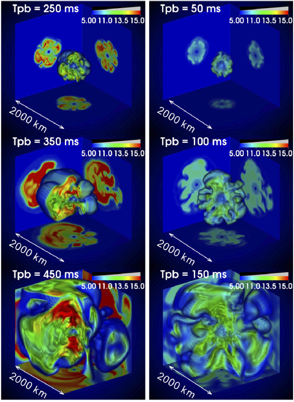
Figure 4.— Same as Figure 3 but for different input luminosity of $L_{\nu,52}=2.7$ (left panels) and $2.9$ (right panels) with the same initial rotation rate (moderate rotation; $\Omega_{0}=0.1\,\pi$).

The morphology of the revived shock is diverse from models to models. A snapshot presented in the top left panel of Figure 4 (model $L_{\nu,52}=2.7$ with $\Omega_{0}=0.1\,\pi$) shows a clear rotational flattening in the postshock region, which is a typical feature caused by $l=2$ mode in the rotating core collapse and bounce. The revived shock of this model (red regions in the middle left panel) is also deformed to be oblate. The oblately deformed shock moves out triaxially afterwards, leading to a strong shock expansion to the equatorial direction rather in an one-sided way (bottom left panel). For the same initial rotation rate, the oblateness is shown to appear more weakly in the model with higher input luminosity ($L_{\nu,52}=2.9$, right panels in Figure 4). This is because in models with higher luminosity the violent fluid motions as well as vigorous convective overturns work to smear out the effects of rotation (e.g., Kotake et al., 2011). This trend is clearly seen in Table 1, where the degree of shock deformation is evaluated as the ratio of shock radius averaged over $60^{\circ}\leq\theta\leq 120^{\circ}$ to that around the rotation axis ($\theta<60^{\circ}$, $120^{\circ}<\theta$). We define shocks with this ratio between $0.45$ and $0.55$ as ${\it spherical}$, and shocks with this ratio superior/inferior to this range is referred to as ${\it oblate/prolate}$.

To focus on the shock deformation, constant entropy contours are shown in Figure 5. By comparing with Figures 3 and 4 with Figure 5, one could more clearly see that the blast morphology is close to be oblate (top panels and middle left panel in Figure 5), one-sided (middle right panel), and multi-polar (roundish, bottom panels), respectively. As mentioned above, the high neutrino luminosity (e.g., bottom panels in Figure 5) tends to wash away the impacts of rotation, so that we mainly focus on models with smaller luminosity ($L_{\nu,52}\leq 2.9$) in the following.

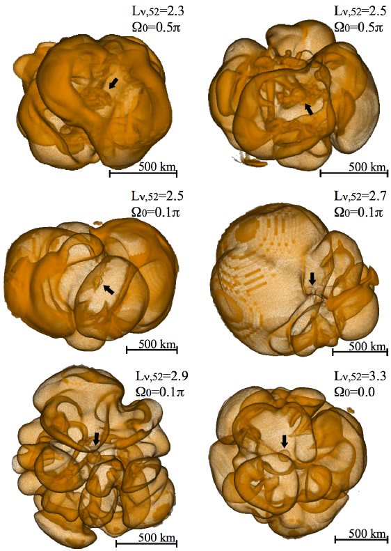
Figure 5.— Various structures of shocked gas in our models. Shown are the isentropic surface of $8\,k_{\rm B}$ per baryon shortly after the shock revival. Neutrino luminosity and angular velocity parameters are labeled in each panel. A obscure sphere pointed by an arrow in each panel corresponds to the position of PNSs (defined by a fiducial density of $10^{11}~{}{\rm g}{\rm cm}^{-3}$ as in Müller et al., 2012; Suwa et al., 2013).

Before going to the next section, we shall note that the above results are qualitatively little affected by the employed numerical resolution. Then what about the quantitative dependence? Due to the computational expense, we can currently afford to run four high-resolution models in 3D (that we chose to have the canonical initial rotation rate, $\Omega_{0}=0.1$). As in Hanke et al. (2012), our high-resolution models lead to more delayed explosions compared to the low-resolution counterpart when the input luminosity is as low as that in Hanke et al. (2012) (see our lowest luminosity model with $L_{\nu,52}=2.3$ in the right panel of Figure 1 (dashed red curve) which shows the (diagnostic-)explosion time of $t_{\rm exp}\sim 600$ ms). On the other hand, our models, switching to high-resolution, show earlier explosions ($t_{\rm exp}\lesssim 200$ ms postbounce) when the input luminosity is relatively higher ($L_{\nu,52}\gtrsim 2.5$). We would speculate that high numerical resolution could capture more efficiently the growth of such highly convection-dominated explosions in the case of such high luminosity. Further numerical experiments are apparently needed (at least to get a convergence in 3D), which unfortunately demands us a formidable computational cost at present.

3.2. Detailed Comparison between Non-rotating and Rotating Models

In this section, we move on to look in more detail into the reason why rotation could result in easier explosion. As will be shown, the key is the increase of the total gain mass for models with rotation, which is a natural outcome of the rotational flattening of the postshock region. In the following, we use the $L_{\nu,52}=2.5$ models as a reference, for which the shock revival is not obtained in the non-rotating model but is observed when moderate rotation ($\Omega_{0}=0.1~{}\pi$) is taken into account (see red lines in Figure 2).

3.2.1 Gain Mass

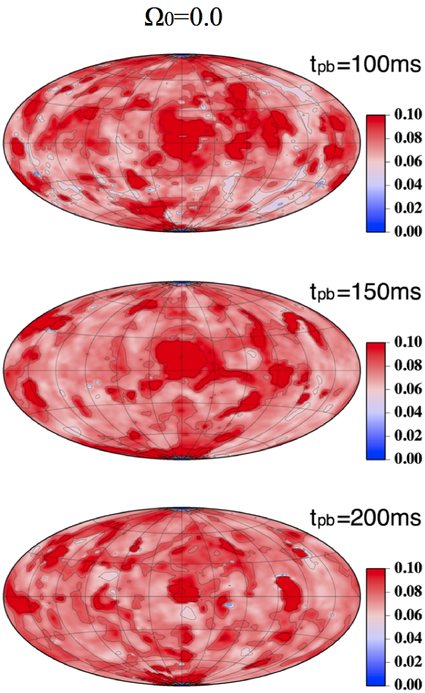
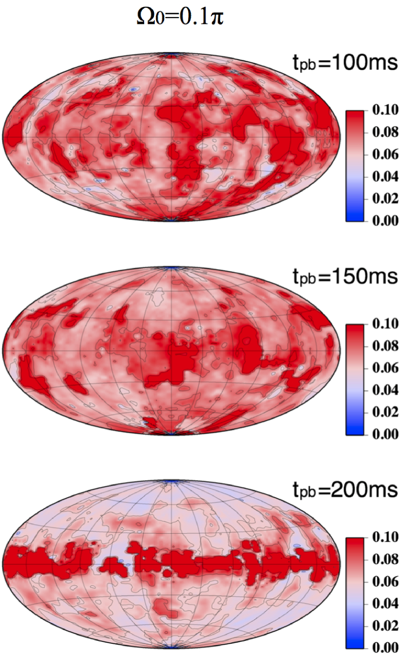
Figure 6.— Mollweide maps showing the mass distributions in the gain region for the $L_{\nu,52}=2.5$ model with $\Omega_{0}=0.0$ (left) and $0.1\,\pi$ (right) at $t_{\rm pb}=100$ ms, 150 ms, and 200 ms postbounce (from top to bottom), respectively. The color scale shows the mass fraction of the gain region in each solid angle (normalized by the total mass in the gain region).

It is well known that the enclosed mass in the gain region (the so-called gain mass), if bigger (smaller), does good (harm) to the revival of the stalled bounce shock. As a guide to see how rotation affects the gain mass and its spatial distributions, we plot in Figure 6 the Mollweide maps of the gain-mass distributions for the $L_{\nu,52}=2.5$ model without (left panels) and with rotation (right panels), respectively. Throughout our simulation time, the spatial distribution of the gain mass stochastically changes (as anticipated) for the non-rotating model (left panels, see red regions), whereas a clear excess is seen for the rotating model in the vicinity of the equatorial plane (seen like a belt, bottom right panel). The excess is clearly seen typically after $\sim$ 200 ms postbounce, but a gradual concentration to the equatorial belt (red regions in the equatorial region) can be also seen at 150 ms postbounce (middle right panel).

Figure 7.— Evolution of the mass in the gain region for the $L_{\nu,52}=2.5$ model with $\Omega_{0}=0.0$ (dashed thin line) and $\Omega_{0}=0.1\,\pi$ (solid thick line). Top and bottom panel shows the total mass in the gain region and the gain-mass ratio, respectively, the latter of which is defined to be the mass fraction of the gain region in the range of $60^{\circ}\leq\theta\leq 120^{\circ}$ to the total mass (see the text for more detail).

From Figure 7, one can also see that the gain mass of the rotating model (solid line in the top panel), which is almost identical to that of the non-rotating model (dashed line) until $t_{\rm pb}\lesssim 140-160$ ms, gradually increases later on. Due to the centrifugal forces, the postshock regions deform to be oblate (e.g., middle left panel of Figure 5). This acts to enlarge the gain region in the equatorial region. Note in the bottom panel of Figure 7 that the gain-mass fraction for the non-rotating model (dashed line) is close to 0.5 in the equatorial belt (over $60^{\circ}\leq\theta\leq 120^{\circ}$ with $\theta$ representing the polar angles) as it should be because the gain mass is randomly distributed (see again left panels in Figure 6). For the rotating model, the ratio exceeds 0.5, which clear shows the excess of the gain mass in the equatorial region.

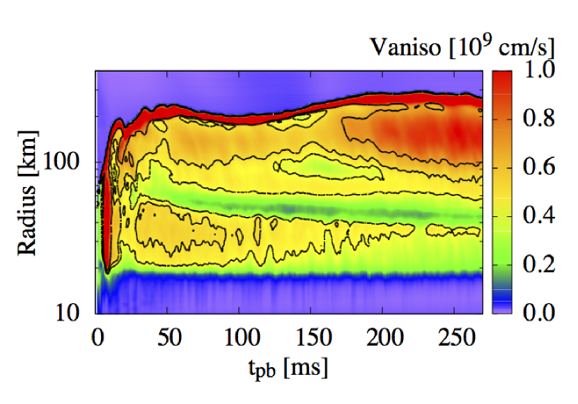
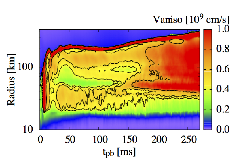
Figure 8.— Radial distribution of anisotropic velocity in unit of $10^{9}$ cm s^-1. Two cases of $L_{\nu,52}=2.5$ without rotation (left) and with $\Omega_{0}=0.1~{}\pi$ (right) are shown as functions of the postbounce time, respectively.

Figure 8 shows the time evolution of anisotropic velocity (Takiwaki et al., 2012) which we slightly change the definition to fit to the analysis of rotating models as

$$v_{\rm aniso}=\sqrt{\langle\rho\left((v_{r}-\langle v_{r}\rangle)^{2}+v_{\theta}^{2}+(v_{\phi}-\langle v_{\phi}\rangle)^{2}\right)\rangle/\langle\rho\rangle},$$ (8)

in which $\langle\rangle$ denotes an average value over angles perpendicular to the radial direction. As seen from the right panel of Figure 8, matter with high anisotropic motions (red regions) starts to move outward at $t_{\rm pb}\sim 140$-$160$ ms for the rotating model. This is closely correlated with the time when the gain mass in the equatorial region starts to gradually increase (Figure 7). The growth of such highly convective regions also works to enhance the efficiency of neutrino heating because it makes longer the residence time of accreting matter in the gain region. A brief summarize in this subsection is that the rotational flattening of the postshock region and the resulting increase of the total gain mass is primarily important to understand the reason of easier explosions of our 3D rotating models.

3.2.2 Mode Analysis: SASI versus Neutrino-driven Convection

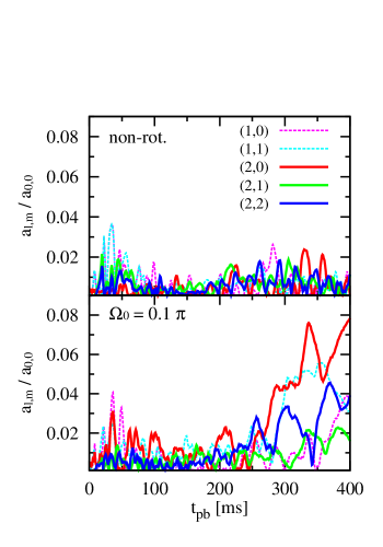
Figure 9.— Time evolution of the normalized spherical harmonic mode amplitudes ($Y_{\ell,m}$) for each set of (${\ell,m}$) for the $L_{\nu,52}=2.5$ model without rotation (top) and with moderate rotation ($\Omega_{0}=0.1\,\pi$, bottom).

Now we move on to perform a mode analysis of the shock regarding the reference models in the last secsion (Figure 9). Comparing with the top to the bottom panel, it can be seen that the sloshing mode of $(\ell,m)=(2,0)$ (red line) for the rotating model is clearly bigger than that of the non-rotating model before the onset of explosion ($t_{\rm pb}\sim 140$ ms). As previously identified, this dipolar deformation (especially before the onset of explosions) is a typical feature of the rotating core collapse and bounce (e.g., Mönchmeyer et al., 1991; Zwerger & Müller, 1997; Dimmelmeier et al., 2002; Kotake et al., 2003, 2004; Ott et al., 2004, 2007; Dimmelmeier et al., 2007; Kuroda et al., 2014). After the stalled shock revives and turns to expansion ($t_{\rm pb}\gtrsim 160$ ms), the dipolar axisymmetric mode ($(\ell,m)=(2,0)$) has the largest amplitude, which is followed in order by low $\ell$ modes with non-axisymmetric deformations of $(\ell,m)=(1,1),(2,2)$, and $(2,1)$. Can this low-mode deformation of the shock be interpreted as a result of the SASI or neutrino-driven convection ?

To get a hint about this question, we plot in the left panel of Figure 10 the Foglizzo parameter $\chi$ (Foglizzo et al., 2006b), the ratio of the advection to the local buoyancy timescale, which is evaluated as

$$\chi\equiv\int_{R_{\rm gain}}^{R_{\rm sh}}\omega_{\rm BV}\,\frac{dr}{|v_{r}|},$$ (9)

where $R_{\rm gain}$ and $R_{\rm sh}$ denotes the angle-averaged gain radius and the shock radius, and $\omega_{\rm BV}$ is the Brunt-${\rm V\ddot{a}is\ddot{a}la}$ frequency (e.g., Buras et al., 2006b). For the linear SASI regime, Foglizzo et al. (2006b) found the threshold condition $\chi\gtrsim 3$ for convective activity to develop in the gain layer. At the same time, the authors cautioned that neutrino-driven convection becomes the primary and dominant instability even for $\chi\lesssim 3$ if sufficiently large ($\gtrsim 1$%) seed perturbations from spherical symmetry are present in the preshock region. These features have been already confirmed in both 2D and 3D simulations by Scheck et al. (2008), Burrows et al. (2012), and Hanke et al. (2013).

As shown in the left panel of Figure 10, the $\chi\gtrsim 3$ condition is not generally fulfilled in any of our 3D models. However, we have already seen several evidences of neutrino-driven convection such as in Figures 3, 4, and 8. This is not surprising because as shown in the right panel of Figure 10 our use of the Cartesian coordinates, which is inferior to the use of the spherical coordinates to keep sphericity of the preshock region (see extensive discussions in Ott et al., 2012), produces percent levels of the density perturbations there.

Figure 10.— The Foglizzo parameter (left plot) and the density perturbation estimated at the (angle-averaged) shock surface (right plot) as a function of postbounce time for the $L_{\nu,52}=2.5$ model without rotation (thin line) and with moderate rotation ($\Omega_{0}=0.1\,\pi$, thick line), respectively.

3.2.3 Buoyancy-driven Shock Evolution into Explosion

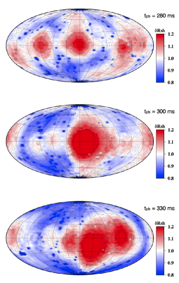
Figure 11.— Mollweide map of shock radius deviation from an average for the rotating model ($L_{\nu,52}=2.5$, $\Omega_{0}=0.1\pi$). The degree of the deviation $\delta R_{\rm sh}$ is defined as $\delta R_{\rm sh}=R_{\rm sh}(\theta,\phi)/\langle R_{\rm sh}\rangle$.

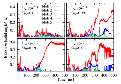
Figure 12.— Time evolution of blob sizes for four models with parameters labeled in each panel. Shown are solid angle fractions of the five largest blobs, the largest one in red and the others in different colors. The blob sizes of a non-explosion model (top left panel) are small, whereas the other explosion models have large-scale blobs.

As mentioned above, our results indicate that neutrino-driven buoyant convection is the dominant instability that triggers the onset of explosion of our parameterized 3D models. All of these models show a monotonic shock expansion after the shock reaches to a certain radius ($\sim 400$ km) and does not return later on. In this section, we discuss how rotation impacts the buoyancy-driven convection, paying particular attention to the size of buoyant bubbles as in Dolence et al. (2013), Burrows et al. (2012), Couch (2013b), Murphy et al. (2013) and Fernández et al. (2013).

As a guide to see the evolution of the buoyant bubbles, we plot in Figure 11 the deviation of the local shock position (defined as $\delta R_{\rm sh}(\theta,\phi)$) from the angle-averaged value ($R_{\rm sh}(\theta,\phi)$) for our reference rotating model. From the top panel, several protrudent blobs (red regions) can be seen around the equator at $t_{\rm pb}=280$ ms when the shock reaches an average radius of 400 km. Then, one of the high-entropy plumes (located near the center of the $4\pi$ map in the middle panel) rise all the way, locally pushing the shock ever larger radii until the global explosion is triggered (see the bottom panel). This feature was already noted by Dolence et al. (2013) and Couch (2013b) in their 3D models for non-rotating progenitors. In this work, we furthermore point out that the growth of such large-scale bubbles is easier to develop especially in the equatorial region for 3D models that include (even) moderate rotation.

For a more quantitative discussion, we plot in Figure 12 the evolution of the blob size as a function of the postbounce time. Note in the plot that each of the blob size is estimated as its solid angle measured from the center. It is clearly shown in the plot that the rotating model (top right panel) has one large blob (red line) after the shock revival ($t_{\rm pb}\gtrsim 140$-$160$ ms). On the other hand, the corresponding non-rotating model (top left panel) that fails to produce an explosion has much smaller blobs. In Figure 12, we add two more models with different input neutrino luminosity that are trending towards explosion, one is rotating (bottom left panel) and the other is non-rotating (bottom right panel). Both of these exploding models have large plumes, which continues to cover $\sim 30$-$40$ % of the whole solid angle until the globally asymmetric explosions occur.

This feature is commonly observed for models that exhibit the runaway growth of the big bubbles. When one of the blobs is stimulated by a stochastic factor such as neutrino-induced convective motion and expanding to outward, it is exposed to a small amount of accreting matter with low ram pressure. As a result, the blob expands faster and farther than the other blobs, as previously pointed out by Couch (2013b) and Fernández et al. (2013). Some models present very unique structures of the shock front, as seen in Figures 3, 4 and 5, which are far away from spherical symmetry. It is uncertain whether these characteristic structures are maintained until the shock breaks out of the stellar surface. The distorted shock front would be rounded off during the shock passage before the shock breakout or would be sharpened by nuclear energy deposition behind the shock (see Nakamura et al., 2014). To tackle with these topics, a much longer-term, better resolved 3D models covering the whole progenitor star are needed (see e.g., Kifonidis et al. (2003, 2006); Gawryszczak et al. (2010); Handy et al. (2014); Obergaulinger et al. (2014), and Kotake et al. (2012b) for a review), toward which we have attempted to make the very first step in this study.

4. CONCLUSION AND DISCUSSION

We performed a series of simplified numerical experiments to explore how rotation impacts the 3D hydrodynamics of neutrino-driven core-collapse supernovae. For the sake of our systematic study, we employed a light-bulb scheme to trigger explosions and a neutrino leakage scheme to treat deleptonization effects and neutrino losses from the PNS interior. Using a $15~{}M_{\odot}$ progenitor, we computed thirty 3D models with a suite of the initial angular momentum and the light-bulb neutrino luminosity. We find that rotation can help the onset of neutrino-driven explosions for models, in which the initial angular momentum is matched to the one obtained in recent stellar evolutionary calculations. For models with larger initial angular momentum, the PNS and the shock surface deform to be more oblate due to the larger centrifugal forces. This makes not only the gain region much more concentrated around the equatorial plane, but also the mass in the gain region bigger. As a result, hot bubbles tend to be coherently formed in the equatorial region, which pushes the shock ever larger radii until the global explosion is triggered. We found that these are the main reasons that the preferred direction of explosion in the 3D rotating models is often perpendicular to the spin axis, which is in sharp contrast to the polar explosions around the axis that was obtained in previous 2D simulations.

Finally, as a guide to discuss the strength of our parameterized explosion models, we estimate a diagnostic energy and the mass of the PNS (Figure 13). It can be seen that our rapidly rotating models (dotted lines with $\Omega_{0}=0.5\,\pi$, left panel) trending towards an energetic explosion ($\sim 10^{51}$ erg) would possibly leave behind a relatively reasonable remnant mass ($\sim 1.3$-$1.4~{}M_{\odot}$) for some particular choice of the input luminosity (e.g., dotted green line in the right panel). One has to be careful in interpreting this, because the core neutrino luminosity was assumed to be constant with time and spatially isotropic in this study. It has been shown that neutrino emission from (rapidly) rotating core is not isotropic at all (Janka & Mönchmeyer, 1989; Kotake et al., 2003; Ott et al., 2008; Brandt et al., 2011), and more importantly, the neutrino luminosity becomes smaller for models with larger initial angular momentum (Ott et al., 2008). Having admitted that the predictive power of our 3D parameterized models especially with rapid rotation is very limited, our 3D models demonstrate that even a moderate rotation ($\Omega_{0}=0.1\,\pi$) as previously thought, could significantly effect the evolution of the diagnostic energy and the remnant mass (compare solid with dashed line in Figure 13). A self-consistent 3D model (ultimately with 6D Boltzmann transport, e.g., Sumiyoshi & Yamada, 2012; Sumiyoshi et al., 2014) is apparently needed to have the final word whether rotation will or will not lead to easier onset of neutrino-driven explosions, which we are going to study as a sequel of this work (Takiwaki et al. in preparation).

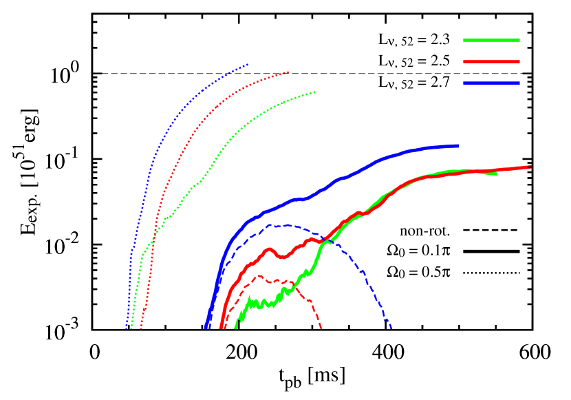
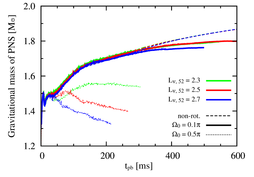
Figure 13.— Time evolution of diagnostic energy (left panel) and the mass of the PNS (defined by a fiducial density of $10^{11}~{}{\rm g}\,{\rm cm}^{-3}$) for the $L_{\nu,52}=2.3$ (green lines), $L_{\nu,52}=2.5$ (red), and $2.7$ (blue) models with different initial rotation rates. For these three values of $L_{\nu,52}$, non-rotating models (dashed lines) do not explode within our simulation time, while moderately rotating (solid) and rapidly-rotating (dotted) models are trending towards explosion. As a reference, horizontal line represents $10^{51}$ erg in the left panel.

References

- Arcones et al. (2008) Arcones, A., Martínez-Pinedo, G., O’Connor, E., et al. 2008, Phys. Rev. C, 78, 015806
- Arnett & Meakin (2011) Arnett, W. D., & Meakin, C. 2011, ApJ, 733, 78
- Bethe & Wilson (1985) Bethe, H. A., & Wilson, J. R. 1985, ApJ, 295, 14
- Bisnovatyi-Kogan et al. (1976) Bisnovatyi-Kogan, G. S., Popov, I. P., & Samokhin, A. A. 1976, Ap&SS, 41, 287
- Blondin et al. (2003) Blondin, J. M., Mezzacappa, A., & DeMarino, C. 2003, ApJ, 584, 971
- Brandt et al. (2011) Brandt, T. D., Burrows, A., Ott, C. D., & Livne, E. 2011, ApJ, 728, 8
- Bruenn et al. (2006) Bruenn, S. W., Dirk, C. J., Mezzacappa, A., et al. 2006, Journal of Physics Conference Series, 46, 393
- Bruenn et al. (2010) Bruenn, S. W., Mezzacappa, A., Hix, W. R., et al. 2010, ArXiv e-prints, arXiv:1002.4914
- Bruenn et al. (2004) Bruenn, S. W., Raley, E. A., & Mezzacappa, A. 2004, ArXiv Astrophysics e-prints, arXiv:astro-ph/0404099
- Bruenn et al. (2013) Bruenn, S. W., Mezzacappa, A., Hix, W. R., et al. 2013, ApJ, 767, L6
- Buras et al. (2006a) Buras, R., Janka, H.-T., Rampp, M., & Kifonidis, K. 2006a, A&A, 457, 281
- Buras et al. (2006b) Buras, R., Rampp, M., Janka, H.-T., & Kifonidis, K. 2006b, A&A, 447, 1049
- Burrows (2013) Burrows, A. 2013, Reviews of Modern Physics, 85, 245
- Burrows et al. (2012) Burrows, A., Dolence, J. C., & Murphy, J. W. 2012, ApJ, 759, 5
- Burrows & Goshy (1993) Burrows, A., & Goshy, J. 1993, ApJ, 416, L75+
- Burrows et al. (1995) Burrows, A., Hayes, J., & Fryxell, B. A. 1995, ApJ, 450, 830
- Couch (2013a) Couch, S. M. 2013a, ApJ, 775, 35
- Couch (2013b) —. 2013b, ApJ, 765, 29
- Dessart et al. (2006) Dessart, L., Burrows, A., Livne, E., & Ott, C. D. 2006, ApJ, 645, 534
- Dimmelmeier et al. (2002) Dimmelmeier, H., Font, J. A., & Müller, E. 2002, A&A, 393, 523
- Dimmelmeier et al. (2007) Dimmelmeier, H., Ott, C. D., Janka, H.-T., Marek, A., & Müller, E. 2007, Physical Review Letters, 98, 251101
- Dolence et al. (2013) Dolence, J. C., Burrows, A., Murphy, J. W., & Nordhaus, J. 2013, ApJ, 765, 110
- Dolence et al. (2014) Dolence, J. C., Burrows, A., & Zhang, W. 2014, ArXiv e-prints, arXiv:1403.6115
- Endeve et al. (2012) Endeve, E., Cardall, C. Y., Budiardja, R. D., et al. 2012, ApJ, 751, 26
- Endeve et al. (2010) Endeve, E., Cardall, C. Y., Budiardja, R. D., & Mezzacappa, A. 2010, ApJ, 713, 1219
- Fernández et al. (2013) Fernández, R., Mueller, B., Foglizzo, T., & Janka, H.-T. 2013, ArXiv e-prints, arXiv:1310.0469
- Fernández & Thompson (2009) Fernández, R., & Thompson, C. 2009, ApJ, 697, 1827
- Fischer et al. (2012) Fischer, T., Blaschke, D., Hempel, M., et al. 2012, Physics of Atomic Nuclei, 75, 613
- Foglizzo et al. (2006a) Foglizzo, T., Scheck, L., & Janka, H.-T. 2006a, ApJ, 652, 1436
- Foglizzo et al. (2006b) —. 2006b, ApJ, 652, 1436
- Fryer (2004) Fryer, C. L. 2004, Astrophys. J. Lett., 601, L175
- Fryer & Heger (2000) Fryer, C. L., & Heger, A. 2000, ApJ, 541, 1033
- Furusawa et al. (2013) Furusawa, S., Nagakura, H., Sumiyoshi, K., & Yamada, S. 2013, ApJ, 774, 78
- Gawryszczak et al. (2010) Gawryszczak, A., Guzman, J., Plewa, T., & Kifonidis, K. 2010, A&A, 521, A38
- Handy et al. (2014) Handy, T., Plewa, T., & Odrzywołek, A. 2014, ApJ, 783, 125
- Hanke et al. (2012) Hanke, F., Marek, A., Müller, B., & Janka, H.-T. 2012, ApJ, 755, 138
- Hanke et al. (2013) Hanke, F., Müller, B., Wongwathanarat, A., Marek, A., & Janka, H.-T. 2013, ApJ, 770, 66
- Heger et al. (2000) Heger, A., Langer, N., & Woosley, S. E. 2000, ApJ, 528, 368
- Heger et al. (2005) Heger, A., Woosley, S. E., & Spruit, H. C. 2005, ApJ, 626, 350
- Herant et al. (1994) Herant, M., Benz, W., Hix, W. R., Fryer, C. L., & Colgate, S. A. 1994, ApJ, 435, 339
- Hewish et al. (1968) Hewish, A., Bell, S. J., Pilkington, J. D. H., Scott, P. F., & Collins, R. A. 1968, Nature, 217, 709
- Huang & Gies (2006) Huang, W., & Gies, D. R. 2006, ApJ, 648, 591
- Huang & Gies (2008) —. 2008, ApJ, 683, 1045
- Iwakami et al. (2008) Iwakami, W., Kotake, K., Ohnishi, N., Yamada, S., & Sawada, K. 2008, ApJ, 678, 1207
- Iwakami et al. (2009) —. 2009, ApJ, 700, 232
- Iwakami et al. (2014) Iwakami, W., Nagakura, H., & Yamada, S. 2014, ArXiv e-prints, arXiv:1404.2646
- Janka & Müller (1996) Janka, H., & Müller, E. 1996, A&A, 306, 167
- Janka (2001) Janka, H.-T. 2001, A&A, 368, 527
- Janka (2012) —. 2012, Annual Review of Nuclear and Particle Science, 62, 407
- Janka & Mönchmeyer (1989) Janka, H.-T., & Mönchmeyer, R. 1989, A&A, 226, 69
- Keil et al. (1996) Keil, W., Janka, H.-T., & Mueller, E. 1996, ApJ, 473, L111
- Kifonidis et al. (2003) Kifonidis, K., Plewa, T., Janka, H.-T., & Müller, E. 2003, A&A, 408, 621
- Kifonidis et al. (2006) Kifonidis, K., Plewa, T., Scheck, L., Janka, H.-T., & Müller, E. 2006, A&A, 453, 661
- Kotake (2013) Kotake, K. 2013, Comptes Rendus Physique, 14, 318
- Kotake et al. (2009) Kotake, K., Iwakami, W., Ohnishi, N., & Yamada, S. 2009, ApJ, 697, L133
- Kotake et al. (2011) Kotake, K., Iwakami-Nakano, W., & Ohnishi, N. 2011, ApJ, 736, 124
- Kotake et al. (2006) Kotake, K., Sato, K., & Takahashi, K. 2006, Reports on Progress in Physics, 69, 971
- Kotake et al. (2012a) Kotake, K., Sumiyoshi, K., Yamada, S., et al. 2012a, Progress of Theoretical and Experimental Physics, 2012, 010000
- Kotake et al. (2012b) Kotake, K., Takiwaki, T., Suwa, Y., et al. 2012b, Advances in Astronomy, 2012, arXiv:1204.2330
- Kotake et al. (2003) Kotake, K., Yamada, S., & Sato, K. 2003, Phys. Rev. D, 68, 044023
- Kotake et al. (2004) Kotake, K., Yamada, S., Sato, K., et al. 2004, Phys. Rev. D, 69, 124004
- Kuroda et al. (2012) Kuroda, T., Kotake, K., & Takiwaki, T. 2012, ApJ, 755, 11
- Kuroda et al. (2014) Kuroda, T., Takiwaki, T., & Kotake, K. 2014, Phys. Rev. D, 89, 044011
- Kuroda & Umeda (2010) Kuroda, T., & Umeda, H. 2010, ApJS, 191, 439
- LeBlanc & Wilson (1970) LeBlanc, J. M., & Wilson, J. R. 1970, Astrophys. J., 161, 541
- Liebendörfer et al. (2009) Liebendörfer, M., Whitehouse, S. C., & Fischer, T. 2009, ApJ, 698, 1174
- Maeder & Meynet (2012) Maeder, A., & Meynet, G. 2012, Reviews of Modern Physics, 84, 25
- Marek & Janka (2009) Marek, A., & Janka, H.-T. 2009, Astrophys. J., 694, 664
- Marek et al. (2009) Marek, A., Janka, H.-T., & Müller, E. 2009, A&A, 496, 475
- Masada et al. (2012) Masada, Y., Takiwaki, T., Kotake, K., & Sano, T. 2012, ApJ, 759, 110
- Meakin & Arnett (2007) Meakin, C. A., & Arnett, D. 2007, ApJ, 667, 448
- Mezzacappa et al. (1998) Mezzacappa, A., Calder, A. C., Bruenn, S. W., et al. 1998, ApJ, 495, 911
- Mönchmeyer et al. (1991) Mönchmeyer, R., Schaefer, G., Mueller, E., & Kates, R. E. 1991, A&A, 246, 417
- Mösta et al. (2014) Mösta, P., Richers, S., Ott, C. D., et al. 2014, ArXiv e-prints, arXiv:1403.1230
- Müller et al. (2012) Müller, B., Janka, H.-T., & Heger, A. 2012, ApJ, 761, 72
- Müller et al. (2013) Müller, B., Janka, H.-T., & Marek, A. 2013, ApJ, 766, 43
- Müller & Hillebrandt (1979) Müller, E., & Hillebrandt, W. 1979, A&A, 80, 147
- Murphy & Burrows (2008) Murphy, J. W., & Burrows, A. 2008, ApJ, 688, 1159
- Murphy et al. (2013) Murphy, J. W., Dolence, J. C., & Burrows, A. 2013, ApJ, 771, 52
- Nakamura et al. (2014) Nakamura, K., Takiwaki, T., Kotake, K., & Nishimura, N. 2014, ApJ, 782, 91
- Nordhaus et al. (2010) Nordhaus, J., Burrows, A., Almgren, A., & Bell, J. 2010, ApJ, 720, 694
- Obergaulinger et al. (2009) Obergaulinger, M., Cerdá-Durán, P., Müller, E., & Aloy, M. A. 2009, A&A, 498, 241
- Obergaulinger et al. (2014) Obergaulinger, M., Iyudin, A. F., Müller, E., & Smoot, G. F. 2014, MNRAS, 437, 976
- Obergaulinger & Janka (2011) Obergaulinger, M., & Janka, H.-T. 2011, ArXiv e-prints, arXiv:1101.1198
- Ohnishi et al. (2006) Ohnishi, N., Kotake, K., & Yamada, S. 2006, ApJ, 641, 1018
- Ott et al. (2008) Ott, C. D., Burrows, A., Dessart, L., & Livne, E. 2008, ApJ, 685, 1069
- Ott et al. (2004) Ott, C. D., Burrows, A., Livne, E., & Walder, R. 2004, ApJ, 600, 834
- Ott et al. (2007) Ott, C. D., Dimmelmeier, H., Marek, A., et al. 2007, Physical Review Letters, 98, 261101
- Ott et al. (2012) Ott, C. D., Abdikamalov, E., O’Connor, E., et al. 2012, Phys. Rev. D, 86, 024026
- Papish et al. (2014) Papish, O., Nordhaus, J., & Soker, N. 2014, ArXiv e-prints, arXiv:1402.4362
- Rosswog & Liebendörfer (2003) Rosswog, S., & Liebendörfer, M. 2003, MNRAS, 342, 673
- Sagert et al. (2009) Sagert, I., Fischer, T., Hempel, M., et al. 2009, Physical Review Letters, 102, 081101
- Sawai & Yamada (2014) Sawai, H., & Yamada, S. 2014, ApJ, 784, L10
- Sawai et al. (2013) Sawai, H., Yamada, S., & Suzuki, H. 2013, ApJ, 770, L19
- Scheck et al. (2008) Scheck, L., Janka, H.-T., Foglizzo, T., & Kifonidis, K. 2008, A&A, 477, 931
- Shen et al. (1998) Shen, H., Toki, H., Oyamatsu, K., & Sumiyoshi, K. 1998, Nuclear Physics A, 637, 435
- Sumiyoshi & Röpke (2008) Sumiyoshi, K., & Röpke, G. 2008, Phys. Rev. C, 77, 055804
- Sumiyoshi et al. (2014) Sumiyoshi, K., Takiwaki, T., Matsufuru, H., & Yamada, S. 2014, ArXiv e-prints, arXiv:1403.4476
- Sumiyoshi & Yamada (2012) Sumiyoshi, K., & Yamada, S. 2012, ApJS, 199, 17
- Suwa et al. (2010) Suwa, Y., Kotake, K., Takiwaki, T., et al. 2010, PASJ, 62, L49
- Suwa et al. (2013) Suwa, Y., Takiwaki, T., Kotake, K., et al. 2013, ApJ, 764, 99
- Takiwaki et al. (2012) Takiwaki, T., Kotake, K., & Suwa, Y. 2012, ApJ, 749, 98
- Takiwaki et al. (2014) —. 2014, ApJ, 786, 83
- Thompson et al. (2005) Thompson, T. A., Quataert, E., & Burrows, A. 2005, ApJ, 620, 861
- van Belle (2012) van Belle, G. T. 2012, A&A Rev., 20, 51
- Wilson (1985) Wilson, J. R. 1985, in Numerical Astrophysics, 422–+
- Wilson & Mayle (1988) Wilson, J. R., & Mayle, R. W. 1988, Phys. Rep., 163, 63
- Woosley & Weaver (1995) Woosley, S. E., & Weaver, T. A. 1995, ApJS, 101, 181
- Yamamoto et al. (2013) Yamamoto, Y., Fujimoto, S.-i., Nagakura, H., & Yamada, S. 2013, ApJ, 771, 27
- Zwerger & Müller (1997) Zwerger, T., & Müller, E. 1997, A&A, 320, 209