Proposal for a running coupling JIMWLK equation

Abstract

In the CGC framework the initial stages of a heavy ion collision at high energy are described as “glasma” field configurations. The initial condition for these evolving fields depends, in the CGC effective theory, on a probability distribution for color charges. The energy dependence of this distribution can be calculated from the JIMWLK renormalization group equation. We discuss recent work [1] on a practical implementation of the running coupling constant in the Langevin method of solving the JIMWLK equation.

1 Introduction

The Color Glass Condensate (CGC) framework (for reviews see e.g. [2, 3]) provides a powerful effective theory for QCD at the high collision energies reached at the LHC. In the CGC picture, the most convenient choice for the basic degrees of freedom of a hadronic target are Wilson lines (path ordered exponentials of the color field), which describe the eikonal propagation of a high energy probe through the target. In the CGC, these are stochastic variables drawn from an energy-dependent probability distribution that satisfies the JIMWLK renormalization group equation. Different scattering processes are related to expectation values of various operators formed from the Wilson lines.

In phenomenological work the simplest operator, the two point function or “dipole”, can most conveniently be obtained from the Balitsky-Kovchegov (BK) equation [4, 5, 6] which, although the original derivation predates JIMWLK, can now be viewed as its mean field approximation. The inclusion of the running coupling constant in the BK equation (rcBK) [7, 8, 9] has been essential for successful phenomenological applications [10, 11, 12, 13, 14, 15, 16]. The running of the QCD coupling slows down the energy dependence of cross sections bringing it to rough agreement with HERA measurements. Since the full NLO version of the equation [17] has not been extensively applied to phenomenology (see however recent work in Ref. [18]), rcBK is currently the state of the art in phenomenological applications.

The few existing solutions [19, 20] of the JIMWLK equation with a running coupling have not used the same “Balitsky” [8] prescription commonly used with the BK equation. This is due to the need to decompose the evolution kernel into a product of two factors for the numerical solution of the JIMWLK equation. We describe here a recent proposal [1] for a form of the running coupling JIMWLK equation, given by Eqs. (7) and (8), and argue that it results in parametrically the same scale for the coupling constant as in the “Balitsky” prescription for the BK equation. Our starting point is different from Refs. [7, 8, 9], where one sets out to find the correct modification of the BK kernel, keeping the form of the BK equation otherwise intact. Here we in stead keep the functional form of the JIMWLK equation intact, with the result that the mean field BK approximation does not have the conventional form.

2 The JIMWLK equation

The equation for the probability distribution of Wilson lines can be expressed as a functional Langevin equation for the Wilson lines themselves [21],

$$\frac{\,\mathrm{d}}{\,\mathrm{d}y}V_{\mathbf{x}}=V_{\mathbf{x}}(it^{a})\left[\int_{\mathbf{z}}\varepsilon_{{\mathbf{x}},{\mathbf{z}}}^{ab,i}\;\xi_{\mathbf{z}}(y)^{b}_{i}+\sigma_{\mathbf{x}}^{a}\right].$$ (1)

Here we denote two dimensional vectors by ${\mathbf{x}},\cdots$. The coordinate arguments are written as subscripts. The Wilson line $V$ is a unitary matrix in the fundamental representation, generated by $t^{a}$ and $i=1,2$ is a transverse spatial index. The first term in Eq. (1) is proportional to a stochastic noise $\xi$ and the second one is a deterministic “drift” term. The coefficient of the noise in the stochastic term is the “square root” of the JIMWLK Hamiltonian

$$\varepsilon_{{\mathbf{x}},{\mathbf{z}}}^{ab,i}=\left(\frac{\alpha_{\mathrm{s}}}{\pi}\right)^{1/2}\;K_{{\mathbf{x}}-{\mathbf{z}}}^{i}\left[1-U_{\mathbf{x}}^{\dagger}U_{\mathbf{z}}\right]^{ab},\textnormal{ where }K^{i}_{{\mathbf{x}}-{\mathbf{z}}}=\frac{({\mathbf{x}}-{\mathbf{z}})^{i}}{({\mathbf{x}}-{\mathbf{z}})^{2}}$$ (2)

is the light cone wave function for soft gluon emission. The noise ${\boldsymbol{\xi}}=(\xi_{1}^{a}t^{a},\xi_{2}^{a}t^{a})$ is taken to be Gaussian and local in color, transverse coordinate and rapidity $y$ (evolution time) with $\langle\xi_{\mathbf{x}}(y)^{b}_{i}\rangle=0$ and $\langle\xi_{\mathbf{x}}(y)^{a}_{i}\xi_{\mathbf{y}}(y^{\prime})^{b}_{j}\rangle=\delta^{ab}\delta^{ij}\delta^{(2)}_{{\mathbf{x}}{\mathbf{y}}}\delta(y-y^{\prime}).$ Using the Langevin form one can easily derive the evolution equation for the dipole $\hat{D}_{{\mathbf{x}},{\mathbf{y}}}=\frac{1}{{N_{\mathrm{c}}}}\,\mathrm{Tr}\,V^{\dagger}_{\mathbf{x}}V_{\mathbf{y}}$ as

$$\partial_{y}\hat{D}_{{\mathbf{x}},{\mathbf{y}}}(y)=\frac{\alpha_{\mathrm{s}}{N_{\mathrm{c}}}}{2\pi^{2}}\int_{{\mathbf{z}}}\bigg{(}{\mathbf{K}}_{{\mathbf{x}}-{\mathbf{z}}}^{2}+{\mathbf{K}}_{{\mathbf{y}}-{\mathbf{z}}}^{2}-2{\mathbf{K}}_{{\mathbf{x}}-{\mathbf{z}}}\cdot{\mathbf{K}}_{{\mathbf{y}}-{\mathbf{z}}}\bigg{)}\left[\hat{D}({\mathbf{x}},{\mathbf{z}})\hat{D}({\mathbf{z}},{\mathbf{y}})-\hat{D}({\mathbf{x}},{\mathbf{y}})\right],$$ (3)

from which the BK equation is obtained by taking the expectation value and replacing $\langle\hat{D}\hat{D}\rangle\to\langle\hat{D}\rangle\langle\hat{D}\rangle$. It has been known for some time that the JIMWLK equation can be written in an explicitly left-right symmetric form [22]. The corresponding symmetric form for the Langevin equation was first written down in [1] as

$$V_{\mathbf{x}}(y+\,\mathrm{d}y)=\exp\left\{-i\frac{\sqrt{\alpha_{\mathrm{s}}\,\mathrm{d}y}}{\pi}\int_{\mathbf{z}}{\mathbf{K}}_{{\mathbf{x}}-{\mathbf{z}}}\cdot(V_{\mathbf{z}}{\boldsymbol{\xi}}_{\mathbf{z}}V^{\dagger}_{\mathbf{z}})\right\}V_{\mathbf{x}}\exp\left\{i\frac{\sqrt{\alpha_{\mathrm{s}}\,\mathrm{d}y}}{\pi}\int_{\mathbf{z}}{\mathbf{K}}_{{\mathbf{x}}-{\mathbf{z}}}\cdot{\boldsymbol{\xi}}_{\mathbf{z}}\right\},$$ (4)

and greatly simplifies the numerical solution of the equation due to the absence of the drift term.

3 The scale of the coupling

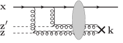
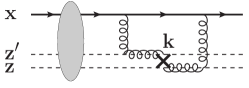
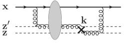
Figure 1: Virtual diagrams with coupling constant scale depending on the momentum of the gluon after the shockwave. Left: two $\xi$’s from the left of the Wilson line in Eq. (7) transported through the target (factors $V_{\mathbf{z}}$) and contracted. Center: contraction of one $\xi$ from the left and one from the right. Right: contraction of to $\xi$’s on the right.

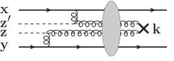
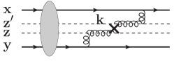
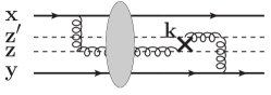
Figure 2: Real diagrams with coupling constant scale depending on the momentum of the gluon after the shockwave.

The rapidity evolution of a general correlator of $n$ Wilson lines is obtained by changing all the Wilson lines by Eq. (4), developing to order ${\boldsymbol{\xi}}^{2}$ (i.e. to order $\,\mathrm{d}y$) and taking the expectation values with the probability distribution of the noise ${\boldsymbol{\xi}}$. Physically keeping only the quadratic order in ${\boldsymbol{\xi}}$ corresponds to the fact that JIMWLK is a LO evolution equation, derived by considering the emission of only one gluon. The interpretation of the contractions between two ${\boldsymbol{\xi}}$’s is that one corresponds to the emission of a gluon in the amplitude and the other one in the complex conjugate. In the formulation that includes the deterministic term this interpretation is not as straightforward, since in Eq. (1) one is summing a noise term corresponding to a gluon emission amplitude and the deterministic term which is an emission probability, i.e. amplitude squared.

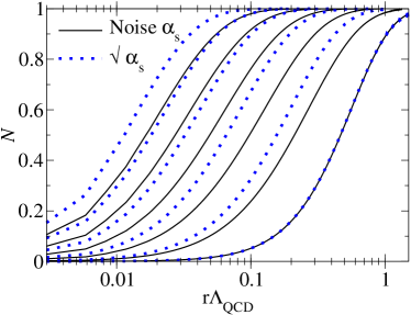
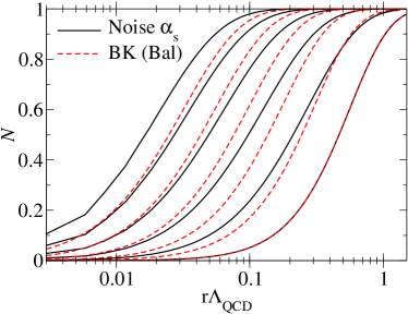
Figure 3: Left: the dipole operator evolved with Eq. (7) compared to the “square root” prescription used in [19, 20]. Both evolutions are started from the same initial condition (curves on the right). Right: comparison between Eq. (7) and the BK equation with the “Balitsky” prescription.

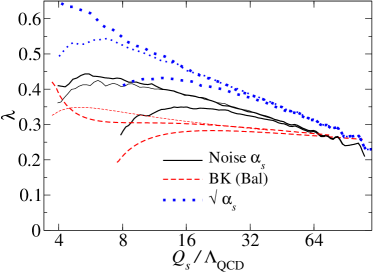
Figure 4: Evolution speed as defined in Eq. (10). The thin line uses a different regularization of the Landau pole.

Now ${\boldsymbol{\xi}}_{\mathbf{u}}$ corresponds to the emission of a gluon at coordinate ${\mathbf{u}}$ and the contraction with another ${\boldsymbol{\xi}}_{\mathbf{v}}$ is interpreted as the absorption of the same gluon, the delta function in the ${\boldsymbol{\xi}}{\boldsymbol{\xi}}$-correlator is a result of a a sum over transverse momenta of the gluon:

$$\delta^{2}({\mathbf{u}}-{\mathbf{v}})=\int\frac{\,\mathrm{d}^{2}{\mathbf{k}}}{(2\pi)^{2}}e^{i{\mathbf{k}}\cdot({\mathbf{u}}-{\mathbf{v}})}.$$ (5)

This interpretation breaks the explicit left-right symmetry by choosing to measure the gluon momentum before or after the interaction with the shockwave, i.e. on the left or right of the Wilson line in Eq. (4). Figure 1 demonstrates the three possible two point contractions in between the ${\boldsymbol{\xi}}$’s in the virtual contributions (corrections to one Wilson line at ${\mathbf{x}}$) and Fig. 2 the corresponding real contributions (contractions between ${\boldsymbol{\xi}}$’s of two Wilson lines at ${\mathbf{x}}$ and ${\mathbf{y}}$).

We will then rely on the general argument that the natural momentum scale for the running coupling is provided by the momentum of the emitted gluon. This leads directly to our proposal for implementing the running coupling in the JIWMLK equation, which is to regard the coupling constant as a property of the correlator of the noise. We then propose to simply replace $\xi$ by a new noise ${\boldsymbol{\eta}}=(\eta_{1}^{a}t^{a},\eta_{2}^{a}t^{a})$ with

$$\alpha_{\mathrm{s}}\left\langle\xi_{\mathbf{x}}^{a,i}\xi_{\mathbf{y}}^{b,j}\right\rangle=\delta^{ab}\alpha_{\mathrm{s}}\delta^{ij}\int\frac{\,\mathrm{d}^{2}{\mathbf{k}}}{(2\pi)^{2}}e^{i{\mathbf{k}}\cdot({\mathbf{x}}-{\mathbf{y}})}\longrightarrow\left\langle\eta_{\mathbf{x}}^{a,i}\eta_{\mathbf{y}}^{b,j}\right\rangle=\delta^{ab}\delta^{ij}\int\frac{\,\mathrm{d}^{2}{\mathbf{k}}}{(2\pi)^{2}}e^{i{\mathbf{k}}\cdot({\mathbf{x}}-{\mathbf{y}})}\alpha_{\mathrm{s}}({\mathbf{k}}),$$ (6)

in terms of which the rapidity step of the Wilson line is now

$$V_{{\mathbf{x}}}(y+\,\mathrm{d}y)=\exp\left\{-i\frac{\sqrt{\,\mathrm{d}y}}{\pi}\int_{\mathbf{u}}{\mathbf{K}}_{{\mathbf{x}}-{\mathbf{u}}}\cdot(V_{{\mathbf{u}}}{\boldsymbol{\eta}}_{{\mathbf{u}}}V^{\dagger}_{{\mathbf{u}}})\right\}V_{{\mathbf{x}}}\exp\left\{i\frac{\sqrt{\,\mathrm{d}y}}{\pi}\int_{\mathbf{v}}{\mathbf{K}}_{{\mathbf{x}}-{\mathbf{v}}}\cdot{\boldsymbol{\eta}}_{{\mathbf{v}}}\right\}.$$ (7)

Implementing the correlator (6) induces only a minor modification to the numerical algorithm [23] used to solve the JIMWLK equation. We denote the new noise correlator by

$${\widetilde{\alpha}}_{{\mathbf{x}}-{\mathbf{y}}}\equiv\int\frac{\,\mathrm{d}^{2}{\mathbf{k}}}{(2\pi)^{2}}e^{i{\mathbf{k}}\cdot({\mathbf{x}}-{\mathbf{y}})}\alpha_{\mathrm{s}}({\mathbf{k}}),$$ (8)

emphasizing that ${\widetilde{\alpha}}_{{\mathbf{x}}-{\mathbf{y}}}$ is not the coupling evaluated at the scale $1/|{\mathbf{x}}-{\mathbf{y}}|$, but indeed the Fourier transform of $\alpha_{\mathrm{s}}({\mathbf{k}})$. Since $\alpha_{\mathrm{s}}(k_{T})$ is a smooth, logarithmic function of $k_{T}$, ${\widetilde{\alpha}}_{{\mathbf{x}}-{\mathbf{y}}}$ is very sharply peaked around ${\mathbf{x}}={\mathbf{y}}$.

The proposed JIMWLK equation then results in the follosing evolution equation for the dipole:

$$\partial_{y}\hat{D}_{{\mathbf{x}}-{\mathbf{y}}}(y)=\frac{{N_{\mathrm{c}}}}{2\pi^{2}}\int_{{\mathbf{u}},{\mathbf{v}}}{\widetilde{\alpha}}_{{\mathbf{u}}-{\mathbf{v}}}\Bigg{\{}\left({\mathbf{K}}_{{\mathbf{x}}-{\mathbf{u}}}\cdot{\mathbf{K}}_{{\mathbf{x}}-{\mathbf{v}}}+{\mathbf{K}}_{{\mathbf{y}}-{\mathbf{u}}}\cdot{\mathbf{K}}_{{\mathbf{y}}-{\mathbf{v}}}-2{\mathbf{K}}_{{\mathbf{x}}-{\mathbf{u}}}\cdot{\mathbf{K}}_{{\mathbf{y}}-{\mathbf{v}}}\right)\frac{1}{2}\left[\hat{D}_{{\mathbf{x}},{\mathbf{u}}}\hat{D}_{{\mathbf{u}},{\mathbf{y}}}+\hat{D}_{{\mathbf{x}},{\mathbf{v}}}\hat{D}_{{\mathbf{v}},{\mathbf{y}}}-\hat{D}_{{\mathbf{x}},{\mathbf{y}}}-\hat{D}_{{\mathbf{v}},{\mathbf{u}}}\hat{Q}_{{\mathbf{x}},{\mathbf{v}},{\mathbf{u}},{\mathbf{y}}}\right],$$ (9)

involving also the quadrupole $\hat{Q}_{{\mathbf{x}},{\mathbf{v}},{\mathbf{u}},{\mathbf{y}}}=\frac{1}{{N_{\mathrm{c}}}}\,\mathrm{Tr}\,V^{\dagger}_{\mathbf{x}}V_{\mathbf{y}}V^{\dagger}_{\mathbf{u}}V_{\mathbf{v}}$. The integrand reduces to that of Eq. (3) in the limit ${\mathbf{u}}={\mathbf{v}}$.

4 Effect on the evolution

We have shown in Ref. [1] that parametrically the scale of the running coupling in Eq. (9) is the same as the “Balitsky” prescription, namely the size of smallest dipole in the problem. Figure 3 shows the result of a numerical study of these different evolution equations. It is seen that the evolution is indeed slower than with the previous “square root” coupling, and thus in better agreement with HERA data. It is, however, not quite as slow as the BK equation with the “Balitsky” prescription.

The effect of the running coupling prescription on the evolution speed, parametrized by

$$\lambda\equiv\frac{\,\mathrm{d}\ln Q_{\mathrm{s}}^{2}}{\,\mathrm{d}y}$$ (10)

is shown in Fig. 4, where the above ordering is more explicit. Initially the evolution speed depends on the initial condition, and for very small values of $Q_{\mathrm{s}}/\Lambda_{\mathrm{QCD}}$ on the regularization of the Landau pole, while at large values of $Q_{\mathrm{s}}$ lattice cutoff effects slow down the evolution in the JIMWLK case.

This work has been supported by the Academy of Finland, projects 133005, 267321 and 273464 and by computing resources from CSC – IT Center for Science in Espoo, Finland.

References

- [1] T. Lappi and H. Mäntysaari, Eur. Phys. J. C73, 2307 (2013), [arXiv:1212.4825 [hep-ph]].
- [2] F. Gelis, E. Iancu, J. Jalilian-Marian and R. Venugopalan, Ann. Rev. Nucl. Part. Sci. 60, 463 (2010), [arXiv:1002.0333 [hep-ph]].
- [3] T. Lappi, Int. J. Mod. Phys. E20, 1 (2011), [arXiv:1003.1852 [hep-ph]].
- [4] I. Balitsky, Nucl. Phys. B463, 99 (1996), [arXiv:hep-ph/9509348].
- [5] Y. V. Kovchegov, Phys. Rev. D60, 034008 (1999), [arXiv:hep-ph/9901281].
- [6] Y. V. Kovchegov, Phys. Rev. D61, 074018 (2000), [arXiv:hep-ph/9905214].
- [7] Y. V. Kovchegov and H. Weigert, Nucl. Phys. A784, 188 (2007), [arXiv:hep-ph/0609090].
- [8] I. Balitsky, Phys. Rev. D75, 014001 (2007), [arXiv:hep-ph/0609105].
- [9] J. L. Albacete and Y. V. Kovchegov, Phys. Rev. D75, 125021 (2007), [arXiv:0704.0612 [hep-ph]].
- [10] J. L. Albacete, N. Armesto, J. G. Milhano and C. A. Salgado, Phys. Rev. D80, 034031 (2009), [arXiv:0902.1112 [hep-ph]].
- [11] J. L. Albacete, N. Armesto, J. G. Milhano, P. Quiroga-Arias and C. A. Salgado, Eur. Phys. J. C71, 1705 (2011), [arXiv:1012.4408 [hep-ph]].
- [12] J. L. Albacete and C. Marquet, Phys. Lett. B687, 174 (2010), [arXiv:1001.1378 [hep-ph]].
- [13] J. Kuokkanen, K. Rummukainen and H. Weigert, Nucl. Phys. A875, 29 (2012), [arXiv:1108.1867 [hep-ph]].
- [14] J. L. Albacete, A. Dumitru, H. Fujii and Y. Nara, Nucl. Phys. A897, 1 (2013), [arXiv:1209.2001 [hep-ph]].
- [15] T. Lappi and H. Mäntysaari, Nucl. Phys. A908, 51 (2013), [arXiv:1209.2853 [hep-ph]].
- [16] T. Lappi and H. M ntysaari, Phys.Rev. D88, 114020 (2013), [arXiv:1309.6963 [hep-ph]].
- [17] I. Balitsky and G. A. Chirilli, Phys. Rev. D77, 014019 (2008), [arXiv:0710.4330 [hep-ph]].
- [18] E. Avsar, A. Stasto, D. Triantafyllopoulos and D. Zaslavsky, JHEP 1110, 138 (2011), [arXiv:1107.1252 [hep-ph]].
- [19] T. Lappi, Phys. Lett. B703, 325 (2011), [arXiv:1105.5511 [hep-ph]].
- [20] A. Dumitru, J. Jalilian-Marian, T. Lappi, B. Schenke and R. Venugopalan, Phys. Lett. B706, 219 (2011), [arXiv:1108.4764 [hep-ph]].
- [21] J.-P. Blaizot, E. Iancu and H. Weigert, Nucl. Phys. A713, 441 (2003), [arXiv:hep-ph/0206279 [hep-ph]].
- [22] A. Kovner and M. Lublinsky, JHEP 0503, 001 (2005), [arXiv:hep-ph/0502071 [hep-ph]].
- [23] K. Rummukainen and H. Weigert, Nucl. Phys. A739, 183 (2004), [arXiv:hep-ph/0309306 [hep-ph]].