Bias Correction in Species Distribution Models: Pooling Survey and Collection Data for Multiple Species

Abstract

1. Presence-only records may provide data on the distributions of rare species, but commonly suffer from large, unknown biases due to their typically haphazard collection schemes. Presence-absence or count data collected in systematic, planned surveys are more reliable but typically less abundant.

2. We proposed a probabilistic model to allow for joint analysis of presence-only and survey data to exploit their complementary strengths. Our method pools presence-only and presence-absence data for many species and maximizes a joint likelihood, simultaneously estimating and adjusting for the sampling bias affecting the presence-only data. By assuming that the sampling bias is the same for all species, we can borrow strength across species to efficiently estimate the bias and improve our inference from presence-only data.

3. We evaluate our model’s performance on data for 36 eucalypt species in southeastern Australia. We find that presence-only records exhibit a strong sampling bias toward the coast and toward Sydney, the largest city. Our data-pooling technique substantially improves the out-of-sample predictive performance of our model when the amount of available presence-absence data for a given species is scarce.

4. If we have only presence-only data and no presence-absence data for a given species, but both types of data for several other species that suffer from the same spatial sampling bias, then our method can obtain an unbiased estimate of the first species’ geographic range.

1 Introduction

Presence-only data sets (Pearce and Boyce, 2006) are key sources of information about factors that influence the habitat relationships and distributions of plants and animals, and analyzing them accurately is crucial for successful wildlife management policy. Examples include specimen collection data from museums and herbaria, and atlas records maintained by government agencies and non-government organizations. Often, these are the most abundant and freely available data on species occurrence. However, sampling bias often confounds efforts to reconstruct species distributions.

Recent work has shown that several of the most popular methods for species distribution modeling with presence-only data are equivalent or nearly equivalent to each other, and may be motivated by an underlying inhomogeneous Poisson process (IPP) model (Aarts et al., 2012; Warton and Shepherd, 2010; Renner and Warton, 2013; Fithian and Hastie, 2013). In effect, all of these methods estimate the distribution of species sightings (i.e. of presence-only records) under an exponential family model for the species distribution (Fithian and Hastie, 2013). Because presence-only data are commonly collected opportunistically, the sightings distribution is typically biased toward regions more frequented by whoever is collecting the data. Thus, it may be a poor proxy for the distribution of all organisms of that species, sighted or unsighted.

Presence-absence and other data sets collected via systematic surveys do not typically suffer from such bias. Even if (say) survey sites cluster near a major city, the data will contain more presences and more absences there. Unfortunately, if the species under study is rare, presence-absence data may carry little information about its species distribution. In this article we consider a large presence-absence data set on eucalypts in southeastern Australia. Although there are over 32,000 sites, 4 of the 36 species we consider are present in fewer than 20 of the survey sites. Presence-only data for rare species, suitably adjusted for bias, can supplement survey data.

We propose a natural extension of the IPP model for single-species presence-only data, with a view toward estimating and adjusting for sampling bias. In particular, our method brings other sources of data — presence-only and presence-absence data for multiple species — to bear on the problem, by incorporating them into a single joint probabilistic model to estimate and adjust for the bias. Some of the most popular approaches to analysis of presence-absence or presence-only data for one species are special cases of our joint approach. We evaluate our model using both presence only and presence-absence data for a set of eucalypt species from southeastern Australia. An R package implementing our method, multispeciesPP, is available in the public github repository wfithian/multispeciesPP.

1.1 The Inhomogeneous Poisson Process Model

The starting point for our model is the random set $\mathcal{S}$ of point locations of all individuals of a given species in some geographic domain $\mathcal{D}$. In spatial statistics, such a random set is called a point process, and we will call the set $\mathcal{S}$ the species process. Typically $\mathcal{D}$ is a bounded two-dimensional region.

The IPP model is a probabilistic model for the random set $\mathcal{S}=\{s_{i}\}\subseteq\mathcal{D}$. It is characterized by an intensity function $\lambda(s)$, which maps sites in $\mathcal{D}$ to non-negative real numbers. Informally, $\lambda(s)$ quantifies how many $s_{i}$ are likely to occur near $s$.

For any sub-region $A$ within $\mathcal{D}$, let $N_{\mathcal{S}}(A)$ denote the number of points $s_{i}\in\mathcal{S}$ falling into $A$. If $\mathcal{S}$ is an IPP with intensity $\lambda$, then $N_{\mathcal{S}}(A)$ is a Poisson random variable with mean

$$\Lambda(A)=\int_{A}\lambda(s)\,ds.$$ (1)

For non-overlapping sub-regions $A$ and $B$, $N_{\mathcal{S}}(A)$ and $N_{\mathcal{S}}(B)$ are independent.

If $A$ is a quadrat centered at $s$, small enough that $\lambda$ is nearly constant over $A$, then $\Lambda(A)\approx\lambda(s)|A|$, where $|A|$ represents the area of sub-region $A$. Therefore, the intensity $\lambda(s)$ represents the expected species count per unit area near $s$. The integral $\Lambda(\mathcal{D})$ over the entire study region is the expectation of $N_{\mathcal{S}}(\mathcal{D})$, the population size.

We can normalize $\lambda(s)$ to obtain the function ${p_{\lambda}(s)=\frac{1}{\Lambda(\mathcal{D})}\lambda(s)}$, which integrates to one and represents the probability distribution of individuals. An IPP may be defined equivalently as an independent random sample from $p_{\lambda}(s)$ whose size $N_{\mathcal{S}}(\mathcal{D})$ is itself a Poisson random variable with mean $\Lambda(\mathcal{D})$. Conditional on the number $N_{\mathcal{S}}(\mathcal{D})$ of points, their locations $s_{1},\ldots,s_{N_{\mathcal{S}}(\mathcal{D})}$ are independent and identically distributed (i.i.d.) draws from $p_{\lambda}(s)$. We call the intensity $\lambda(s)$ of $\mathcal{S}$ the species intensity and the density function $p_{\lambda}(s)$ the species distribution. See Cressie (1993) for a more in-depth discussion of Poisson processes and other point process models.

The first panel of Figure 1 shows a realization of a simulated IPP on a rectangular domain. The background coloring shows the intensity, and the black circles denote the $s_{i}\in\mathcal{S}$. Relatively more of the black circles occur in the green region where the intensity is highest.

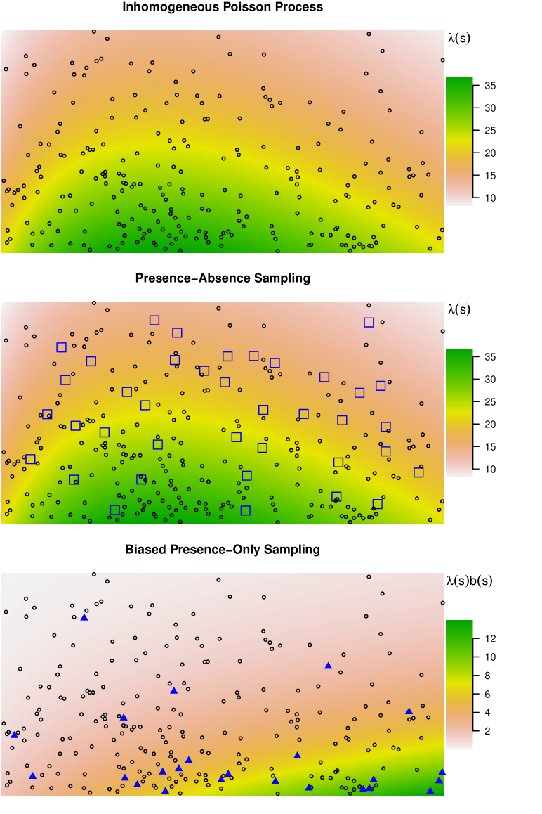
Figure 1: A Poisson process with two different sampling schemes representing our models for presence-absence and presence-only data. The top panel represents the species process against a heat map of the species intensity $\lambda(s)$. The second panel depicts presence-absence or other systematic survey methods: quadrats (blue squares) are surveyed and organisms counted in each one. The third panel depicts biased presence-only sampling, with the blue triangles indicating the presence-only process, a small and unrepresentative subset of the species process. The heat map shows the presence-only intensity ${\lambda(s)\cdot b(s)}$.

In modern ecological data sets each site in the domain has associated environmental covariates $x(s)$ measured in the field, by satellite, or on biophysical maps. These are assumed to drive the intensity $\lambda(s)$. It is convenient to model the intensity using a log-linear form for its dependence on the features:

$$\log\lambda(s)=\alpha+\beta^{\prime}x(s)$$ (2)

The linear assumption in (2) is not nearly as restrictive as it might at first seem. The feature vector $x(s)$ could contain basis expansions such as interactions or spline terms allowing us to fit highly nonlinear functions of the raw features (see, e.g., Hastie et al. (2009)).

Unfortunately, we cannot observe the entire species process $\mathcal{S}$, but we can glimpse it incompletely in various ways. The most straightforward and reliable way to learn about $\mathcal{S}$ is with presence-absence or count sampling via systematic surveys, as depicted in the second panel of Figure 1. In survey data, an ecologist visits numerous quadrats $A_{i}$ throughout $\mathcal{D}$ (the blue squares) and records the species’ occurrence or count $N_{\mathcal{S}}(A_{i})$ at each one.

Presence-only data is a less reliable but often more abundant source of information about $\mathcal{S}$. We discuss our model for presence-only data in the next section.

1.2 Thinned Poisson Processes

The presence-only process $\mathcal{T}$ comprises the set of all individuals observed by opportunistic presence-only sampling. Assuming they are identified correctly (not always a given), $\mathcal{T}$ is the subset of $\mathcal{S}$ that remains after the unobserved individuals are removed — or thinned, in statistical language.

We propose a simple model for how $\mathcal{T}$ arises given $\mathcal{S}$: an individual at location $s_{i}\in\mathcal{S}$ is included in $\mathcal{T}$ (is observed) with probability $b(s_{i})\in[0,1]$, independently of all other individuals. The function $b(s)$, which we call the sampling bias, represents the expected fraction (typically small) of all organisms near location $s$ that are counted in the presence-only data. As a result of the biased thinning, individuals in areas with relatively large $b(s)$ will tend to be over-represented relative to areas with small $b(s)$.

It can be shown that marginally

$$\mathcal{T}\sim\text{IPP}(\lambda(s)\;b(s))$$ (3)

For a formal proof, see Cressie (1993) section 8.5.6, p. 689. Informally, a small sub-region $A$ centered at $s$ contains on average $|A|\lambda(s)$ individuals, of which on average $|A|\lambda(s)\;b(s)$ are observed. If two sites $s_{1}$ and $s_{2}$ have the same intensity $\lambda(s_{1})=\lambda(s_{2})$, but $b(s_{1})=2b(s_{2})$, then (3) means the presence-only data will have about twice as many records near $s_{1}$ as $s_{2}$.

The third panel of Figure 1 displays a thinning of the Poisson process shown in the first two panels. The thinned process $\mathcal{T}$, consisting of the solid blue triangles, is shown against a heat map of the biased intensity $\lambda(s)\;b(s)$.

Sampling bias in presence-only data is not a subtle phenomenon. By our estimates in Section 4, $b(s)$ ranges from about $3\times 10^{-3}$ near Sydney to about $3\times 10^{-7}$ in the more rugged inland areas of southeastern Australia — a dynamic range of 10,000.

Some of the most popular methods for analyzing presence-only data are based explicitly or implicitly on fitting a log-linear IPP model for the process $\mathcal{T}$. It is clear from (3) that this approach effectively yields an estimate of the presence-only intensity $\lambda(s)\;b(s)$ and not the species intensity $\lambda(s)$. These estimates may be dramatically inaccurate if treated as estimates of the species intensity or species distribution.

In the case of presence-only data, $b(s)$ typically depends on the behavior of whoever is collecting the presence-only data. When sampling bias is thought to depend mainly on a few measured covariates $z(s)$ (such as distance from a road network or a large city), several authors have proposed modeling presence-only data directly as a thinned Poisson process (Chakraborty et al., 2011; Fithian and Hastie, 2013; Warton et al., 2013; Hefley et al., 2013b). A similar method was proposed in Dudık et al. (2005) in the context of the Maxent method, and Zaniewski et al. (2002) similarly propose weighting background points in presence-background GAMs according to a model for their likelihood of appearing as absences in presence-absence data.

If both $\lambda$ and $b$ are modeled as log-linear in their respective covariates, then we have

$$\log\left(\lambda(s)\;b(s)\right)=\alpha+\beta^{\prime}x(s)+\gamma+\delta^{\prime}z(s)$$ (4)

Modeling the bias as above amounts to estimating the effects of the variables $x(s)$ in a generalized linear model (GLM) for the Poisson process $\mathcal{T}$, while adjusting for control variables $z(s)$. We will refer to it as the “regression adjustment” strategy.

1.3 Identifiability, Abundance, and the Role of $\gamma$

Modeling presence-only data as a thinned Poisson process as in (4) sheds light on why it is so difficult to obtain useful estimates of presence probabilities: at best, presence-only data reflect relative intensities and not properly calibrated probabilities of occurrence. If the covariates comprising $x$ and $z$ are distinct and have no perfect linear dependencies on one other, then $\beta$, $\delta$, and the sum $\alpha+\gamma$ are identifiable, but individually $\alpha$ and $\gamma$ are not.

To see why, consider

1. a presence-only process governed by species process parameters $(\alpha,\beta)$ and thinning parameters $(\gamma,\delta)$, and

2. an alternative process with $\alpha$ replaced by ${\tilde{\alpha}=\alpha+\log 2}$ (trees are twice as abundant overall) and $\gamma$ replaced by ${\tilde{\gamma}=\gamma-\log 2}$ (the chance of observing any given tree is halved overall).

(4) means that the probability distribution of the thinned process $\mathcal{T}$ is identical in these two cases. Therefore, no matter how much data we collect, we can never distinguish parameters $(\alpha,\beta,\gamma,\delta)$ from $\left(\tilde{\alpha},\beta,\tilde{\gamma},\delta\right)$ on the basis of presence-only data alone.

Because $\beta$ is identifiable, we can use presence-only data alone to obtain an estimate for $\lambda(s)$ up to the unknown proportionality constant $e^{\alpha}$; in other words, we can estimate the species distribution $p_{\lambda}$ but not the species intensity $\lambda$. If the model is correctly specified, then likelihood estimation gives an asymptotically unbiased estimate of the model’s parameters (see e.g. Lehmann and Casella, 1998).

The species intensity $\lambda(s)$ is the product of the species distribution $p_{\lambda}(s)$ and the overall abundance $\Lambda(\mathcal{D})$. Predicting the probability that a species is present in some new quadrat $A$ requires information about both. Considerable attention has focused on whether or not we can obtain plausible estimates of abundance or of presence probabilities based on presence-only data alone. Methods like Maxent and presence-background logistic regression explicitly estimate $p_{\lambda}(s)$, but require an externally-given specification of the overall abundance if presence probabilities are required (for example, Maxent’s “logistic output,” see Elith et al., 2011). Other methods attempt to estimate presence probabilities (Lele and Keim, 2006; Royle et al., 2012), but estimates can be highly variable and non-robust to minor misspecifications of the modeling assumptions (Ward et al., 2009; Hastie and Fithian, 2013).

One of the purported advantages of the IPP as a model for presence-only data is that it does yield an estimate of overall abundance because its intercept term is identifiable (Renner and Warton, 2013). However, Fithian and Hastie (2013) show that the maximum likelihood estimate of $\widehat{\Lambda}(\mathcal{D})$ obtained from that model is exactly the number of presence-only records in the data set, so it should not be regarded as an estimate of the overall abundance.

1.4 Challenges for Regression Adjustment Using Presence-Only Data

Regression adjustment works best when the control variables $z(s)$ are not too correlated with $x(s)$, the covariates of interest. If e.g. $x_{1}(s)$ and $z_{2}(s)$ are highly correlated, then we can increase $\beta_{1}$ and decrease $\delta_{2}$ without altering the model’s predictions much. As a result, we may need a great deal of data to distinguish the effects of $\beta_{1}$ and $\delta_{2}$, and hence to tease apart $\lambda$ and $b$.

Unfortunately, correlation between $x$ and $z$ is all too common, in part because humans respond to many of the same covariates as other species do. For example, in southeastern Australia, major population centers lie along the eastern coastline, but many important climatic variables are also correlated with distance from the coast. Figure 2 plots the mean diurnal temperature range over a region of southeastern Australia, juxtaposed against our fitted bias from the model we will fit in Section 4 using pooled data. The bias is almost perfectly confounded with temperature range, making estimation highly variable even if the model is correctly specified.

Another difficulty of regression adjustment in real-world settings is that our functional form is always misspecified. In particular, it may be difficult to obtain good features in modeling the bias. Suppose for example that $x_{1}(s)$ is highly correlated with $z_{2}(s)^{2}$, which (unbeknown to us) is an important bias covariate. If we fit our model without including $z_{2}(s)^{2}$, then the $\beta_{1}x_{1}(s)$ term may serve as a proxy for the missing quadratic effect, biasing our estimate $\hat{\beta}_{1}$.

In practice we expect there to be missing variables as well as unaccounted-for nonlinearities and interactions in our models for both the species intensities and the bias alike. We can mitigate this sort of problem by adding more basis functions to $z(s)$, but as the dimension of the model increases, the standard errors of our estimates will tend to increase along with it.

If any bias covariates coincide with $x$ variables — e.g., if rugged terrain is undersampled due to inaccessibility and has an effect on a species’ abundance — then the corresponding coordinates of $\beta$ and $\delta$ are unidentifiable no matter how much presence-only data we collect.

For all its difficulties, regression adjustment on presence-only data is often preferable to no adjustment, and may be the best option when unbiased survey data is unavailable. Still, when some components of $x$ are nearly or completely confounded by $z$, a small quantity of unbiased data can go a long way, because it may provide the only solid information to distinguish true effects from bias effects (see, e.g., Figure 3). This motivates a method that can combine both biased and unbiased data to exploit the strengths of each.

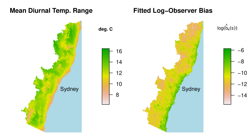
Figure 2: Mean diurnal temperature range in a coastal region of southeastern Australia, juxtaposed against our model’s fitted sampling bias. The black triangles show the locations of cities. Because most people live near the coast, sampling bias is highly correlated with distance from the coastline. Unfortunately, so are many important climatic variables. Because these variables are almost perfectly confounded with bias, it is very difficult to correct for sampling bias using presence-only data alone.

2 A Unifying Model for Presence-Absence and Presence-Only Data

The above discussion motivates a natural unifying model to explain both presence-absence and presence-only data for many species at once, which we discuss in detail here.

Assume we are equipped with a real-valued environmental covariate function $x(s)$, which takes values in $\mathbb{R}^{p}$, and bias covariate function $z(s)$, which takes values in $\mathbb{R}^{r}$. $x(s)$ and $z(s)$ represent features thought respectively to influence habitat suitably and heterogeneity in sampling effort. In general some variables may appear in both $x$ and $z$.

Let $m$ denote the total number of species for which we have data. Let $\mathcal{S}_{k}$ and $\mathcal{T}_{k}$ denote the species and presence-only processes for species $k=1,\ldots,m$. Our data set consists of two distinct types of observations for each species, presence-absence or count survey sites and presence-only sites. By modeling each of the two sampling schemes in terms of the latent species processes, we can use likelihood methods to pool data from each. We adopt the convention of indexing observations by the letter $i$, variables by the letter $j$, and species by the letter $k$.

Each observation $i$ is associated with a site $s_{i}\in\mathcal{D}$, as well as covariates $x_{i}=x(s_{i})$ and $z_{i}=z(s_{i})$. For survey sites, $s_{i}$ represents the centroid of a quadrat $A_{i}$. At survey site $i$ we observe counts $N_{ik}=N_{\mathcal{S}_{k}}(A_{i})$ or binary presence/absence indicators $y_{ik}$, with $y_{ik}=1$ if $N_{ik}>0$ and $y_{ik}=0$ otherwise.

2.1 Joint Log-Linear IPP Model for Multispecies Data

For species $k$, we propose to model $\mathcal{S}_{k}\sim\text{IPP}(\lambda_{k}(s))$, with $\mathcal{T}_{k}\sim\text{IPP}(\lambda_{k}(s)\;b_{k}(s))$ obtained by thinning $\mathcal{S}_{k}$ via $b_{k}(s)$. Both $\mathcal{S}_{k}$ and $\mathcal{T}_{k}$ are assumed to be independent across species with log-linear intensity $\lambda_{k}$ and bias $b_{k}$:

$$\log\lambda_{k}(s) =\alpha_{k}+\beta_{k}^{\prime}x(s)$$ (5)

$$\log b_{k}(s) =\gamma_{k}+\delta^{\prime}z(s).$$ (6)

Note that $\delta$ is the only model parameter not allowed to vary across species — in other words, the functions $b_{1}(s),\ldots,b_{m}(s)$ are all assumed to be proportional to one another. We call this the proportional bias assumption, and it lets us pool information across all $m$ species to jointly estimate the selection bias affecting the presence-only data. When $m$ is large, this affords us the option of working with a more expansive model for the bias term, reducing the resulting bias in our estimates for the $\alpha_{k}$ and $\beta_{k}$, which are typically of greater scientific interest.

Scientifically, the proportional-bias assumption corresponds to a belief that the biasing process has more to do with the behavior of observers than of plants and animals. Put simply, if one species is oversampled near Sydney by a factor of five relative to another region with similar features, the most likely explanation is that observers spend one fifth as much time in the second region as they do in Sydney. In that case, we should expect other species to be undersampled in the second region by roughly the same factor relative to Sydney.

The proportional-bias assumption could well be violated if, for example, most of the observers collecting samples for species 1 reside in Sydney and those collecting samples for species 2 reside in Newcastle. Even under the best of circumstances, this modeling assumption (like the other assumptions we have made) is an idealization of the truth, but it can be a very useful one if it is not too badly wrong. In Section 4 we provide evidence that the proportional bias model improves out-of-sample reconstruction of the species intensity.

We allow $\gamma_{k}$, the proportionality constant of the sampling bias, to vary by species, representing a species-dependent effect on overall sampling effort. This allows us to account for observers systematically oversampling some species relative to others. For example, if an ecologist is collecting samples in a forest, she may preferentially collect samples from rarer species. In Section 4 we give some evidence that sampling effort does indeed vary significantly by species in just this way. The cost of letting $\gamma_{k}$ vary by species is that $\alpha_{k}$ is unidentifiable unless we have some presence-absence data for species $k$. Consequently, we can estimate the species distribution $p_{\lambda}(s)$, but not the overall abundance $\Lambda(\mathcal{D})$, unless we have some presence-absence or count data for species $k$.

While our paper was in press we learned of concurrent and independent work by Giraud et al. (2014) which uses a similar Poisson thinning model to combine survey and collection data on discrete domains.

2.2 Induced Model for Survey Data

Survey data provides information about the species process $\mathcal{S}_{k}$ restricted to the survey quadrats. If the point locations of each individual within quadrat $A_{i}$ are recorded, we can directly model those locations as a log-linear IPP over the entire surveyed domain $\bigcup_{i}A_{i}$. Often we do not have access to such granular data, and only the count $N_{ik}=N_{\mathcal{S}_{k}}(A_{i})$ or presence/absence $y_{ik}$ is recorded. In such cases, the IPP model still induces a GLM likelihood for the available summary statistics $N_{ik}$ or $y_{ik}$, so that we can maximize likelihood for the available data.

If the features are continuous, then for a small quadrat $A_{i}$ the species count at the site is

$$N_{ik}=N_{\mathcal{S}_{k}}(A_{i})\approx\text{Pois}(|A_{i}|\lambda_{k}(s_{i}))=\text{Pois}\left(|A_{i}|\exp\{\alpha_{k}+\beta_{k}^{\prime}x(s_{i})\}\right).$$ (7)

Thus our joint IPP model induces a Poisson log-linear model for survey count data. The probability of $y_{ik}=1$ is

$$\mathbb{P}(N_{ik}>0)\approx 1-\exp\{-|A_{i}|\lambda_{k}(s_{i})\}=1-\exp\{-e^{\alpha_{k}+\beta_{k}^{\prime}x(s_{i})+\log|A_{i}|}\},$$ (8)

a Bernoulli GLM with complementary log-log link (McCullagh and Nelder, 1989; Baddeley et al., 2010). The complementary log-log link has been used before to study presence-absence data in ecology (e.g. Yee and Mitchell, 1991; Royle and Dorazio, 2008; Lindenmayer et al., 2009). If the expected count $\eta=|A_{i}|\lambda_{k}(s_{i})$ is very small then there is not much difference between the complementary log-log link, the logistic link, and the log link, since

$$1-\exp\{-e^{\eta}\}\approx\frac{e^{\eta}}{1+e^{\eta}}\approx e^{\eta}.$$ (9)

For simplicity assume quadrat sizes are constant and work in units where $|A_{i}|=1$. When this is not the case, $\log|A_{i}|$ enters as an offset in the GLM for observation $i$.

Importantly, we make no assumption that the survey quadrats $A_{i}$ are distributed evenly across $\mathcal{D}$ in any sense. However, our model does assume that, given the locations of $A_{i}$, the responses $y_{ik}$ for the presence-absence data are in no way impacted by $b(s)$, the sampling bias of the presence-only data.

Informally, if the $A_{i}$ tend to cluster near some population center, then we will see many presences $y_{ik}=1$ and absences $y_{ik}=0$ there, so we will not be fooled into believing the species is more prevalent there. Because we are only modeling the distribution of $y_{ik}$, the presence-absence data do not suffer from selection bias even if the geographic distribution of quadrats is very uneven.

2.3 Target Group Background Method

Phillips et al. (2009) suggested another method of using many species’ presence-only data to account for sampling bias. Using a discretization of $\mathcal{D}$ into grid cells, they propose sampling background points only from grid cells where at least one species was sighted, guaranteeing that completely inaccessible areas play no role in estimation. This method, dubbed the “target-group background” (TGB) method, can tackle sampling bias with only presence-only data, and without requiring specification of its functional form.

However, the TGB method does not distinguish between inaccessible regions and regions in which all the species are not very prevalent. Moreover, because it samples background points equally from all accessible grid cells, the TGB method does not adjust for biased sampling from one accessible region relative to another. Our method can leverage presence-absence data to directly estimate sampling bias and predict absolute prevalence. Section 4 empirically compares our method’s out-of-sample predictive performance to several competitors including the TGB method.

2.4 Maximum Likelihood Estimation

In this section we discuss estimation of our joint model. As we will see, maximum likelihood estimation amounts to fitting a very large generalized linear model to all of the data. Moreover, several familiar methods for single-species distribution modeling amount to exactly or approximately maximizing our model’s likelihood for a specific subset of our joint data set.

Because we have various sorts of observation sites $s_{i}$ we introduce notation to allow for summing over relevant subsets of them. Let $I_{\text{PA}}$ denote the set of indices $i$ for which $s_{i}$ are presence-absence survey quadrats, and let $I_{\text{PO}_{k}}$ denote the indices for presence-only sites $s_{i}\in\mathcal{S}_{k}$. Let $n_{\text{PA}}$ be the total number of survey quadrats.

For species $k$, the log-likelihood for the presence-absence data is

$$\ell_{k,\text{PA}}(\alpha_{k},\beta_{k})=\sum_{i\in I_{\text{PA}}}-y_{ik}\log\left(1-e^{-\exp\{\alpha_{k}+\beta_{k}^{\prime}x_{i}\}}\right)+(1-y_{ik})\exp\{\alpha_{k}+\beta_{k}^{\prime}x_{i}\}.$$ (10)

If $\mathbb{P}(y_{i}=1)$ is small for each quadrat, then $\ell_{k,PA}$ is very close to the log-likelihood for logistic regression on presence-absence data. In other words, applying our method to a single presence-absence data set with no other data reduces to something very close to presence-absence logistic regression for that species.

The log-likelihood for the presence-only data is

$$\ell_{k,\text{PO}_{k}} (\alpha_{k},\beta_{k},\gamma_{k},\delta)=\sum_{i\in I_{\text{PO}_{k}}}\log\left(\lambda_{k}\cdot b_{k}(s_{i})\right)-\int_{\mathcal{D}}\lambda_{k}\cdot b_{k}(s)\,ds$$ (11)

$$=\sum_{i\in I_{\text{PO}_{k}}}\left(\alpha_{k}+\beta_{k}^{\prime}x_{i}+\gamma_{k}+\delta^{\prime}z_{i}\right)-\int_{\mathcal{D}}e^{\alpha_{k}+\beta_{k}^{\prime}x_{i}+\gamma_{k}+\delta^{\prime}z_{i}}\,ds$$ (12)

In general we cannot evaluate the integral in (12) exactly. As usual, we replace the integral with a weighted sum over $n_{\text{BG}}$ background sites $s_{i}\in\mathcal{D}$. For weights $w_{i}$, we obtain the numerical approximation

$$\ell_{k,\text{PO}_{k}}(\alpha_{k},\beta_{k},\gamma_{k},\delta)\approx\sum_{i\in I_{\text{PO}_{k}}}\left(\alpha_{k}+\beta_{k}^{\prime}x_{i}+\gamma_{k}+\delta^{\prime}z_{i}\right)-\sum_{i\in I_{\text{BG}}}w_{i}e^{\alpha_{k}+\beta_{k}^{\prime}x_{i}+\gamma_{k}+\delta^{\prime}z_{i}},$$ (13)

where $I_{\text{BG}}$ are the indices corresponding to background sites. In the simplest case, the background sites are sampled uniformly from $\mathcal{D}$ and all the $w_{i}=\frac{|\mathcal{D}|}{n_{\text{BG}}}$, but other sampling schemes are possible (for a review of techniques see Renner et al., 2014). Popular procedures like Maxent and presence-background logistic regression approximately maximize (13).

Maximizing (13) for a single species $k$ with the $\gamma_{k}+\delta^{\prime}z_{i}$ terms included reduces to the regression adjustment strategy discussed in Section 1.4. If we do not include $\gamma_{k}+\delta^{\prime}z_{i}$ terms (i.e., if we assume there is no bias) we obtain the unadjusted fit (i.e. the usual fit) to the biased presence-only intensity $\lambda_{k}(s)\,b_{k}(s)$.

The presence-absence and presence-only data sets for all $m$ species together represent $2m$ independent data sets. Maximizing likelihood for all the data means maximizing the sum

$$\ell(\theta)=\sum_{k}\ell_{k,\text{PA}}(\alpha_{k},\beta_{k})+\ell_{k,\text{PO}}(\alpha_{k},\beta_{k},\gamma_{k},\delta),$$ (14)

where $\theta$ represents the full complement of coefficients

$$\theta=(\alpha_{1},\beta_{1},\gamma_{1},\ldots,\alpha_{m},\beta_{m},\gamma_{m},\delta).$$ (15)

With a bit of work we can massage the form of (14) into one large GLM in terms of a common set of $m(p+2)+r$ predictors corresponding to the entries of $\theta$. We do so by introducing auxiliary predictor variables $u_{k}$, a binary indicator that we are predicting for species $k$, and $v$, an indicator that we are predicting for presence-only instead of presence-absence data. In terms of these variables, $\alpha_{k}$ is the coefficient for $u_{k}$, $\beta_{k,j}$ for $u_{k}x_{j}$, $\gamma_{k}$ for $u_{k}v$, and $\delta_{j}$ for $vz_{j}$. More details are given in Appendix A.

The result is a very large GLM with $m(p+2)+r$ total parameters and $m(n_{\text{BG}}+n_{\text{PA}})$ total observations (one per species for each survey site and background site). Because both the number of observations and number of parameters scale linearly with $m$, the computational cost of standard approaches to estimation scales as $m^{3}p^{2}(n_{\text{BG}}+n_{\text{PA}})$.

For our eucalypt example, we have $m=36$ species, $n_{\text{BG}}=40,000$ background sites, $n_{\text{PA}}=32,612$ survey quadrats, and $p=38$ predictors (including interactions and nonlinear terms), so $m^{3}p^{2}(n_{\text{BG}}+n_{\text{PA}})\approx 5\times 10^{12}$. This is a very high computational load even for modern computers.

Fortunately, there is a great deal of structure in the design matrix, and if we exploit it properly, our computations need only scale linearly with $m$, cutting the cost by a factor of roughly $36^{2}\approx 1000$. Appendix A also details our efficient computing scheme.

2.5 Fitting Proportional Bias Models in R

As a companion to this article, we have released an R package, multispeciesPP, that can efficiently fit the models described here. The method requires formulae for the species intensity and the sampling bias, and carries out maximum likelihood as described in Section 2.4. For example, the code

mod <- multispeciesPP($\scriptstyle\mathtt{\sim}$x1 + x2, $\scriptstyle\mathtt{\sim}$z, PA=PA, PO=PO, BG=BG)

would fit a multispecies Poisson process model with presence-absence data set PA, list of presence-only data sets PO, and background data BG. The R function maximizes likelihood under the model

$$\log\lambda_{k}(s_{i}) =\alpha_{k}+\beta_{k,1}x_{i,1}+\beta_{k,2}x_{i,2}$$ (16)

$$\log b_{k}(s_{i}) =\gamma_{k}+\delta z_{i}$$ (17)

and returns fitted coefficients, and predictions.

3 Simulation

Thus far, we have discussed several distinct data sources we can bring to bear on estimating $\lambda_{k}(s)$, the intensity for the $k$th species process. A simple simulation illustrates the interplay of the different data types.

We simulate from the model (4) with covariates $(x_{1},x_{2},z)$ following a trivariate normal distribution with mean zero and covariance

$$\textrm{Cov}(x_{1},x_{2},z)=\begin{pmatrix}1&0&0.95\\ 0&1&0\\ 0.95&0&1\end{pmatrix},$$ (18)

and the coefficients for species 1 equal to:

$$(\alpha_{1},\beta_{1,1},\beta_{1,2},\gamma_{1},\delta)=(-2,1,-0.5,-4,-0.3)$$ (19)

Presence-absence data for species 1 is the most reliable reflection of $\lambda_{1}(s)$, but is available only in small quantities. Presence-only data for species 1 are abundant, but biased, as they are sampled from the intensity

$$\lambda_{1}(s)\cdot b_{1}(s)=\alpha_{1}+\beta_{1}^{\prime}x(s)+\gamma_{1}+\delta^{\prime}z(s)$$ (20)

Because $z$ is independent of $x_{1}$ but highly correlated with $x_{2}$, a presence-only data point is mainly informative about $\beta_{1,1}$ and $\beta_{1,2}+\delta$. Without supplementary data it carries almost no information about $\beta_{1,2}$ itself.

If presence-only and presence-absence data are available for many other species, then they all contribute information helping us to precisely estimate $\delta$. This makes species 1’s presence-only data much more useful: given a precise estimate of $\delta$ from other species’ data, information about $\beta_{1,2}+\delta$ is equivalent to information about $\beta_{1,2}$.

Figure 3 and the accompanying commentary shows what each data set contributes to estimating $\beta_{1,1}$ and $\beta_{1,2}$ by plotting the 95% Wald confidence ellipse for each of several models.

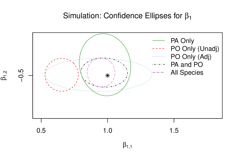
Figure 3: 95% Wald confidence regions for $\beta_{1}$, the species distribution coefficients for species 1, obtained by using five different methods. The plot illustrates the precision and accuracy with which the coefficients are estimated by each method. The black star denotes the true values of the parameters of interest. The different model types are described below:

PA data alone (Green):

The most straightforward method when PA data for species 1 is to maximize likelihood for it alone. Our estimates of both coefficients are unbiased but less precise than they could be. $z$ plays no role in the PA data or our model for it, so the precisions for the two coordinates of $\beta_{1}$ are about the same.

PO data alone, no regression adjustment (Red):

The most common use of presence-only data is to maximize likelihood using only the presence-only data for species 1, making no adjustment for sampling bias. In that case, we are effectively estimating the presence-only intensity instead of the species intensity. Here $x_{1}$ proxies for the confounding variable $z$ and $\beta_{1,2}$ is severely biased, whereas $\beta_{1,2}$ is unaffected.

PO data alone, with regression adjustment (Blue):

We can address sampling bias by attempting to estimate the effect of the confounder $z$. Our estimates are now unbiased, but $\hat{\beta}_{1,1}$ is noisy and its interval is very wide. It is quite hard to tease apart the effects of $x_{1}$ and $z$ given only PO data.

PA and PO data for species 1 (Black):

The PO data carry solid information about $\beta_{1,2}$, whereas the PA data carry the only usable information about $\beta_{1,1}$. When we combine both data sources for species 1, the precision of $\hat{\beta}_{1,2}$ roughly matches the methods using PO alone (blue and red), and the precision of $\hat{\beta}_{1,1}$ matches the method using PA alone (green).

Pooled data for all species (Purple):

We obtain the best results by pooling both presence-absence and presence-only data sets for many different species. Species $2,3,\ldots,m$ all contribute to estimating $\delta$ to high precision. As a result the presence-only data for species 1 becomes much more useful for estimating $\beta_{1,1}$, because we know how to correct for the sampling bias.

4 Eucalypt Data

We have just seen how the various sources of data can work in concert to give far more precise estimates than we could obtain from any one data set by itself. Additionally, we evaluate our model’s performance on a data set of 36 species of genera Eucalyptus, Corymbia, and Angophora in southeastern Australia.

The presence-absence data consist of 32,612 sites where all the species were surveyed, with an average of 547 presences per species. The species exhibit a great deal of variability with respect to their overall abundance, with 4 species having fewer than 20 total observations, and 8 having more than 1000.

The presence-only data consist of 764 observations on average per species, supplemented with 40,000 background points sampled uniformly at random from the study region. More information on data sources may be found in Appendix C. The rarest species in the presence-only data, Eucalyptus stenostoma, has 90 observations.

We use 15 environmental covariates in our model for the species process, allowing for nonlinear effects in 4 of them: temperature seasonality, rainfall seasonality, precipitation in June/July/August, moisture index in the lowest quarter, and annual precipitation overall. Our model for the bias includes nonlinear effects for predictors including distance to road, distance to the nearest town, distance to the coast, ruggedness, whether the locale has extant vegetation, and the number of presence-absence sites nearby. Appendix B discusses the model form in more detail.

The four panels of Figure 4 contrast our model’s fit for a single species, Eucalyptus punctata, with the fit that we would obtain by using presence-only data alone with no bias adjustment. A satellite image of the same region provided for comparison and orientation. The top left panel displays the fitted intensity we obtain by modeling E. punctata’s presence-only data as an IPP whose intensity is driven by environmental variables. We obtain an estimate of the presence-only intensity, which in this case is concentrated mostly near Sydney and the coast.

The top right and lower left panels show our model’s estimates $\hat{b}_{k}(s)$ of the bias and $\hat{\lambda}_{k}(s)$ of the species intensity. Unsurprisingly, distance from the coast, and from Sydney, are strong drivers of our model’s fitted sampling bias. In the lower left panel, the intensity is shifted significantly toward the western hinterland.

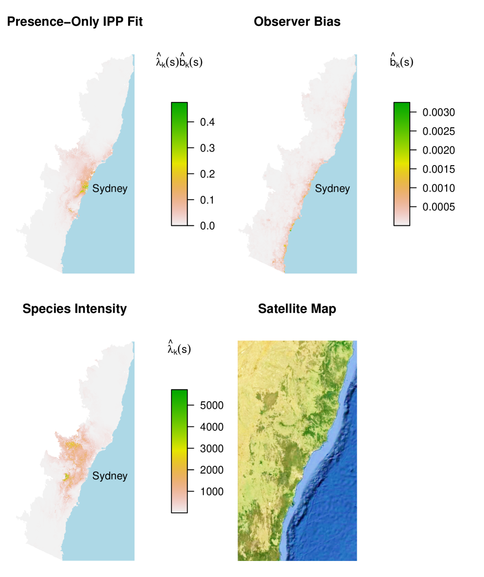
Figure 4: Model fits for Eucalyptus punctata in southeastern Australia. Top left panel: estimate of presence-only intensity in units of $1/\text{km}^{2}$, using presence-only data alone and making no adjustment for bias. Top right: fitted sampling bias $\hat{b}_{k}(s)$ in our proportional sampling bias model. Lower left: fitted species intensity $\hat{\lambda}_{k}(s)$ for our model, in units of $1/\text{km}^{2}$. Lower right: satellite image from Google Earth. In the presence-only data, many more trees were observed in near Sydney than in the western hinterland, but our model infers a higher intensity in the undersampled western region.

To evaluate our model quantitatively, we ask two questions: first, how well do the data agree with the assumption of proportional sampling bias? Second, do we obtain better predictions when pooling multiple data sets across multiple species?

4.1 Checking the Proportional Bias Assumption

We can check the proportional bias assumption within the context of our GLM. To check whether the bias coefficient corresponding to some $z_{j}$ should vary by species, we can estimate the same model as before, but now allowing that coordinate of $\delta$ to vary by species.

In terms of the large GLM described in Section 2.4, we can estimate our model as before by augmenting the design matrix with interactions between the species identifiers $u_{k}$ and the bias variable $z_{j}$. These variables then have coefficients $\delta_{k,j}$. In this model the proportional bias assumption corresponds to the null hypothesis of no interaction effects, which we can test using standard likelihood-based methods.

As usual, it is rather unlikely that the proportional bias assumption — or any other aspect of our model — holds exactly. Even if the assumption holds for some true functions $\lambda_{k}(s)$ and $b_{k}(s)$, we may still see spurious correlations when we fit a complex model using a misspecified log-linear functional form. Nevertheless, it is of interest to identify whether some interactions stand out strongly compared to the noise level, and if so how large they are.

Because of spatial autocorrelation in both the presence-absence and presence-only data, traditional likelihood-based confidence intervals for the interaction effects $\delta_{k,j}$ are likely to be anticonservative, as are bootstrap intervals based on i.i.d. resampling. To account properly for the spatial autocorrelation, we use the block bootstrap to compute confidence intervals for the coefficients (Efron and Tibshirani, 1993). We separate the landscape into a checkerboard pattern with 261 rectangular regions with sides of length 1/3-degree of longitude and latitude (approximately 31 km $\times$ 37 km at latitude $33^{\circ}$ South). In each of 400 bootstrap replicates we resample 261 whole regions with replacement.

Dependence of $\delta$ on Species:

We test our assumption explicitly for the variable “distance to coast,” which is the most important predictor of bias. The evidence in the data regarding our assumption is somewhat mixed, but on the whole it does not appear that the proportional bias model fits the data perfectly. For some species, there is sufficient evidence to reject $H_{0}$.

Figure 5 shows the 95% bootstrap confidence interval for the idiosyncratic sampling bias of Eucalyptus punctata, as a function of distance to coast. We see that, even after accounting for the overall bias that affects the other 35 species, we still have too many coastal presence-only observations of punctata. This could be linked to the fact that the punctata data are concentrated near Sydney, which is more heavily populated than other coastal regions, but with many confounding factors at play it is hard to know. Appendix B has more detailed results for more species.

If interactions like these are strong, we can allow some of the coordinates of $\delta$ to vary by $k$ and others not. There is a bias-variance tradeoff, however, since the proportional-bias assumption is what allows us to share information across species. We will see in Section 4.2 that even when the model is an imperfect fit, it can nevertheless substantially improve predictive performance on held-out presence-absence data.

Figure 5: Idiosyncratic sampling bias for E. punctata and E. dives as a function of distance to coast in km. The dashed lines show 95% block-bootstrap confidence intervals. It appears that after adjusting for the bias $\delta^{\prime}z(s)$ that is shared across all species, there is some residual bias left over for punctata. By contrast, for E. dives, there is no significant interaction. Even though the proportional sampling bias model is misspecified for E. punctata, it still substantially improves out-of-sample predictive accuracy, as we will see in Section 4.2. The corresponding curves for all the species can be found in Appendix B.

Dependence of $\gamma$ on Species:

By default, our model allows $\gamma$ to vary by species, but we need not always do so. In fact, if we assumed $\gamma$ does not vary by species, then we would only need joint presence-absence and presence-only data for one species to obtain an estimate for $\gamma$. Therefore, we could estimate abundance (and therefore presence probabilities) for every species given presence-absence and presence-only data for a single species and presence-only data for every other species.

Define relative sampling effort as the ratio

$$\rho_{k}=\frac{\exp\{\gamma_{k}\}}{\displaystyle\min_{k^{\prime}=1}^{m}\exp\{\gamma_{k^{\prime}}\}},$$ (21)

so that $\rho_{k}=1$ for all $k$ if and only if the $\gamma_{k}$ are all equal.

Figure 6 shows our model’s estimates $\hat{\rho}_{k}$, plotted against the total number of presence-absence observations. For the eucalypt data it appears that the assumption of a common $\gamma$ for every species is probably not reasonable. It appears the presence-only intercept $\gamma$ varies systematically by species, with effort being substantially higher for the rarer species. Thus, the data appear to support our decision to allow $\gamma$ to vary by species.

Figure 6: Our model’s estimate of relative sampling effort $\rho_{k}$, plotted versus the total abundance of each species, with each variable plotted on a log scale. It appears that more effort is made to sample rare species.

4.2 Predictive Evaluation of the Model

Our goal in pooling data was to supplement the presence-absence data for a given species with multiple other more abundant sources of data, to allow for more efficient estimation of the species intensity $\lambda_{k}(s)$ and its coefficients. One measure of our success is whether this data pooling actually improves predictive performance on held-out presence-absence data.

For comparison, we also estimate our joint model using a) both the presence-only and presence-absence data for species $k$, and b) presence-only and presence-absence data for all 36 species combined.

Note that in all three cases we are estimating the exact same joint model with three nested data sets:

PA data alone for species $k$:

The most natural competitor to our method is to fit the Bernoulli complementary log-log GLM model with the same predictors, but only on species $k$’s presence-absence data. This is a special case of the joint method, for which only presence-absence data are available for species $k$.

PA and PO data for species $k$:

Augmenting the presence-absence data with presence-only data for the same species improves our coefficient estimates for environmental variables that are independent of sampling bias.
When there is no presence-absence data, we are fitting the thinned Poisson process model to PO data alone. This is regression-adjusted analysis of PO data, discussed in Section 1.4.

Pooled data for all species:

Using data for all species gives better estimates of the predictors that are badly confounded by sampling bias.

In addition we introduce two more competitors that use presence-only data alone:

PO data alone for species $k$, unadjusted for bias:

Using species $k$’s presence-only data alone, and ignoring sampling bias, is the most common method for analyzing presence-only data. It estimates the presence-only intensity, and then makes predictions as though that were the same as the species intensity. This method can suffer dramatically from bias.

PO data for all species, using the TGB method:

We implement the TGB method with pixel size 9 arc seconds (the resolution level of our covariates).

Our evaluation method effectively treats the presence-absence data as a “gold standard,” unaffected by bias. This point of view may not always be reasonable, but eucalypts are relatively large and hard for surveyors to miss, so the presence-absence data probably do reflect the true presence or absence of trees in their respective quadrats, notwithstanding identification errors.

We emphasize that we are comparing the different methods with respect to their performance on held-out presence-absence data and not on held-out presence-only data. This distinction is important, because our goal is to reconstruct the species intensity and not the presence-only intensity. All three methods train on the same amount of presence-absence data for species $k$. The data-pooling methods can only beat the simpler method if the other data sets carry useful information about the species intensity of species $k$, and if our joint model effectively processes that information without biasing our estimate too badly.

We then use ten-fold block cross-validation to evaluate each method with respect to its predictive log-likelihood. Using the same rectangular regions as in Section 4.1, we randomly assign the 261 whole regions to ten folds, with each fold containing 26 random regions and the one left-over region excluded. Figure 7 shows one training-test split used for our procedure. Importantly, all data taken from the test region — presence-absence, presence-only, and background — is held out of the training set.

The gains from data pooling are greatest when the presence-absence data for a species of particular interest (say, species $k$) are either scarce or non-existent. To emulate estimation with presence-absence data sets ranging from scarce to abundant, we further downsampled the presence-absence training data for species $k$.

We fit all the models with a ridge penalty on all of the coefficients except the intercepts $\alpha$ and $\gamma$. That is, we minimize

$$\ell(\alpha,\beta,\gamma,\delta)+\frac{\nu}{2}\|\beta\|_{2}^{2}+\frac{\nu}{2}\|\delta\|_{2}^{2},$$ (22)

with penalty multiplier $\nu=100$. Penalizing the coefficients in this way is known as regularization, and it allows for efficient estimation of parameters in complex models. For more details see e.g. Hastie et al. (2009).

Figures 8 and 9 show the results of block cross-validation for two species in the data set: Eucalyptus punctata and Eucalyptus dives. Results for the other species are qualitatively similar and can be found in Appendix B. We evaluate the various methods according to two metrics of predictive performance: predictive log-likelihood (left panel) and area under the predictive ROC curve, averaged over the ten test folds (AUC, right panel). Lawson et al. (2014) contrast prevalence-dependent metrics like log-likelihood, which measure the accuracy of absolute out-of-sample presence probabilities, with prevalence-independent metrics like AUC, which depend only on the ordering of predictions.

Doing well in predictive log-likelihood requires a good estimate of the intercept $\alpha_{k}$ — i.e., of the absolute intensity $\lambda_{k}(s)$. Because $\alpha_{k}$ is confounded with $\gamma_{k}$ in presence-only data, and because $\gamma_{k}$ varies by species, the two data-pooling methods cannot estimate absolute intensities without a little presence-absence data from species $k$. By contrast, AUC only depends on estimates of relative intensity $\frac{\lambda_{k}(s)}{\Lambda_{k}(\mathcal{D})}$, which is invariant to $\hat{\alpha}_{k}$ and can be estimated with no presence-absence data for species $k$. Estimates without any presence-absence data for species $k$ are shown above the label “0” on the horizontal axis.

As we have seen in Figure 4, E. punctata suffers dramatically from sampling bias because Sydney, the largest city, lies on the eastern edge of its habitable zone. As a result, the unadjusted presence-only method performs very poorly compared to the methods that account for bias. By contrast, the habitable zone of E. dives lies mainly in the western part of the study region where the sampling bias function $\log b_{k}$ has a much gentler gradient. As a result, the unadjusted presence-only analysis does relatively well. The method that pools across all 36 species does even better: its AUC using none of E. punctata’s presence-absence data (and only the presence-absence data for the other 35 species) is indistinguishable from its AUC using all of the presence-absence data. See Appendix B for the corresponding plots for all species.

Table 1 compares the four best methods using a moderate value, 1000, for the number of non-missing presence-absence sites. Our method pooling presence-absence and presence-only data for all species performs well consistently, coming within 0.01 of the best method for all but one species. Interestingly, the TGB method performs second best despite its having no access to the presence-absence data.

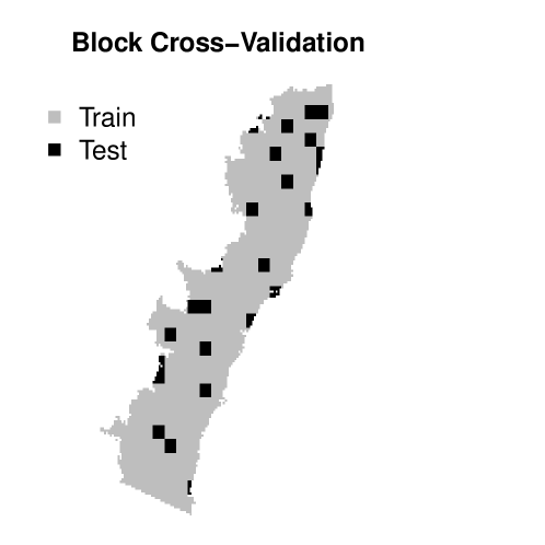
Figure 7: Depiction of our block cross-validation scheme for the eucalypt data. Entire rectangular blocks are sampled together to help account for spatial autocorrelation.

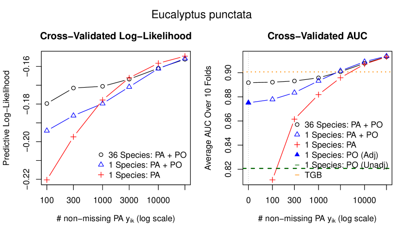
Figure 8: Block cross-validated log-likelihood and AUC for E. punctata (higher is better). Pooling data from other sources gives a substantial boost to predictive performance when the presence-absence data set is small, but only when we make an adjustment for the bias.

In the right panel, the leftmost blue triangle (“1 species: PA+PO” with no PA data), we are fitting the thinned IPP model to PO data alone. This is the regression adjustment strategy discussed in Section 1.4. Note that using presence-only data without any adjustment for bias performs quite poorly compared to the other methods. Because the habitable zone for E. punctata includes Sydney as well as more inaccessible regions to its west, ignoring the sampling bias can wreak havoc on our estimates.

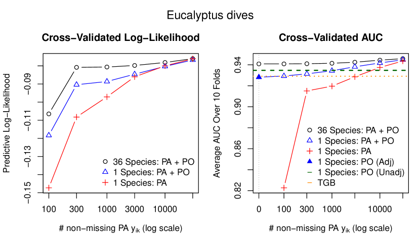
Figure 9: Block cross-validated log-likelihood and cross-valid AUC for the species E. dives (higher is better). Pooling data from other sources gives a substantial boost to predictive performance when the presence-absence data set is small. Because E. dives occurs in the southwestern part of the study region, where the bias function has a relatively gentle gradient, the sampling bias plays a less vital role.

In the right panel, the leftmost blue triangle (“1 species: PA+PO” with no PA data), we are fitting the thinned IPP model to PO data alone. This is the regression adjustment strategy discussed in Section 1.4.

	PA Only	PA + PO	PA + PO	TGB
	1 Species	1 Species	36 Species	36 Species
A. bakeri	0.893	0.915	0.932	0.933
C. eximia	0.921	0.947	0.952	0.952
C. maculata	0.783	0.778	0.785	0.742
E. agglomerata	0.801	0.834	0.820	0.808
E. blaxlandii	0.904	0.934	0.944	0.934
E. cypellocarpa	0.861	0.852	0.867	0.825
E. dalrympleana (S)	0.873	0.910	0.926	0.931
E. deanei	0.811	0.855	0.906	0.894
E. delegatensis	0.971	0.971	0.981	0.982
E. dives	0.920	0.934	0.941	0.929
E. fastigata	0.905	0.900	0.916	0.907
E. fraxinoides	0.920	0.935	0.963	0.963
E. moluccana	0.881	0.909	0.911	0.881
E. obliqua	0.870	0.914	0.918	0.906
E. pauciflora	0.874	0.897	0.928	0.928
E. pilularis	0.807	0.807	0.805	0.811
E. piperita	0.889	0.844	0.886	0.871
E. punctata	0.882	0.893	0.896	0.901
E. quadrangulata	0.835	0.843	0.840	0.823
E. robusta	0.878	0.883	0.892	0.894
E. rossii	0.957	0.966	0.965	0.962
E. sieberi	0.857	0.813	0.881	0.875
E. tricarpa	0.969	0.970	0.971	0.965

Table 1: AUC cross-validation results for all species with at least 100 presence-absence data points. The first three methods are evaluated with 1000 non-missing presence absence data points for the species under study. In each row, numbers are bolded for methods coming within 0.01 of the best method. Our method pooling presence-absence and presence-only data for all species performs well consistently, coming within 0.01 of the best method for all but one species.

5 Discussion

We have proposed a unifying Poisson process model that allows for joint analysis of presence-absence and presence-only data from many species. By sharing information, we can obtain more precise and reliable estimates of the species intensity than we could obtain from either data set by itself.

Moreover, we have seen in Section 4 that the proportional bias can be a reasonable fit for some real ecological data sets. In this data set, and we suspect in many others, sampling bias can have a major effect on fitted intensities if not appropriately accounted for.

5.1 Benefits of Data Pooling

Throughout we have focused mainly on the way that pooling presence-absence and presence-only data from many species can help address selection bias. Even when selection bias is not a major concern, data pooling can still be beneficial.

In the simplest case, presence-absence data can be fruitfully supplemented by more abundant presence-only data from the same species. In Figure 9, we see that the presence-only data for E. dives is not very biased, as evidenced by the good performance of the unadjusted fit. In this case, combining the presence-absence data with presence-only data still led to a substantial improvement in predictive performance, and combining with data from other species helped even more. In other cases, we may have presence-only data for many species but no presence-absence data. In that case, our method still provides a means for pooling data to estimate $\delta$ more efficiently.

5.2 Common Misspecifications of the IPP Model

Aside from the proportional bias assumption, we should be mindful of several other sources of misspecification. The most obvious is that our log-linear functional form is almost certainly incorrect in any given case. Three others that merit special consideration are spatial autocorrelation in the data, biased detection of presence-absence data, and spatial errors in environmental covariates and point observations.

Spatial Autocorrelation:

The Poisson process model assumes that, given the covariates for a given site, an individual is no more or less likely to occur simply because there is another individual nearby. In ecological data, this assumption is rather tenuous; for example, trees of the same species often occur together in stands; or, different species may compete with each other for resources. Renner and Warton (2013) discuss goodness-of-fit checks and present empirical evidence against the Poisson assumption. For a more general discussion of alternatives to the Poisson process model, see Cressie (1993); Gaetan and Guyon (2009).

Similarly, for systematic survey data, we should proceed with caution in modeling count data as Poisson, because actual counts may be overdispersed due to autocorrelation within a quadrat, or correlated with counts for nearby sites because of longer-range autocorrelation. When autocorrelation is present, nominal standard errors computed under the Poisson assumption can be much too small, as can i.i.d. cross-validation estimates of prediction error or i.i.d. bootstrap standard errors. Resampling methods such as the bootstrap or cross-validation can be made much more robust to autocorrelation if they resample whole blocks at a time (Efron and Tibshirani, 1993), and in Section 4 we use the block bootstrap and block cross-validation to analyze our eucalypt data set. Discussion of alternative block bootstrap procedures and choosing block size may be found in Hall et al. (1995); Nordman et al. (2007); Guan and Loh (2007).

Imperfect Detection:

Even in presence-absence and other systematic survey data, surveyors may not have the time or resources to exhaustively survey a given quadrat, and thus some organisms may be missed in the surveys.

Suppose, for example, that an organism at $s$ is detected by surveyors with probability $q(s)$. Then the count $y$ in quadrat $A$ centered at $s$ is not distributed as $\text{Pois}(\lambda(s)|A|)$, but rather as $\text{Pois}(q(s)\lambda(s)|A|)$. If $q(s)$ is constant, all our estimates of $\alpha_{k}$ will be biased downward by exactly $\log q$. This would bias estimates of abundance but not the estimated species distribution, which depends only on $\hat{\beta}_{k}$.

If $q(s)$ is a non-constant function of $s$ — e.g., if non-detection is a bigger problem in heavily forested sites — then we may incur bias for both $\alpha_{k}$ and $\beta_{k}$. If sites are visited repeatedly, then under some assumptions an estimate of non-detection may be obtained, by methods discussed in e.g. Royle and Nichols (2003); Dorazio (2012). Estimates of detection probability can sometimes be obtained without repeat observations under stronger modeling assumptions (Lele et al., 2012; Sólymos et al., 2012).

Non-detection in presence-absence data is largely analogous to the sampling bias problem for presence-only data, and we could in principle model and adjust for it using similar methods to the ones we propose for addressing biased presence-only data.

Spatial Errors

Opportunistic presence-only data may also suffer from errors in the recorded locations of point observations. Similarly, environmental covariates are often measured at a relatively coarse scale, in which case the covariates attributed to point $s_{i}$ may be inaccurate. If important environmental covariates fluctuate on a fine scale compared to the scale of these errors, the errors may lead to attenuated effect size estimates (see e.g. Graham et al., 2008). Hefley et al. (2013a) propose methods to correct for spatial errors in presence-only records.

A similar issue can arise in the analysis of presence-absence or count data, when we use the centroid of a presence-absence quadrat as a proxy for the integral $\int_{A_{i}}\lambda(s)\,ds$, which may not be appropriate if the variables fluctuate on a fine scale relative to quadrat size. In such cases, it is especially helpful to record point locations within quadrats rather than recording only presence-absence or count data summarized at the quadrat level.

5.3 Extensions

As discussed elsewhere, there are many useful ways to extend GLM fitting procedures. GAMs, gradient-boosted trees, and other forms of regularization on model parameters are all immediate extensions of the approach we have outlined here. Like other methods, our method’s results on a given data set will depend on making good choices regarding featurization and regularization.

Finally, in our approach we are forced to assume a functional form for the sampling bias, and if our model is wrong, we will not account correctly for the sampling bias. Studies quantifying patterns of sampling bias in relation to spatial covariates are currently scarce, but could help to justify a more accurate model of sampling bias than one based on intuitive selection of covariates, as applied here. Nonetheless, in future work we plan to investigate models that treat the sampling bias nonparametrically, imposing no assumptions on its functional form.

Appendix A Maximum Likelihood Estimation as a Joint GLM

Recall that maximizing likelihood for the full data set means maximizing

$$\ell(\theta)=\sum_{k}\ell_{k,\text{PA}}(\alpha_{k},\beta_{k})+\ell_{k,\text{PO}}(\alpha_{k},\beta_{k},\gamma_{k},\delta),$$ (23)

where

$$\ell_{k,\text{PA}}(\alpha_{k},\beta_{k}) =\sum_{i\in I_{\text{PA}}}-y_{ik}\log\left(1-e^{-\exp\{\alpha_{k}+\beta_{k}^{\prime}x_{i}\}}\right)+(1-y_{ik})\exp\{\alpha_{k}+\beta_{k}^{\prime}x_{i}\}$$ (24)

$$\ell_{k,\text{PO}_{k}}(\alpha_{k},\beta_{k},\gamma_{k},\delta) \approx\sum_{i\in I_{\text{PO}_{k}}}\left(\alpha_{k}+\beta_{k}^{\prime}x_{i}+\gamma_{k}+\delta^{\prime}z_{i}\right)-\sum_{i\in I_{\text{BG}}}w_{i}e^{\alpha_{k}+\beta_{k}^{\prime}x_{i}+\gamma_{k}+\delta^{\prime}z_{i}}$$ (25)

In this section we discuss how to massage (23) into a large GLM in terms of a common set of $m(p+2)+r$ predictors and coefficients. For the moment, we ignore the sum over $I_{\text{PO}_{k}}$ in (25) and deal with the other two sums. The sum in (24) is the log-likelihood for a Bernoulli GLM with complementary log-log link and the sum over $I_{\text{BG}}$ in (25) is the log-likelihood for a weighted Poisson GLM with log link.

Note that at each survey site we have $m$ presence-absence observations, one for every species. Similarly, we will introduce one “dummy” response $y_{ik}=0$ for each species $k$ at each background site $i$, for $m(n_{\text{PA}}+n_{\text{BG}})$ total observations. For observation $ik$, introduce auxiliary indicator variables

$$u_{ik_{1},k_{2}} =\left\{\begin{matrix}1&k_{1}=k_{2}\\ 0&\text{otherwise}\\ \end{matrix}\right.$$ (26)

$$v_{ik} =\left\{\begin{matrix}1&i\in I_{\text{BG}}\\ 0&\text{otherwise}\\ \end{matrix}\right.$$ (27)

The variable $u_{k}$ allows parameters to vary by species. For example, $\alpha_{k}$ is the coefficient for $u_{k}$ and $\beta_{k,j}$ is the coefficient for the interaction $x_{j}u_{k}$. The variable $v$ gives us bias terms that apply only to terms in the presence-only likelihood. Thus $\gamma_{k}$ is the coefficient for $u_{k}v$ and $\delta_{j}$ is the coefficient for $z_{j}v$.

For example, the linear predictor for count or presence-absence for species $k$ at a survey site with predictors $x$ and $z$ is

$$\alpha_{k}+\beta_{k}^{\prime}x_{i}=\sum_{1\leq h\leq m}\left(\alpha_{h}u_{ik,h}+\beta_{h}^{\prime}x_{i}u_{ik,h}+\gamma_{h}u_{ik,h}v_{ik}\right)+\delta^{\prime}z_{i}v_{ik},$$ (28)

using $v=0$ because we are predicting for presence-absence data.

To check the proportional bias assumption for variable $z_{j}$ — that is, to check the assumption that $\delta_{j}$ should be the same for every species — we can augment the model with interactions $z_{j*k}=u_{k}z_{j}$ for each $k$, and test the hypothesis that each of those variables has no effect on the regression.

Let $X_{\text{PA}}$ denote the $n_{\text{PA}}\times p$ matrix with all $x$ variables for all the survey sites, and let $X_{\text{BG}}$ and $Z_{\text{BG}}$ denote all the $x$ and $z$ variables for all the background sites. Then if

$$X=\begin{pmatrix}1&X_{\text{PA}}&0\\ 1&X_{\text{BG}}&1\end{pmatrix},\;\;\;Z=\begin{pmatrix}0\\ Z_{\text{BG}}\end{pmatrix},$$ (29)

our likelihood is a large weighted GLM with $m(n_{\text{PA}}+n_{\text{BG}})$ observations and overall design matrix

$$\mathbb{X}=\begin{pmatrix}X&0&\cdots&0&Z\\ 0&X&\cdots&0&Z\\ \vdots&\vdots&\ddots&\vdots&\vdots\\ 0&0&\cdots&X&Z\\ \end{pmatrix},\quad\text{ and coefficients }\quad\theta=\begin{pmatrix}\theta_{1}\\ \vdots\\ \theta_{m}\\ \delta\end{pmatrix}.$$ (30)

The weights are $w_{i}$ for rows corresponding to background site $i$, and 1 for presence-absence sites. Note that the response family and link function are different for different rows.

Turning to the sums over $I_{\text{PO}_{k}}$ in (25), note that they are linear in the coefficients, so all $k$ sums can be combined to obtain a single linear term of the form $\theta^{\prime}M$. All the parameters may be estimated simultaneously via a slight modification of iterative reweighted least squares that takes into account the $m$ linear terms.

A.1 Iterative Reweighted Least Squares Using Block Structure

Let $n=n_{\text{PA}}+n_{\text{BG}}$. $\mathbb{X}$ has $mn$ rows and $m(p+2)+r$ columns. In principle, we could form the matrix $\mathbb{X}$ and use standard GLM software to fit the model, but we would pay a very high computational price for estimating multiple species at a time.

The main computational bottleneck in each iteration is solving a large weighted linear least-squares problem with $mn$ equations (one per species per site) and $m(p+2)+r$ unknowns. The update for step $t$ requires solving a weighted linear least-squares problem with row weights $W^{(t)}=\textrm{diag}\left(w^{(t)}\right)$ and working responses $u^{(t)}$:

$$\min_{\theta}\left\|W^{(t)}\left(\mathbb{X}\theta-u^{(t)}\right)\right\|_{2}^{2}.$$ (31)

Solving a completely general problem of the form (31) would require $\mathcal{O}(m^{3}np^{2}+mnr^{2})$ floating point operations. Fortunately, we can store and compute much more cheaply if we exploit the special block structure of $\mathbb{X}$.

Our computational scheme relies heavily on the following well-known and highly useful lemma:

Lemma 1 (Partitioned Least Squares).

Consider the least-squares problem

$$\min_{v}\left\|(A\;\;B)\binom{v_{1}}{v_{2}}-c\right\|_{2}^{2}.$$ (32)

Let $B._{A}$ represent the matrix $B$ with each column orthogonalized with respect to the column space of $A$. Then for $v^{*}$ solving (32) we have

$$B._{A}^{\prime}B._{A}v_{2}^{*}=B._{A}^{\prime}c=B._{A}^{\prime}c._{A}.$$ (33)

That is, the least-squares coefficients for $B$ may be obtained by first regressing the columns of $B$ on $A$, then regressing $c$ on the residuals.

Proof.

Let $M$ be least-squares coefficients for regression of $B$ on $A$; that is,

$$B=AM+B._{A}$$ (34)

Then, (32) is equivalent to the least-squares problem

$$\min_{\overline{v}}\left\|(A\;\;B._{A})\binom{\overline{v}_{1}}{\overline{v}_{2}}-c\right\|_{2}^{2}.$$ (35)

To see why, note that

$$A\overline{v}_{1}+B._{A}\overline{v}_{2}=A\left(\overline{v}_{1}-Mv_{2}\right)+B\overline{v}_{2}$$ (36)

so solutions to (32) and (35) are in direct correspondence with one another, with $v_{2}=\overline{v}_{2}$.

Moreover, because the two blocks in (35) are orthogonal to each other, we can solve the problem by separately regressing $c$ on $A$ and on $B._{A}$ to obtain $\overline{v}_{1}^{*}$ and $v_{2}^{*}=\overline{v}_{2}^{*}$. ∎

Our proof implies further that having obtained $M$ and $v_{2}^{*}$, we can compute $v_{1}^{*}=\overline{v}_{1}^{*}-Mv_{2}^{*}$.

A.2 Least Squares with Block Structure

Suppressing the $t$ superscript, we need to solve a least squares problem with design matrix $W\mathbb{X}$ and response vector $u$. Writing

$$W=\begin{pmatrix}W_{1}&&\\ &\ddots&\\ &&W_{m}\end{pmatrix},$$ (37)

we have

$$W\mathbb{X}=\begin{pmatrix}W_{1}X&&&W_{1}Z\\ &\ddots&&\vdots\\ &&W_{m}X&W_{m}Z\end{pmatrix} =\begin{pmatrix}X_{1}&&&Z_{1}\\ &\ddots&&\vdots\\ &&X_{m}&Z_{m}\end{pmatrix}.$$ (38)

Let $\theta_{1}^{*},\ldots,\theta_{m+1}^{*}$ be the blocks of least-squares coefficients corresponding to the column blocks in (38). Writing $W\mathbb{X}=(\mathcal{X}\;\mathcal{Z})$, Lemma 1 means that given $\widetilde{\mathcal{Z}}=\mathcal{Z}._{\mathcal{X}}$, we can efficiently solve for the coefficients $\theta_{m+1}$ by solving the $r\times r$ system

$$\widetilde{\mathcal{Z}}^{\prime}\widetilde{\mathcal{Z}}\theta_{m+1}^{*}=\widetilde{\mathcal{Z}}^{\prime}u$$ (39)

Because $\mathcal{X}$ is block diagonal, the $k$th row block of $\widetilde{\mathcal{Z}}$ is $\widetilde{Z}_{k}=Z_{k}._{X_{k}}$; that is, orthogonalizing $\mathcal{Z}$ with respect to $\mathcal{X}$ is equivalent to orthogonalizing each $Z_{k}$ independently with respect to the corresponding $X_{k}$. After computing a single QR decomposition of $X_{k}$, we compute and store the least-squares coefficients $\overline{\theta}_{k}$ and $\Gamma_{k}$ from regressing $u_{k}$ and $Z_{k}$ on $X_{k}$. Having done this we can also compute the residuals $\widetilde{Z}_{k}$ cheaply.

To obtain $\theta_{m+1}^{*}$ in the end, we need only keep a running tally of the quantities appearing in (39),

$$\widetilde{\mathcal{Z}}^{\prime}\widetilde{\mathcal{Z}}=\sum_{k}\widetilde{Z}_{k}^{\prime}\widetilde{Z}_{k},\quad\text{ and }\quad\widetilde{\mathcal{Z}}^{\prime}u=\sum_{k}\widetilde{Z}_{k}^{\prime}u_{k},$$ (40)

and solving (39) gives $\theta_{m+1}^{*}$. Now, per Lemma (32), we can reconstruct all of $\theta^{*}$ if we retain the least-squares coefficients of $u$ and $Z_{k}$ on $X_{k}$ at every step. Algorithm 1 gives the full details of the procedure.

Most of the computational will typically be spent computing the QR decompositions of the blocks $X_{k}$. Each QR decomposition requires $\mathcal{O}(np^{2})$ operations, so that $\mathcal{O}(mnp^{2})$ total operations are required for this step. Computing $\widetilde{\mathcal{Z}}^{\prime}\widetilde{\mathcal{Z}}$ requires $\mathcal{O}(mnr^{2})$ operations. Thus our method requires $\mathcal{O}(mn(p^{2}+r^{2}))$ operations, compared to $\mathcal{O}(m^{3}np^{2}+mnr^{2})$ required for the naive method. For $m=36$ species with $p\approx r$, for example, our method does roughly 650 times less work than the naive approach.

Our method is also lightweight with respect to its storage costs. After one block’s computation is completed in the first for loop of Algorithm 1, we do not need to store $u_{k},Z_{k},X_{k}$, or its QR decomposition. We need only store the $p(r+1)$ least-squares coefficients from each step.

$A\leftarrow 0_{r\times r}$;

$b\leftarrow 0_{r}$;

for $k=1,\ldots,m$ do

       Compute QR decomposition of $X_{k}$;

       Regress $Z_{k}$ on $X_{k}$ to obtain $Z_{k}=X_{k}\Gamma_{k}+\widetilde{Z}_{k}$;

       $A\leftarrow A+\widetilde{Z}_{k}^{\prime}\widetilde{Z}_{k}$;

       Regress $u_{k}$ on $X_{k}$ to obtain $u_{k}=X_{k}\overline{\theta}_{k}+\tilde{u}_{k}$;

       $b\leftarrow b+\widetilde{Z}_{k}^{\prime}\tilde{u}_{k}$;

      

end for

Solve $A\theta_{m+1}^{*}=b$ for $\theta_{m+1}^{*}$;

for $k=1,\ldots,m$ do

       $\theta_{k}^{*}\leftarrow\overline{\theta}_{k}-\Gamma_{k}\theta_{m+1}^{*}$;

      

end for

Algorithm 1 Efficient Least-Squares Using Block Structure of $W\mathbb{X}$

Appendix B Results of Eucalypt Study in More Detail

In Section 4.1 we examined the assumption of a proportional sampling bias, and discussed how to check this assumption based on the data. We checked whether distance-to-coast, an important bias covariate, had a species-specific effect on the sampling bias for the individual species E. punctata. The data suggested there was an effect. Figure 10 shows the analogous fitted curve for the 35 other species in the data set. As we see, many of these species exhibit an effect that is either very nearly or not quite distinguishable from no effect.

We also computed cross-validated predictive performance on log-likelihood and AUC in Figures 11– 12. Some of the rarest species only appeared on one or two of the geographic blocks, so we exclude them from the cross-validation results.

For the cross-validated models, the R formula used to model the species distribution is

~predict(bc04.basis, newx = bc04)
+ predict(rsea.basis, newx = rsea)
+ predict(bc33.basis, newx = bc33)
+ predict(bc12.basis, newx = bc12)
+ predict(rjja.basis, newx = rjja)
+ bc02 + bc05 + bc14 + bc21
+ bc32 + mvbf + rugg + factor(subs)
+ twmd + twmx

Descriptions of the environmental variables can be found in Appendix C. Terms like predict(var.basis, newx=var) appear when we have used a customized natural spline basis for the variable var.

The R formula used to model the bias is

~predict(survey.bg.basis,newx=survey.bg)
+ predict(ld2coast.basis,newx=ld2coast)
+ predict(alongCoast.basis,newx=alongCoast)
+ predict(ld2r.basis,newx=ld2r)
+ predict(d2t.basis,newx=d2t)
+ predict(rugg.basis,newx=rugg)
+ xveg

The variable survey.bg is a geographic variable corresponding to the logarithm of how many presence-absence survey sites are located in a grid cell. It is meant to proxy for the log-frequency of ecologist visits to locations near a site $s\in\mathcal{D}$. Note that the locations of presence-absence survey sites are not modeled as random in our model, so we are not using the response variable twice by doing this.

The variable ld2coast is the logarithm of 1 km plus the distance to coast, and ld2r is the logarithm of 1m plus the distance to the nearest road. d2t is the distance to the nearest town. alongCoast is a projection of geographic location in a direction running parallel to the coast; it is largest in the northeastern part of the study region and smallest in the southwestern part. rugg is ruggedness of terrain, and xveg is a binary indicator of whether a location has extant vegetation (e.g., it would be 1 in a forest and 0 in a wheat field).

Figure 10: Bootstrap confidence intervals for the species-specific effect of distance-to-coast on log-sampling bias, for each of the 35 species other than Eucalyptus parramattensis, whose data set is too small for the block bootstrap. Some of the confidence intervals exclude zero for a significant effect.

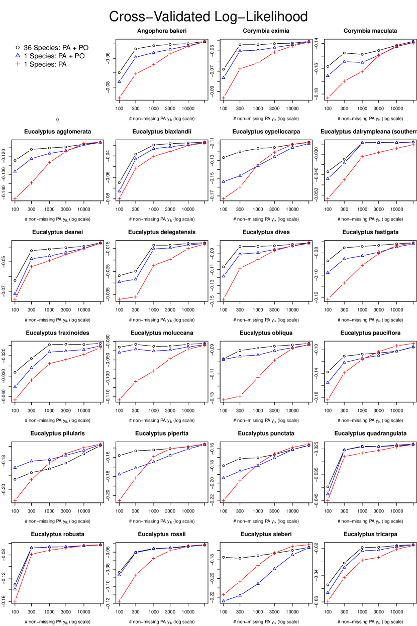
Figure 11: Cross-validation results for all species that were observed in at least 110 different presence-absence sites. Results vary for different species and different methods, but the method that pooled data across all 36 species had consistently superior performance.

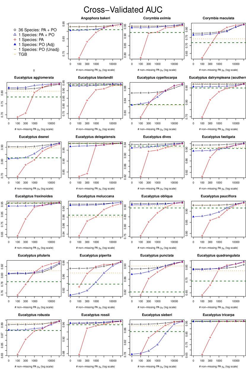
Figure 12: Cross-validation results for all species that were observed in at least 110 different presence-absence sites. Results vary for different species and different methods, but the method that pooled data across all 36 species had consistently superior performance.

See pages 1- of dataDescription.pdf

References

- Aarts et al. (2012) G. Aarts, J. Fieberg, and J. Matthiopoulos. Comparative interpretation of count, presence–absence and point methods for species distribution models. Methods in Ecology and Evolution, 3(1):177–187, 2012.
- Baddeley et al. (2010) A Baddeley, M Berman, NI Fisher, A Hardegen, RK Milne, D Schuhmacher, R Shah, and R Turner. Spatial logistic regression and change-of-support in poisson point processes. Electronic Journal of Statistics, 4:1151–1201, 2010.
- Chakraborty et al. (2011) Avishek Chakraborty, Alan E Gelfand, Adam M Wilson, Andrew M Latimer, and John A Silander. Point pattern modelling for degraded presence-only data over large regions. Journal of the Royal Statistical Society: Series C (Applied Statistics), 60(5):757–776, 2011.
- Cressie (1993) N.A.C. Cressie. Statistics for Spatial Data, revised edition, volume 928. Wiley, New York, 1993.
- Dorazio (2012) Robert M Dorazio. Predicting the geographic distribution of a species from presence-only data subject to detection errors. Biometrics, 68(4):1303–1312, 2012.
- Dudık et al. (2005) Miroslav Dudık, Robert E Schapire, and Steven J Phillips. Correcting sample selection bias in maximum entropy density estimation. Advances in neural information processing systems, 17:323–330, 2005.
- Efron and Tibshirani (1993) Bradley Efron and Robert Tibshirani. An introduction to the bootstrap, volume 57. CRC press, 1993.
- Elith et al. (2011) J. Elith, S.J. Phillips, T. Hastie, M. Dudík, Y.E. Chee, and C.J. Yates. A statistical explanation of maxent for ecologists. Diversity and Distributions, 2011.
- Fithian and Hastie (2013) William Fithian and Trevor Hastie. Finite-sample equivalence in statistical models for presence-only data. The Annals of Applied Statistics, 7(4):1917–1939, 2013.
- Gaetan and Guyon (2009) C. Gaetan and X. Guyon. Spatial statistics and modeling. Springer Verlag, 2009.
- Giraud et al. (2014) Christophe Giraud, Clément Calenge, and Romain Julliard. Capitalising on opportunistic data for monitoring biodiversity. arXiv preprint arXiv:1407.2432, 2014.
- Graham et al. (2008) Catherine H Graham, Jane Elith, Robert J Hijmans, Antoine Guisan, A Townsend Peterson, and Bette A Loiselle. The influence of spatial errors in species occurrence data used in distribution models. Journal of Applied Ecology, 45(1):239–247, 2008.
- Guan and Loh (2007) Yongtao Guan and Ji Meng Loh. A thinned block bootstrap variance estimation procedure for inhomogeneous spatial point patterns. Journal of the American Statistical Association, 102(480):1377–1386, 2007.
- Hall et al. (1995) Peter Hall, Joel L Horowitz, and Bing-Yi Jing. On blocking rules for the bootstrap with dependent data. Biometrika, 82(3):561–574, 1995.
- Hastie et al. (2009) T. Hastie, R. Tibshirani, and J. Friedman. The elements of statistical learning. Springer Series in Statistics, 2009.
- Hastie and Fithian (2013) Trevor Hastie and Will Fithian. Inference from presence-only data; the ongoing controversy. Ecography, 36(8):864–867, 2013.
- Hefley et al. (2013a) Trevor J Hefley, David M Baasch, Andrew J Tyre, and Erin E Blankenship. Correction of location errors for presence-only species distribution models. Methods in Ecology and Evolution, 2013a.
- Hefley et al. (2013b) Trevor J Hefley, Andrew J Tyre, David M Baasch, and Erin E Blankenship. Nondetection sampling bias in marked presence-only data. Ecology and Evolution, 2013b.
- Lawson et al. (2014) Callum R Lawson, Jenny A Hodgson, Robert J Wilson, and Shane A Richards. Prevalence, thresholds and the performance of presence–absence models. Methods in Ecology and Evolution, 5(1):54–64, 2014.
- Lehmann and Casella (1998) Erich Leo Lehmann and George Casella. Theory of point estimation, volume 31. Springer, 1998.
- Lele and Keim (2006) Subhash R Lele and Jonah L Keim. Weighted distributions and estimation of resource selection probability functions. Ecology, 87(12):3021–3028, 2006.
- Lele et al. (2012) Subhash R Lele, Monica Moreno, and Erin Bayne. Dealing with detection error in site occupancy surveys: what can we do with a single survey? Journal of Plant Ecology, 5(1):22–31, 2012.
- Lindenmayer et al. (2009) David B Lindenmayer, Alan Welsh, Christine Donnelly, Mason Crane, Damian Michael, Christopher Macgregor, Lachlan McBurney, Rebecca Montague-Drake, and Philip Gibbons. Are nest boxes a viable alternative source of cavities for hollow-dependent animals? long-term monitoring of nest box occupancy, pest use and attrition. Biological conservation, 142(1):33–42, 2009.
- McCullagh and Nelder (1989) P McCullagh and John A Nelder. Generalized Linear Models, volume 37. CRC Press, 1989.
- Nordman et al. (2007) Daniel J Nordman, Soumendra N Lahiri, and Brooke L Fridley. Optimal block size for variance estimation by a spatial block bootstrap method. Sankhyā: The Indian Journal of Statistics, pages 468–493, 2007.
- Pearce and Boyce (2006) Jennie L Pearce and Mark S Boyce. Modelling distribution and abundance with presence-only data. Journal of Applied Ecology, 43(3):405–412, 2006.
- Phillips et al. (2009) Steven J Phillips, Miroslav Dudík, Jane Elith, Catherine H Graham, Anthony Lehmann, John Leathwick, and Simon Ferrier. Sample selection bias and presence-only distribution models: implications for background and pseudo-absence data. Ecological Applications, 19(1):181–197, 2009.
- Renner and Warton (2013) Ian W Renner and David I Warton. Equivalence of maxent and poisson point process models for species distribution modeling in ecology. Biometrics, 2013.
- Renner et al. (2014) Ian W Renner, Adrian Baddeley, Jane Elith, William Fithian, Trevor Hastie, Steven Phillips, Gordana Popovic, and David I Warton. Point process models for presence-only analysis — a review. Methods in Ecology and Evolution, 2014.
- Royle and Dorazio (2008) J Andrew Royle and Robert M Dorazio. Hierarchical modeling and inference in ecology: the analysis of data from populations, metapopulations and communities. Academic Press, 2008.
- Royle and Nichols (2003) J Andrew Royle and James D Nichols. Estimating abundance from repeated presence-absence data or point counts. Ecology, 84(3):777–790, 2003.
- Royle et al. (2012) J Andrew Royle, Richard B Chandler, Charles Yackulic, and James D Nichols. Likelihood analysis of species occurrence probability from presence-only data for modelling species distributions. Methods in Ecology and Evolution, 3(3):545–554, 2012.
- Sólymos et al. (2012) Péter Sólymos, Subhash Lele, and Erin Bayne. Conditional likelihood approach for analyzing single visit abundance survey data in the presence of zero inflation and detection error. Environmetrics, 23(2):197–205, 2012.
- Ward et al. (2009) G. Ward, T. Hastie, S. Barry, J. Elith, and J.R. Leathwick. Presence-only data and the em algorithm. Biometrics, 65(2):554–563, 2009.
- Warton et al. (2013) David I Warton, Ian W Renner, and Daniel Ramp. Model-based control of observer bias for the analysis of presence-only data in ecology. PloS one, 8(11):e79168, 2013.
- Warton and Shepherd (2010) D.I. Warton and L.C. Shepherd. Poisson point process models solve the ”pseudo-absence problem” for presence-only data in ecology. The Annals of Applied Statistics, 4(3):1383–1402, 2010.
- Yee and Mitchell (1991) Thomas W Yee and Neil D Mitchell. Generalized additive models in plant ecology. Journal of vegetation science, 2(5):587–602, 1991.
- Zaniewski et al. (2002) A Elizabeth Zaniewski, Anthony Lehmann, and Jacob McC Overton. Predicting species spatial distributions using presence-only data: a case study of native new zealand ferns. Ecological modelling, 157(2):261–280, 2002.