Parametric Analytical Preconditioning and its Applications to the Reduced Collocation Methods

Abstract

In this paper, we extend the recently developed reduced collocation method [4] to the nonlinear case, and propose two analytical preconditioning strategies. One is parameter independent and easy to implement, the other one has the traditional affinity with respect to the parameters which allows for efficient implementation through an offline-online decomposition. Overall, the preconditioning improves the quality of the error estimation uniformly on the parameter domain, and speeds up the convergence of the reduced solution to the truth approximation.

Résumé On étend dans cette note la méthode de collocation réduite récemment introduite dans [4] au cas non linéaire et on propose deux stratégies de préconditionnement dont une est indépendante des paramètres et facile a mettre en oeuvre et l’autre possède la propriété classique de décomposition affine qui permet une mise en oeuvre rapide en-ligne/hors-ligne. Ces stratégies améliorent la qualité de l’approximation et la vitesse de convergence.

, , ,

Presented by Olivier Pironneau

Version française abrégée

La méthode de base réduite classique (RBM)[3, 7, 8, 9] pour l’approximation de la solution d’équations aux dérivées partielles (EDP) paramétrées du type $[\mathbb{L}(\mu)\,u_{\mu}](x)=f(x;\mu),\,\,x\in\Omega\,\,\,{\color[rgb]{0,0,0}\subset\mathbb{R}^{n}}$ repose sur la définition d’un espace de discrétisation ad’hoc, engendré par des solutions particulières de l’EDP en certain paramètres bien choisis. Ces solutions particulières doivent être préalablement approchées par une méthode traditionnelle spectrale ou d’éléments finis par exemple. Elle est principalement développée dans le cadre variationnel et permet la résolution en temps bien plus faible que des méthodes traditionnelles. Dans certain cadres, néanmoins, l’approche de collocation est préférable à l’approche variationnelle, en particulier lorsque la physique est complexe. La méthode de collocation réduite récemment introduite dans [4] permet de poser le problème de cette façon. Ainsi lorsque la méthode traditionnelle est de type spectrale collocation où, après avoir définit un opérateur discret $\mathbb{L}_{\mathcal{N}}(\mu)$, on cherche un polynôme $u^{\mathcal{N}}_{\mu}$ tel que $[\mathbb{L}_{\mathcal{N}}(\mu)\,u^{\mathcal{N}}_{\mu}](x_{j})=f(x_{j};\mu)$ est vérifié exactement sur un ensemble de ${\mathcal{N}}$ points de collocation $C^{\mathcal{N}}=\{x_{j}\}_{j=1}^{\mathcal{N}}$, l’approche de collocation réduite propose une approximation $u^{(N)}_{\mu^{*}}$: $u^{(N)}_{\mu^{*}}=\sum_{j=1}^{N}c_{j}(\mu^{*})u^{\mathcal{N}}_{\mu^{j}}$ vérifiant (1) soit au sens des moindre carré (LSRCM), puisqu’il y a plus de point $x_{k}$ que de coefficients $c_{j}$ (en effet $N<\!<{\mathcal{N}}$) soit seulement en certain points bien choisis $x\in C_{R}^{N}$ (ERCM).

Les méthodes de collocation sont connues pour être moins stables que les méthodes variationnelles. Pour rectifier cet inconvévient, nous proposons deux types de préconditionnement analytique, basés sur la définition d’un opérateur de prćonditionnement $P$ et sur une approximation de $P\mathbb{L}_{\mathcal{N}}(\mu)\,u^{\mathcal{N}}_{\mu}(x_{j})\simeq Pf(x_{j};\mu)$ dans les deux sens précédents. Les deux opérateurs de préconditionnement analytiques sont : une version indépendante du paramètre $P^{\mu^{c}}:=\mathbb{L}_{\mathcal{N}}(\mu^{c})^{-1}$, qui améliore l’approximation surtout au niveau de la valeur barycentrale $\mu^{c}$ et une version paramétrée qui, dans le cas où l’ensemble des paramètres est le carré $[0,1]^{2}$ repose sur une interpolation $Q_{1}$ entre les 4 valeurs de $\mathbb{L}_{\mathcal{N}}(\mu)^{-1}$ aux coins du domaine paramétrique: $P^{I}(\mu)=P_{00}(1-\mu^{1})(1-\mu^{2})+P_{01}(1-\mu^{1})\mu^{2}+P_{10}\mu^{1}(1-\mu^{2})+P_{11}\mu^{1}\mu^{2}$. Les illustrations numériques des performance de ces deux préconditionnement analytiques sont proposées dan les figures 2 et 3. La figure 2 illustre la comparaison des trois opérateurs analytiques de préconditionnement : sur la gauche sont tracés les indices d’effectivité de l’estimation de l’erreur sur le système avec ces opérateurs de préconditionnement. Sur la droite sont tracés la pire des convergences selon ces scénarii. La figure 3 illustre l’histoire de la convergence selon les opérateurs analytiques de préconditionnement pour l’approche des moindres carrés (à gauche) et l’approche empirique de collocation (à droite).

Enfin une extension de l’approche de collocation réduite empirique aux cas d’EDP non linéaire est aussi proposée et consiste naturellementt en la vérification de l’EDP non linéaire en des points de collocation choisis de façon empirique.

1 Introduction

The Reduced Basis Method (RBM)[3, 7, 8, 9] has been developed to numerically solve PDEs in scenarios that require a large number of numerical solutions to a parametrized PDE, and in which we are ready to expend significant computational time to pre-compute data that can be later used to compute accurate solutions in real-time. The RBM splits the solution procedure into two parts: an offline part where a greedy algorithm is utilized to judiciously select $N$ parameter values for pre-computation; and an online part where the solution for many new parameter is efficiently approximated by a Galerkin projection onto the low-dimensional space spanned by these $N$ pre-computed solutions.

While Galerkin methods (that are mostly used for RBM) are derived by requiring that the projection of the residual onto a prescribed space is zero, collocation methods require the residual to be zero at some pre-determined collocation points. They are attractive for their ease of implementation, particularly for time-dependent nonlinear problems [5, 10]. In [4], two of the authors developed the so-called Reduced Collocation Method (RCM). It adopts the RBM idea for collocation methods providing a strategy to practitioners who prefer a collocation, rather than Galerkin, approach. Our current implementation of this new method uses collocation for both the truth solver and the online reduced solver, but the offline part could be based on a variational approach as well. Furthermore, one of the two approaches in [4], the empirical reduced collocation method (ERCM) allows to eliminate a potentially costly online procedure that is needed for non-affine problems with a Galerkin approach. The method’s efficiency matches (or, for non-affine problems, exceeds) that of the traditional RBM in the Galerkin framework.

However, collocation methods may suffer from bad conditioning. In this paper, we propose and test two analytical preconditioning strategies to address this issue in the parametric setting of RCM. One strategy is parameter independent, which is advantageous for ease of implementation. The other one is parameter dependent, but has the traditional affinity with respect to the parameters which allows extremely efficient implementation through an offline-online decomposition. Overall, we show that the preconditioning uniformly improves the quality of the approximation, and speeds up the convergence of the solution process without adversely impacting the efficiency of the method in any significant way. While the focus and novelty of this paper is primarily the design of the analytical preconditioners, we also describe the extension of the RCM to the nonlinear case. In Section 2, we briefly review RCM and describe our analytical preconditioners. Numerical results are provided in Section 3.

2 The Algorithms

We begin with a linear parametrized PDE depending on a parameter $\mu\in{\mathcal{D}}\subset\mathbb{R}^{d}$, written in a strong form as $[\mathbb{L}(\mu)\,u_{\mu}](x)=f(x;\mu),\,\,x\in\Omega\,\,\,{\color[rgb]{0,0,0}\subset\mathbb{R}^{n}}$ with appropriate boundary conditions. We approximate the solution to this equation using a collocation approach: for any $\mu\in{\mathcal{D}}$, we define a discrete differentiation operator $\mathbb{L}_{\mathcal{N}}(\mu)$, and a discrete (polynomial) solution $u^{\mathcal{N}}_{\mu}$ such that $[\mathbb{L}_{\mathcal{N}}(\mu)\,u^{\mathcal{N}}_{\mu}](x_{j})=f(x_{j};\mu)$ on a given set of collocation points $C^{\mathcal{N}}=\{x_{j}\}_{j=1}^{\mathcal{N}}$, usually taken as a tensor product of ${\mathcal{N}}_{x}$ collocation points for each dimension that is allowed by rectangular domains. We assume that the resulting approximate solution $u^{\mathcal{N}}_{\mu}$ is highly accurate and refer to it as the “truth approximation”.

2.1 Online algorithms

For completeness, we briefly outline the RCM [4]. The idea is that when the solution for any parameter value $\mu^{*}\in{\mathcal{D}}$ is needed, instead of solving for the costly truth approximation $u^{\mathcal{N}}_{\mu^{*}}$, we somehow combine $N$ pre-computed truth approximations $u^{\mathcal{N}}_{\mu^{1}},\,\dots,\,u^{\mathcal{N}}_{\mu^{N}}$ to produce a surrogate solution $u^{(N)}_{\mu^{*}}$: $u^{(N)}_{\mu^{*}}=\sum_{j=1}^{N}c_{j}(\mu^{*})u^{\mathcal{N}}_{\mu^{j}}.$ The key feature of the algorithm is the requirement that the surrogate solution $u^{(N)}_{\mu^{*}}$ will satisfy the discretized differential equation in some sense $\mathbb{L}_{\mathcal{N}}(\mu^{*})u^{(N)}_{\mu^{*}}\approx f({\color[rgb]{0,0,0}\cdot};\mu^{*}).$ Exploiting the linearity of the operator, we observe that the system of equations we wish to solve is : find $\vec{c}(\mu^{*})$ such that

$$\vec{c}(\mu^{*})=(c_{1}(\mu^{*}),c_{2}(\mu^{*}),\dots,c_{N}(\mu^{*}))^{T},\quad\sum_{j=1}^{N}c_{j}(\mu^{*})[\mathbb{L}_{\mathcal{N}}(\mu^{*})u^{\mathcal{N}}_{\mu^{j}}](x_{k})\approx f(x_{k};\mu^{*})\;\;\;\;.$$ (1)

Satisfying the above equation exactly for $k=1,...,{\mathcal{N}}$ is usually an overdetermined system since we have only $N$ unknowns, but ${\mathcal{N}}>>N$ equations.

Least squares approach. When faced with an overdetermined system, we can determine the coefficients by satisfying the equation (1) in a least squares sense: we define, for any $\mu^{*}$, an ${\mathcal{N}}\times N$ matrix $\mathbb{A}_{N}(\mu^{*})$ with $j^{\rm th}$ column $\mathbb{L}_{\mathcal{N}}(\mu^{*})\,u_{\mu^{j}}^{\mathcal{N}}$, and vector of length ${\mathcal{N}}$, ${\mathbf{f}}^{\mathcal{N}}_{j}(\mu^{*})=f(x_{j};\mu^{*})\;\;x_{j}\in C^{\mathcal{N}},$ and solve the least squares problem $\mathbb{A}_{N}^{T}(\mu^{*})\,\mathbb{A}_{N}(\mu^{*})\,\vec{c}(\mu^{*})=\mathbb{A}_{N}^{T}(\mu^{*})\,{\mathbf{f}}^{\mathcal{N}}(\mu^{*})$to obtain $\vec{c}(\mu^{*})$.

Reduced Collocation approach. Our second approach is more natural from the collocation point-of-view. We determine the coefficients $\mathbf{c}(\mu^{*})$ by enforcing (1) at a reduced set of collocation points $C_{R}^{N}$. In other words, we solve $\sum_{j=1}^{N}c_{j}(\mu^{*})[\mathbb{L}_{\mathcal{N}}(\mu^{*})u^{\mathcal{N}}_{\mu^{j}}](x)=f(x;\mu^{*})$, for $x\in C_{R}^{N}$, which can also be written as $\mathbb{{\color[rgb]{0,0,0}I}}_{\mathcal{N}}^{N}\mathbb{A}_{N}(\mu^{*})\,\vec{c}(\mu^{*})=\mathbb{{\color[rgb]{0,0,0}I}}_{\mathcal{N}}^{N}{\mathbf{f}}^{\mathcal{N}}$, where $\mathbb{{\color[rgb]{0,0,0}I}}_{\mathcal{N}}^{N}$ is a $N\times{\mathcal{N}}$ matrix, that extracts the $N$ values of a ${\mathcal{N}}-$vector associated to the indices of the reduced set of collocation points. Later we will demonstrate how this set of points can be determined, together with the choice of basis functions, through the greedy algorithm.

2.2 Offline-online decomposition

The size of the matrix we need for solving $\vec{c}(\mu^{*})$ for each new $\mu^{*}$ is $N\times N$, but its assembly is not obviously independent of ${\mathcal{N}}$. For that purpose, we need the affine assumption on the operator as in the Galerkin framework. Thus, the overall online component is independent of ${\mathcal{N}}$ after a preparation stage where all the parameter independent quantities are precomputed [4]. We remark that there are remedies available when the parameter-dependence is not affine [2].

2.3 Analytical Preconditioning

Collocation methods are frequently ill-conditioned. The situation is exacerbated when we form the normal equation in the Least Squares approach. In this section, we propose two analytical preconditioning techniques. One is parameter-independent and the other is parameter-dependent. Both will provide an operator $P$ such that the discretization is based on the minimization of $P\mathbb{L}_{\mathcal{N}}(\mu)\,u^{\mathcal{N}}_{\mu}(x_{j})-Pf(x_{j};\mu)$ and the reduced problem in, e.g. the second approach becomes $\sum_{j=1}^{N}c_{j}(\mu^{*})\mathbb{{\color[rgb]{0,0,0}I}}_{\mathcal{N}}^{N}\left(P\mathbb{L}_{\mathcal{N}}(\mu^{*})u^{\mathcal{N}}_{\mu^{j}}\right)=\mathbb{I}_{\mathcal{N}}^{N}(Pf).$

Parameter-independent approach: We propose using $P^{\mu^{c}}:=\mathbb{L}_{\mathcal{N}}(\mu^{c})^{-1}$ as a preconditioning operator. Here $\mu^{c}$ is the center of the parameter domain ${\mathcal{D}}$. We remark that this preconditioner is in general, ideal for $\mu=\mu^{c}$ (making condition number exactly $1$). Moreover, it is affordable in the parametric setting since we can perform the ${\mathcal{N}}-$dependent operations for the offline preconditioning once for all.

Parameter-dependent approach: $P^{\mu^{c}}$ works well. However, it is more effective when $\mu$ is close to $\mu^{c}$. To have a preconditioning operator working well uniformly on the parameter domain, we need a parameter-dependent one. In addition, for the preconditioning to be meaningful in our parametric setting, a key requirement is that it satisfies an affine property similar to those for the operator $\mathbb{L}_{N}(\mu)$.

Assuming our ($d-$dimensional) parameter domain is rectangular, we form $2^{d}$ operators at the vertices of the domain: $\mathbb{L}_{\mathcal{N}}(\mu^{V_{i}})$ for $i=1,\dots,2^{d}$, find their inverses $P_{V_{i}}=\left(\mathbb{L}_{\mathcal{N}}(\mu^{V_{i}})\right)^{-1}$, and define the preconditioning operator through interpolation. In the case $d=2$ (we assume $\mu=(\mu^{1},\mu^{2})\in[0,1]^{2}$ without loss of generality), this is a $Q_{1}$ interpolation defined as below: $P^{I}(\mu)=P_{00}(1-\mu^{1})(1-\mu^{2})+P_{01}(1-\mu^{1})\mu^{2}+P_{10}\mu^{1}(1-\mu^{2})+P_{11}\mu^{1}\mu^{2},$ where $P_{ij}$ is $P_{V}$ with $V$ being the $(i,j)-$corner.

2.4 Offline algorithms

In this section we describe the two greedy algorithms for the least squares and the reduced collocation approaches for choosing the reduced basis set $\{u_{\mu^{1}}^{\mathcal{N}},\dots,u_{\mu^{N}}^{\mathcal{N}}\}$. We assume that given $\{u_{\mu^{1}}^{\mathcal{N}},\dots,u_{\mu^{i}}^{\mathcal{N}}\}$ we can compute an upper bound $\Delta_{i}(\mu)$ for the error of the reduced solution $u_{\mu}^{(i)}$ for any parameter $\mu$ [4].

Algorithm 1 Least Squares Reduced Collocation Method (LSRCM): Offline Procedure

  1. Discretize the parameter domain ${\mathcal{D}}$ by $\Xi$, and denote the center of ${\mathcal{D}}$ by $\mu^{c}$.

  2. Randomly select $\mu^{1}$, solve $\mathbb{L}_{\mathcal{N}}(\mu^{1})\,u^{\mathcal{N}}_{\mu^{1}}(x)=f(x;\mu^{1})$ for $x\in C^{\mathcal{N}}$ and let $\xi_{1}^{\mathcal{N}}=u^{\mathcal{N}}_{\mu^{1}}$.

  3. For $i=2,\dots,N$ do

• For all $\mu\in\Xi$, form $\mathbb{A}_{i-1}(\mu)=\left(\mathbb{L}_{\mathcal{N}}(\mu)\,\xi_{1}^{\mathcal{N}},\mathbb{L}_{\mathcal{N}}(\mu)\,\xi_{2}^{\mathcal{N}},\,\dots,\,\mathbb{L}_{\mathcal{N}}(\mu)\,\xi_{{i-1}}^{\mathcal{N}}\right)$.

• For all $\mu\in\Xi$, solve $\mathbb{A}_{i-1}(\mu)^{T}\,\mathbb{A}_{i-1}(\mu)\,\vec{c}=\mathbb{A}_{i-1}^{T}(\mu)\,{\mathbf{f}}^{\mathcal{N}}$ to obtain $u^{(i-1)}_{\mu}=\sum_{j=1}^{i-1}c_{j}\xi^{\mathcal{N}}_{j}$ and $\Delta_{i-1}(\mu)$.

• Set $\mu^{i}=argmax_{\mu}\,\,\Delta_{i-1}(\mu)$, and solve $\mathbb{L}_{\mathcal{N}}(\mu^{i})\,u^{\mathcal{N}}_{\mu^{i}}(x)=f(x;\mu^{i})$ for $x\in C^{\mathcal{N}}$.

• Apply a modified Gram-Schmidt transformation, with inner product defined by

  $(u,v)\equiv\left(\mathbb{L}_{\mathcal{N}}(\mu^{c})u,\mathbb{L}_{\mathcal{N}}(\mu^{c})v\right)_{L^{2}(\Omega)}$, on $\left\{\xi^{\mathcal{N}}_{1},\xi^{\mathcal{N}}_{2},\dots,\xi^{\mathcal{N}}_{i-1},u^{\mathcal{N}}_{\mu^{i}}\right\}$ to obtain $\left\{\xi_{1}^{\mathcal{N}},\xi_{2}^{\mathcal{N}},\dots,\xi_{i}^{\mathcal{N}}\right\}$.

Algorithm 2 Empirical Reduced Collocation Method (ERCM): Offline Procedure

  1. Randomly select $\mu^{1}$, solve $\mathbb{L}_{\mathcal{N}}(\mu^{1})\,u^{\mathcal{N}}_{\mu^{1}}(x)=f(x;\mu^{1})$, let $x^{1}=argmax_{x\in X}\,\,\left|u^{\mathcal{N}}_{\mu^{1}}(x)\right|,\quad\xi^{\mathcal{N}}_{1}=\frac{u^{\mathcal{N}}_{\mu^{1}}}{u^{\mathcal{N}}_{\mu^{1}}(x^{1})}$.

  2. For $i=2,\dots,N$ do

• Let $C_{R}^{i-1}=\left\{x^{1},\dots,x^{i-1}\right\}$.

• For all $\mu\in\Xi$, solve  $\sum_{j=1}^{i-1}c_{j}\mathbb{I}_{\mathcal{N}}^{N}\left(\mathbb{L}_{\mathcal{N}}(\mu)u^{\mathcal{N}}_{\mu^{j}}\right)=f(x;\mu)\,\,{\rm for}\,\,x\in C_{R}^{i-1}$ to obtain $u^{(i-1)}_{\mu}=\sum_{j=1}^{i-1}c_{j}u^{\mathcal{N}}_{\mu^{j}}$.

• Set $\mu^{i}=argmax_{\mu\in\Xi}\,\,\Delta_{i-1}(\mu)$ and solve $\mathbb{L}_{\mathcal{N}}(\mu^{i})\,u^{\mathcal{N}}_{\mu^{i}}(x)=f(x;\mu^{i})$.

• Find $\alpha_{1},\dots,\alpha_{i-1}$ such that, if we define $\xi^{\mathcal{N}}_{i}=u^{\mathcal{N}}_{\mu^{i}}-\sum_{j=1}^{i-1}\alpha_{j}\,\xi^{\mathcal{N}}_{j}$, we have $\xi^{\mathcal{N}}_{i}(x^{j})=0$ for $j=1,\dots,i-1$.

• Set $x^{i}=argmax_{x}\,\,\left|\xi^{\mathcal{N}}_{i}\right|$ and $\xi^{\mathcal{N}}_{i}=\frac{\xi^{\mathcal{N}}_{i}}{\xi^{\mathcal{N}}_{i}(x^{i})}$.

• Apply modified Gram-Schmidt transformation on $\left\{\xi_{1}^{\mathcal{N}},\dots,\xi_{i}^{\mathcal{N}}\right\}$.

2.5 Extension to the nonlinear case

The ERCM approach is more economical than the EIM implementation of the variational RBM for linear problems having a large number of varying coefficients, such as the case when geometry is a parameter [6]. Here, we outline the procedure when we have a general nonlinear operator $\mathbb{G}(u;\mu)+\mathbb{L}(\mu)u$ where $\mathbb{G}(u;\mu)$ is nonlinear. The parameter dependence can be handled in the same way with possibly the Empirical Interpolation [2] needed, so it suffices to assume $\mathbb{G}(u;\mu)\equiv\mathbb{G}(u)$. In the following, we present our approach through the example of the viscous Burgers’ equation $uu_{x}-\mu u_{xx}=f_{\mu}$; The formal extension to multi-dimension vector equations is straightforward. In the case of Burgers’ equation, the discretized system for any parameter $\mu^{j}$ becomes $\mathbf{u}\odot\mathbf{D}\mathbf{u}-\mu^{j}\mathbf{D}_{2}\mathbf{u}=f_{\mu^{j}},$ where $\mathbf{u}$ is the ${\mathcal{N}}\times 1$ vector containing the point values of $u$ on the Chebyshev grid, $\odot$ is the well-known Hadamard product for vectors that denotes element wise multiplication, and $\mathbf{D}$ and $\mathbf{D}_{2}$ are the ${\mathcal{N}}\times{\mathcal{N}}$ first and second order differentiation matrices, respectively. We assume that we are given $N$ solutions $u_{\mu^{j}}^{\mathcal{N}}$ and we define $u^{(N)}_{\mu^{*}}=\sum_{j=1}^{N}c_{j}(\mu^{*})u_{\mu^{j}}^{\mathcal{N}}$. We find the values of the unknown coefficients $c_{j}$ by satisfying a nonlinear equation of the form $G(\mathbf{c})-\mu^{*}\mathbf{L}\mathbf{c}=f_{\mu^{*}}$. Here, $\mathbf{c}$ is the column vector of coefficients $c_{j}$ of length $N$, $\mathbf{L}$ is an $N\times N$ matrix, and $G:\mathbb{R}^{N\times 1}\rightarrow\mathbb{R}^{N\times 1}$ is a nonlinear function. These solutions are then solved by some iterative fixed-point like method. For the ERCM case, $\mathbf{L}$ and $G$ come from the discrete solution satisfying $\mathbf{u}\odot\mathbf{D}\mathbf{u}-\mu^{*}\mathbf{D}_{2}\mathbf{u}=f_{\mu^{*}}$ at a reduced set of collocation points $C_{R}^{N}$.

3 Numerical Results

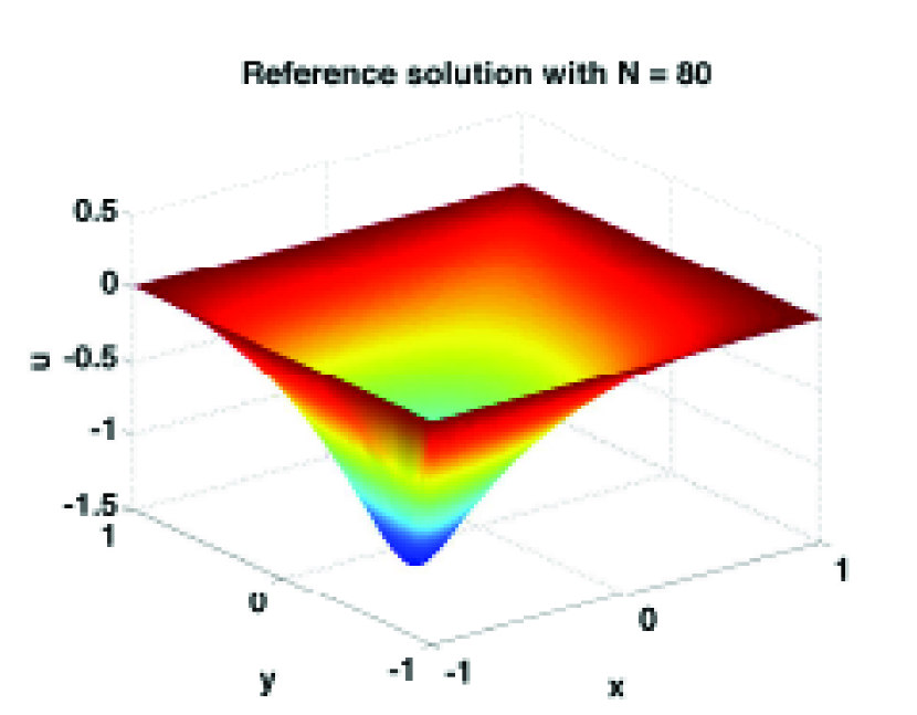
Figure 1: The truth approximationfor $\mu_{1}=1$ and $\mu_{2}=0.5$ computed on a $81\times 81$ Chebyshev grid.

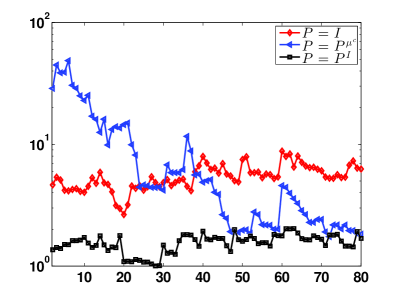
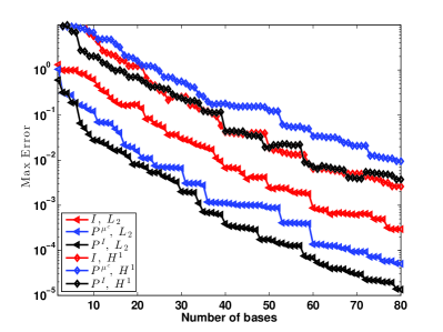
Figure 2: Comparison of the three analytical preconditioning operators: On the left is the plot for the effectivity indices for the error estimate on the system with these preconditioning operators. On the right are the worst case scenario convergence plots.

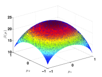
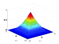
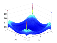
Figure 3: From left to right: the non-preconditioned inf-sup number ($P=I$), Parameter-independent preconditioning ($P=P^{\mu^{c}}$), and $Q_{1}$-interpolating parametric preconditioning ($P=P^{I}(\mu)$).

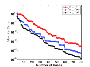
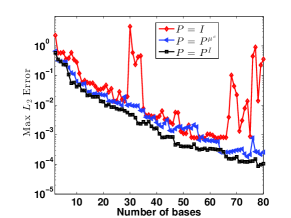
Figure 4: Comparison of history of convergence when different analytical preconditioning operators is used for the least squares approach (left) and empirical collocation approach (right). Maximum is taken among $L_{2}$ errors between truth approximation and reduced basis solution for $1,057$ randomly selected parameter values.

In this section, we demonstrate the accuracy and efficiency of the proposed methods on a 2D diffusion-type problem with zero Dirichlet boundary condition [4]: $(1+\mu_{1}x)u_{xx}+(1+\mu_{2}y)u_{yy}=e^{4xy}\,\,\mbox{ on }\Omega=[-1,1]\times[-1,1].$ Our truth approximations are generated by a spectral Chebyshev collocation method [10, 5]. For $C^{\mathcal{N}}$, we use the Chebyshev grid based on ${\mathcal{N}}_{x}$ points in each direction with ${\mathcal{N}}_{x}^{2}={\mathcal{N}}$. We consider the parameter domain ${\mathcal{D}}$ for $(\mu_{1},\mu_{2})$ to be $[-0.99,0.99]^{2}$. For $\Xi$, they are discretized uniformly by a $64\times 64$ Cartesian grid. One sample solution for this problem is plotted in Figure 2.

In Figure 2 (Left), we show that while the non-parametric preconditioning $P^{\mu^{c}}$ give non-uniform improvement, the parametric preconditioning $P^{I}(\mu)$ improves effectivity indices by one order of magnitude. Figure 2 (Right) shows that the $P^{\mu^{c}}$ preconditioning operator improves the $L_{2}$ norm of the error but worsens the $H^{1}$ norm. In comparison, $P^{I}(\mu)$ improves the error in $L^{2}$ norm without significantly degrading (in some cases improving) the error in $H^{1}$ norm. Finally, we plot the stability constant of these preconditioned operators as a function of the parameter in Figure 3. We clearly see that $P^{I}(\mu)$ is most efficient in terms of enforcing the parametric stability number uniformly close to $1$. We also tested diagonal preconditioning $P^{I}_{D}(\mu)$ (not reported here) by using the same interpolating procedure as $P^{I}(\mu)$ and replacing the inverses of the full operators by the inverses of the diagonals. Clearly $P^{I}_{D}(\mu)$ is cheaper to compute than the other preconditioners, but its performance is significantly worse than $P^{I}(\mu)$ and even worse than $P^{\mu^{c}}$.

For the preconditioned RCM, we can see, from Figures 4 that the error for the least squares approach is around one order of magnitude better in the worst case scenario. For the empirical reduced collocation approach, the error is smaller and, more importantly, converges much more stably.

4 Concluding Remarks

We propose and test two analytical preconditioning strategies in the context of reduced collocation method. The parameter dependent one is shown to be capable of offline-online decomposition, improving both the quality of error estimation uniformly on the parameter domain, and enabling the preconditioned reduced collocation method to converge much faster and more stably than the non-preconditioned version.

References

- [1]
- [2] M. Barrault, N. C. Nguyen, Y. Maday, and A. T. Patera. An “empirical interpolation” method: Application to efficient reduced-basis discretization of partial differential equations. C. R. Acad. Sci. Paris, Série I, 339:667–672, 2004.
- [3] A. Barrett and G. Reddien. On the reduced basis method. Z. Angew. Math. Mech., 75(7):543–549, 1995.
- [4] Y. Chen and S. Gottlieb. Reduced collocation methods: Reduced basis methods in the collocation framework. J. Sci. Comput., 55(3):718–737, 2013.
- [5] J. S. Hesthaven, S. Gottlieb, and D. Gottlieb. Spectral methods for time-dependent problems, volume 21 of Cambridge Monographs on Applied and Computational Mathematics. Cambridge University Press, Cambridge, 2007.
- [6] Y. Chen and S. Gottlieb. Reduced collocation methods: Reduced basis methods in the collocation framework. J. Sci. Comput., 55(3):718–737, 2013.
- [7] A. K. Noor and J. M. Peters. Reduced basis technique for nonlinear analysis of structures. AIAA Journal, 18(4):455–462, April 1980.
- [8] J. S. Peterson. The reduced basis method for incompressible viscous flow calculations. SIAM Journal on Scientific and Statistical Computing, 10(4):777–786, 1989.
- [9] C. Prud’homme, D. Rovas, K. Veroy, Y. Maday, A. T. Patera, and G. Turinici. Reliable real-time solution of parametrized partial differential equations: Reduced-basis output bound methods. Journal of Fluids Engineering, 124(1):70–80, March 2002.
- [10] L. N. Trefethen. Spectral methods in MATLAB, volume 10 of Software, Environments, and Tools. Society for Industrial and Applied Mathematics (SIAM), Philadelphia, PA, 2000.