Open Clusters in the Kepler Field, II. NGC 6866

Abstract

We have developed a maximum-likelihood procedure to fit theoretical isochrones to the observed cluster color-magnitude diagrams of NGC 6866, an open cluster in the Kepler Spacecraft field of view. The Markov-Chain Monte Carlo algorithm permits exploration of the entire parameter space of a set of isochrones to find both the best solution and the statistical uncertainties. For clusters in the age range of NGC 6866, with few if any red giant members, a purely photometric determination of the cluster properties is not well-constrained. Nevertheless, based on our UBVRI photometry alone, we have derived the distance, reddening, age and metallicity of the cluster and established estimates for the binary nature and membership probability of individual stars. We derive the following values for the cluster properties: $(m-M)_{V}=10.98\pm 0.24$, $E(B-V)=0.16\pm 0.04$ (so the distance = 1250 pc), age $=705\pm 170$ Myr and $Z=0.014\pm 0.005$.

1 Introduction

The four open clusters located in NASA’s Kepler spacecraft field of view (NGC 6866, NGC 6811, NGC 6819 and NGC 6791), which range in age from less than 1 Gyr to more than 8 Gyr, are ideal targets for a variety of astrophysical investigations. The two older clusters, NGC 6819 and NGC 6791 have been thoroughly studied (see, e.g., Corsaro et al., 2012; Sandquist et al., 2013; Yang et al., 2013, for recent Kepler-related papers), but the other two are less well-known. We recently completed an analysis of NGC 6811 (Janes et al., 2013, hereafter Paper I) and we report here on NGC 6866.

Recent publications on NGC 6866 include Frolov et al. (2010), who did a proper motion and CCD photometric study of the cluster; photometric studies by Molenda-Żakowicz et al. (2009) and Joshi et al. (2012); and an investigation by Balona et al. (2013) of rotations and pulsations of stars in the cluster using Kepler data. Frolov et al. found 423 likely cluster members and estimated the age of the cluster at 560 Myr. Joshi et al. derived $E(B-V)=0.10$ mag., an age of 630 Myr and a distance of 1.47 kpc. From an analysis of 2MASS JHK photometry, Güņes et al. (2012) derived an age 0.8$\pm$0.1 Gyr, E(B-V) = 0.19$\pm$0.06 and $(m-M)_{\circ}=11.08\pm 0.11$. Molenda-Żakowicz et al. and Joshi et al. both found several variable stars in the cluster. In a survey of a number of clusters, Frinchaboy & Majewski (2008) derived a radial velocity of 12.18 $\pm$ 1.14 km s^-1 and proper motions $\mu_{\alpha}cos\delta=-5.52\pm 1.17$ mas yr^-1 and $\mu_{\delta}=-7.97\pm 1.09$ mas yr^-1 for the cluster.

The traditional approach to deriving the properties of star clusters from broad-band photometry is to “fit” theoretical stellar isochrones to the observed color-magnitude diagram (CMD). But an isochrone is simply the locus of possible stars over a range of masses at fixed age in the CMD (see Figure 1a). So at a given time, in a cluster with a finite number of stars, it is unlikely that any stars will actually be found along some sections of an isochrone.

We have chosen instead to find the maximum-likelihood probability that the observed cluster stars embedded in a background population of field stars (Figure 2a) could be drawn from a theoretical CMD, created by choosing a sample of stars from the models with a range of masses, as in Figure 1b.

Figure 1: (a) A typical isochrone (Bressan et al., 2012) with age = 700 Myr and Z = 0.014 (see Table 3), (b) A theoretical CMD consisting of 100 stars selected at regular mass intervals from the same isochrone. We use the theoretical CMD for our analysis rather than the isochrone.

By posing the problem in this way, we can take a modern Bayesian approach to derive not only the cluster parameters, but also their uncertainties.

In §2 we describe the photometry; §3 is a discussion of the structural properties of the cluster; The Bayesian analysis is the topic of §4; §5 is a discussion of our results; and §6 summarizes our conclusions.

2 Photometric Program

We acquired CCD images of the cluster and standard stars on four nights (see Table 1), with the 1.2-meter Hall and 1.8-meter Perkins telescopes at Lowell Observatory. Since we did all of our NGC 6866 observing on nights when we also observed NGC 6811, the details of the observing and photometric reductions are given in Paper I. The following is a summary of the observational program.

Table 1: Observing Record

Date	2009 Sept 21	2009 Sept 25	2010 Sept 17	2010 Sept 18
Telescope	Perkins 1.8m	Hall 1.2m	Hall 1.2m	Hall 1.2m
Detector	Fairchild CCD	SITe CCD	e2v CCD	e2v CCD
Filters	B,V,R,I	B,V,I	U,B,V	U,B,V
No. of Stds.	93, 101, 96, 96	42, 34, 33	150, 129, 137	181, 188, 208
Field Size	13.3′ $\times$ 13.3′	37.9′ $\times$ 37.9′	42.8′ $\times$ 42.8′	42.8′ $\times$ 42.8′

Conditions were photometric on all four nights, and we imaged extensive sequences of Landolt standard stars (Landolt, 2009) over a wide range of airmass on each night, as noted in Table 1. We used IRAF bias subtraction and flat fielding functions for our initial image processing. We used the SPS program (Janes & Heasley, 1993) for PSF-fitting photometry and we transformed the photometry to the UBVRI colors as described in Paper I. The calculated uncertainties in the transformation coefficients are all less than 0.01 mag. The standard deviations of the nightly B and V values from the four-night means and the average differences between the two nights each in U and I photometry are all within 0.01 magnitude.

To aid in merging the measurements from individual frames, we used stars from the Kepler Input Catalog (Brown et al., 2011) to develop preliminary transformation coefficients to the equatorial system relative to the assumed cluster center at RA = 20^h 03^m 55.0^s, Dec = +44^∘ 09^′ 30.0^′′. We assumed that star images with transformed coordinates within 0.5 arcseconds of one another on different frames are the same star, except that we rejected stars if a single star image on one frame was within 0.5 arcseconds of two stars on another frame. We also rejected stars with fewer than 3 B or V measurents or fewer than 2 R or I measurements or if the calculated standard deviation of the V magnitude or B-V color index is 0.1 magnitude or greater.

The resulting catalog (Table 2) contains 7714 stars. Star numbers are in column 1, positions in arcseconds relative to the center ($X=\alpha cos(\delta)$ and $Y=\delta$) are in columns 2 and 3, the $V$ magnitudes and errors and $B-V$, $U-B$, $V-R$ and $V-I$ color indices and their errors are in the next 10 columns, and the final columns contain the numbers of measurements in each filter (in the order U, B, V, R, I). For the final catalog, we tied the preliminary merged star positions aproximately to the UCAC4 coordinate system (Zacharias et al., 2013).

Table 2: Photometric Catalog

Star	X	Y	V	B-V	U-B	V-R	V-I	NU	NB	NV	NR	NI
1	-1267.53	1151.81	14.642 $\pm$ 0.006	1.846 $\pm$ 0.014	$\cdots$	$\cdots$	$\cdots$	0	3	3	0	0
2	-1261.99	1088.49	16.410 $\pm$ 0.014	1.191 $\pm$ 0.026	$\cdots$	$\cdots$	$\cdots$	0	3	3	0	0
3	-1259.21	-132.86	16.202 $\pm$ 0.008	0.768 $\pm$ 0.016	$\cdots$	$\cdots$	$\cdots$	0	3	3	0	0
4	-1259.00	995.52	16.799 $\pm$ 0.016	0.885 $\pm$ 0.020	$\cdots$	$\cdots$	$\cdots$	0	3	3	0	0
5	-1256.87	648.49	12.586 $\pm$ 0.005	1.815 $\pm$ 0.009	$\cdots$	$\cdots$	$\cdots$	0	6	4	0	0

Note. — Table 2 is published in its entirety in the electronic edition of the Astronomical Journal. A portion is shown here for guidance regarding its form and content.

Figure 2a shows photometry for all stars in the catalog, covering a $42.8^{\prime}\times 42.8^{\prime}$ arcminute field, and Figure 2b is a CMD  derived from photometry of stars within a radius of 3 arcminutes from the cluster center.

Figure 2: (a) CMD for all stars in the catalog (field of view about $43\times 43$ arcminutes). The apparent discontinuity at magnitude 18.5 arises because the Hall 1.2-m frames cover a wider field, but are not as deep. (b) CMD for stars within a radius of 3 arcminutes from the cluster center only.

3 Cluster Structural Parameters

Using the data in Table 2, we derived the radial stellar density distribution about the cluster center. We calculated the areas of successive rings within which there are 75 stars between magnitudes 11 and 16. From that we found the stellar density in each ring, as shown in Figure 3. Because the cluster is relatively sparse and embedded in a rich star field, we chose a simple exponential function to model the radial stellar density profile:

$$\rho(r)=\rho_{cl}\thinspace exp\left({-r^{2}/\sigma_{r}^{2}}\right)+\rho_{f},$$ (1)

where, $\rho_{cl}$ refers to the peak of the radial stellar density distribution, $\rho_{f}$ is the background field stellar density. and the cluster core angular radius is $\sigma_{r}$.

Assuming the stellar density profile of Equation 1, the effective angular radius is $\sigma_{r}$ = 4.7 arcminutes and the peak cluster density is $\rho_{cl}$ = 1.65 stars per square arcminute on a field background of 0.63 stars per square arcminute. After subtracting the background, the integral of the exponential density function over all radii is

$$N_{cl}=\pi\rho_{cl}\thinspace\sigma_{r}^{2},$$ (2)

which gives a cluster population of 114 stars brighter than magnitude 16. This should be considered to be a lower limit to the cluster membership since there is likely to be an extended halo of stars photometrically undetectable against the background field population. Proper motions or radial velocities would be required to distinguish halo cluster stars from field stars; fortunately the goals of this project require only that a sufficiently large sample of high probability cluster stars be identified.

Figure 3: Radial density distribution of stars in NGC 6866. Each point represents the mean density of a ring containing 75 stars. The curve is an exponential with $\sigma_{r}=4.7$ arcminutes.

4 A Bayesian Analysis of NGC 6866

Bayes’ theorem states that

$$P({\bf m}|{\bf D})={P({\bf m})\mathcal{L}({\bf D}|{\bf m})\over P({\bf D})},$$ (3)

where $P({\bf m}|{\bf D})$ is the posterior probability distribution function (PDF) of the model parameters, ${\bf m}$, given the data, ${\bf D}$. $P({\bf m})$ is the prior PDF of the model parameters and $\mathcal{L}({\bf D}|{\bf m})$ is a likelihood function for the data, given a model. The denominator, $P({\bf D})$ is the integral of the numerator over all possible model parameters, and is ordinarily difficult to compute. However, it is effectively a normalizing constant, and the shape of the posterior PDF can be found without knowing $P({\bf D})$. A thorough discussion of Bayesian analysis can be found in Gregory (2005); for some astronomical applications, including deriving properties of star clusters, see Ford (2005), von Hippel et al. (2006) or De Gennaro et al. (2009). Our procedure is discussed in greater detail in Paper I. The following is a brief summary of our cluster analysis procedure.

Priors – The prior distribution, $P({\bf m})$, constitutes a model for the cluster. The model parameters include global properties of distance modulus, reddening and a theoretical CMD of some age and metallicity, as well as the membership probability and binary star status of individual stars. Because the global properties (distance modulus, reddening, age and metallicity) are chosen with equal probability within some range, their contribution to $P({\bf m})$ is effectively a constant and does not affect the shape of the posterior PDF. At each iteration, the model consisted of a theoretical CMD created from an isochrone of the specified age and metallicity by selecting a set of stars with random masses from the isochrone. The theoretical CMD was corrected for the particular values of reddening and distance selected at this iteration. We ran two sets of models, one using the “Yale-Yonsei” (YY) isochrones (Demarque et al., 2004) and the other using “Padova” isochrones (Bressan et al., 2012). The models were allowed to range over values of $0.000\leq E(B-V)\leq 0.30$; $10.0\leq(m-M)_{V}\leq 11.75;300\ Myr\leq$ age $\leq 1200\ Myr$; and $0.001\leq Z\leq 0.030$. All distance moduli calculated in this paper are observed, V-band moduli, uncorrected for interstellar extinction.

Cluster Membership – We computed the prior membership probability for individual stars, based on their distance relative to the cluster center using Equation 1. So the prior membership probability for star $i$ is a purely astrometric quantity,

$$a_{i}\propto exp(-r_{i}^{2}/\sigma_{r}^{2}).$$ (4)

At each iteration of the Markov chain, we randomly selected 125 stars from the entire field with prior membership probabilities given by Equation 4. That is to say, after randomly selecting a star from the catalog, we compared its prior membership probability as derived from Equation 1 with a randomly chosen number from zero to one. If the star’s membership probability exceeds that of the random number, it is added to the sample for that iteration. In this way, each star can be tested as a possible cluster member; stars which are more often present in successful trials have a higher posterior membership probability, as discussed in the following.

Binary Stars – The large fraction of binaries among open cluster stars makes it difficult to define the location of the actual single-star main sequence, particularly near the turnoff. However, the binary status of individual stars can be added as parameters in the Bayesian analysis. Each star is assigned a binary mass ratio, and the merged magnitude and colors of an equivalent binary in the theoretical CMD is calculated and compared to the observed star. For the initial iteration, the binary mass ratio for all stars was taken to be zero. At each subsequent iteration, the mass ratio is randomly perturbed from the previous value with a Gaussian probability (see the Hastings-Metropolis algorithm below).

Likelihood Function – For each observed star, $i$, we find the distance, $z_{i,j}$ in units of the measurement errors in the 5-dimensional CMD space (V, B-V, U-B, V-R, V-I) to each of the theoretical stars, $j$. The probability that $z_{i,j}$ is as small as it is by chance is the error function of $z_{i,j}$, $erf(z_{i,j})$. The probability that the observed star could be drawn from the CMD of theoretical stars is given by

$$p_{i}=1.0-\prod_{j}\Bigl{[}erf(z_{ij})\Bigr{]}.$$ (5)

So now from Equations 3 and 5, the operational Bayesian model is

$$P({\bf m}|{\bf D})=P({\bf m})\mathcal{L}({\bf D}|{\bf m})=P({\bf m})\prod_{i}p_{i},$$ (6)

which gives the probability that the observed sample of stars could be drawn from the theoretical sample.

Hastings-Metropolis Algorithm –- The key to efficient sampling of the PDF is to develop a “jump probability function,” $\alpha({\bf m_{t}}|{\bf m})$, to decide the transition from model ${\bf m}$ to a new trial model ${\bf m_{t}}$ so that ${\bf m_{t}}$ depends on the current parameters but not on any previous values. The trial model, ${\bf m_{t}}$, consists of random proposed jumps, $q({\bf m})$, from the current parameter values. The jump probability function can be written as

$$\alpha({\bf m}_{t}|{\bf m})=min\bigl{\{}{P({\bf m}_{t}|{\bf D})\thinspace\over P({\bf m}|{\bf D})}{q({\bf m}|{\bf m}_{t})\over q({\bf m}_{t}|{\bf m})},1\bigr{\}}.$$ (7)

If the jumps have a Gaussian distribution, the proposal distributions are symmetrical and in this case, $q({\bf m}|{\bf m}_{t})=q({\bf m}_{t}|{\bf m})$. A trial model is accepted as the next iteration when $\alpha$ exceeds a random number in the range 0 to 1; if the trial model is not accepted, another ${\bf m}_{t}$ is tested. Improved solutions are always selected, but in addition, the entire parameter space is eventually sampled. We ran two chains of 105000 trials; after throwing away the first 5000 trials in the “burn-in” period, we saved all trials satisfying the acceptance condition on the first try. See Paper I for more information.

Figure 4: Marginal distributions of cluster properties for the Yale chain: Number of samples vs: (a) reddening, E(B-V), (b) distance modulus, (c) age in Gyr and (d) metallicity, Z. In each figure, the solid curve represents a Gaussian fit to the distribution.

5 Discussion

The product of the above analysis is the posterior PDF, $P({\bf m}|{\bf D})$, a sequence of the parameter values for each successful trial. From the marginal distribution of each parameter (found by integrating $P({\bf m}|{\bf D})$ over all the other parameters), its mean and variance can be found. The marginal distributions are shown in Figure 4; although the scale of the distributions are defined only by the unknown parameter $P({\bf D})$, their means represent the maximum likelihood values of the parameters, and their standard deviations represent the parameter uncertainties. These are shown in Table 3.

Up to a constant, the prior PDF of an individual star is a single number, $a_{i}$, given by Equation 4. So now, the posterior PDF of star $i$ is just the product of $a_{i}$ and the individual likelihood parameter, $p_{i}$, given by Equation 5. In Figure 5 we included 125 stars with the largest values of the posterior membership probability.

For intermediate-age clusters like NGC 6866, with few if any giant stars, there is little information in the CMD to distinguish clusters by age or metallicity. This problem is intrinsic to isochrone fitting to clusters in this age range, independent of the details of the analysis technique. Furthermore, NGC 6866 is embedded in a rich field. As a consequence, although the procedure produces well-defined posterior PDF’s, the marginal distributions are rather broad –- i.e, the parameters are only moderately well constrained.

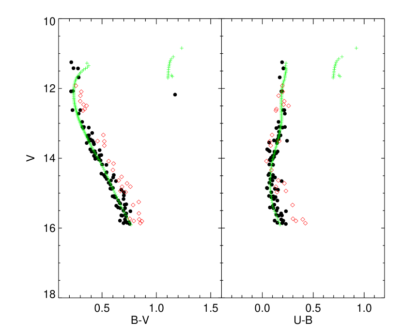
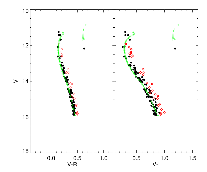
Figure 5: CMDs of the 125 stars in the cluster region with the largest posterior membership probabilities. Filled symbols: likely single stars; Open symbols: probable binary stars. Small crosses: theoretical CMD derived from the maximum-likelihood Padova isochrone. See the online edition for a color version of this figure.

The consequences of the indeterminancy between the effects of reddening and metallicity on photometry can be seen in Figure 6, a contour plot of the marginal distribution of the number of samples in the E(B-V) vs Z plane. Solutions with low reddening values tend to be correlated with those with high metallicity values. If one or the other were constrained by independent measures, the marginal distributions of the other parameters would be considerably sharper. There are indications of similar correlations between the other indices, but they are not as strong.

6 Conclusions

We have produced a catalog of high-quality Johnson/Cousins UBVRI photometry of stars in a large field around the cluster NGC 6866. Our photometry has been carefully transformed to the standard system as defined by the Landolt (2009) standard stars. Using a Bayesian analytical procedure, we derived the following values for the cluster properties: $(m-M)_{V}=10.98\pm 0.24$, $E(B-V)=0.16\pm 0.04$, age $=705\pm 170$ Myr and $Z=0.014\pm 0.005$ (see also Table 3). Assuming a canonical extinction-to-reddening ratio $R_{V}=A_{V}/E(B-V)=3.1$, the distance to the cluster is about 1250 parsecs.

Our results are in rough agreement with previous work on this cluster as discussed in the introduction (see also Balona et al., 2013, and references therein) As mentioned above, the lack of independent membership information, or, alternatively the cluster metallicity or reddening, limits the accuracy of photometric measurements of its age and distance. Furthermore, most of the previous results were based, directly or indirectly, on visual comparisons of observed color-magnitude diagrams with theoretical isochrones of solar composition only; for that reason, the quoted errors are likely to be highly optimistic, since they do not include the metallicity uncertainty. In particular, our analysis, as shown in Figures 4 and 6, do not support a metallicity as high as solar. Solar metallicity would require a reddening of essentially zero, unlikely in this direction in the galaxy.

Figure 6: Two-dimensional marginal distribution of the numbers of trials in the E(B-V), Z plane for the Yale chain. The plus sign marks the peak of the Yale chain distributions for E(B-V) and Z (see Table 3).

Finally, the errors given in Table 3 do not include any uncertainty in the theoretical models. In particular, Figure 5 suggests that there may be a small inconsistency between the theoretical models and the observed CMD.

Table 3: NGC 6866 — Summary of MCMC Analysis

	E(B-V)	$(m-M)_{V}$	Age (Myr)	Z
Padova	0.17$\pm$0.05	11.15$\pm$0.36	730$\pm$320	0.014$\pm$0.008
Yale-Yonsei	0.14$\pm$0.05	10.82$\pm$0.32	680$\pm$340	0.013$\pm$0.007
Average	0.16$\pm$0.04	10.98$\pm$0.24	705$\pm$170	0.014$\pm$0.005

References

- Balona et al. (2013) Balona, L.A., Joshi, S., Joshi, Y.C., & Sagar, R., 2013, MNRAS, 429, 1466
- Bressan et al. (2012) Bressan, A., Marigo, P., Girardi, L., Salasnich, B., Dal Cero, C., Stefano, R., 2012, MNRAS, 427, 127
- Brown et al. (2011) Brown, T. M., Latham, D. W., Everett, M. E., & Esquerdo, G. A., 2011, AJ, 142, 112
- Corsaro et al. (2012) Corsaro, E., Stello, D., Huber, D., Bedding, T.R., Bonanno, A., Brogaard, K., Kallinger, T., Benomar, O., White, T.R., Mosser, B., and 12 co-authors, 2012, ApJ, 757, 190
- De Gennaro et al. (2009) De Gennaro, S., von Hippel, T., Jefferys, W.H., Stein, N., van Dyk, D., & Jeffery, E., 2009, ApJ, 696, 12
- Demarque et al. (2004) Demarque, P., Woo, J.-H., Kim, Y.-C., & Yi, S.K., 2004, ApJS, 155, 667
- Ford (2005) Ford, E.B., 2005, AJ, 129, 1706
- Frinchaboy & Majewski (2008) Frinchaboy, P.M. & Majewski, S.R., 2008, AJ, 136, 118
- Frolov et al. (2010) Frolov, V.N., Ananjevskaja, Yu.K., Gorshanov, D.L., & Polyakov, E.V., 2010, Astronomy Letters, 36, 338
- Gregory (2005) Gregory, P.C., 2005, ApJ, 631, 1198
- Güņes et al. (2012) Güņes, O., Karataş, Y., & Bonatto, C., 2012, New Astronomy, 17, 720.
- Janes & Heasley (1993) Janes, K.A. & Heasley, J.N., 1993, PASP, 105, 527
- Janes & Hoq (2011) Janes, K.A. & Hoq, S., 2011, AJ, 141, 92
- Janes et al. (2013) Janes, K.A., Barnes, S.A., Meibom, S., & Hoq., S., 2013, AJ, 145, 7
- Joshi et al. (2012) Joshi, Y.C., Joshi, S., Kumar, B., Mondal, S., & Balona, L.A., 2012, MNRAS, 419, 2379
- Landolt (2009) Landolt, A.U., 2009, AJ, 137, 4186
- Molenda-Żakowicz et al. (2009) Molenda-Żakowicz, J., Kopacki, G., Steślicki, M., & Narwid, A., 2009, Acta Astronomica, 59, 193
- Sandquist et al. (2013) Sandquist, E.L., Mathieu, R.D., Brogaard, K., Meibom, S., Geller, A.M., Orosz, J.A., Milliman, K.E., Jeffries, M.W., Brewer, L.N., Platais, I., and 4 co-authors, 2013, ApJ, 762, 58
- von Hippel et al. (2006) von Hippel, T., Jefferys, W. H., Scott, J., Stein, N., Winget, D.E., De Gennaro, S., Dam, A., & Jeffery, E., 2006, ApJ, 645, 1436
- Yang et al. (2013) Yang, S.-C., Sarajedini, A., Deliyannis, C.P., Sarrazine, A.R., Kim, S.C. & Kyeong, J., 2013, ApJ, 762, 3
- Zacharias et al. (2013) Zacharias, N., Finch, C.T., Girard, T.M., Henden, A., Bartlett, J.L., Monet, D.G. & Zacharias, M.I., 2013, AJ, 145, 44