Theory and simulations of rotating convection

Abstract

We study thermal convection in a rotating fluid in order to better understand the properties of convection zones in rotating stars and planets. We first derive mixing-length theory for rapidly-rotating convection, arriving at the results of Stevenson (1979) via simple physical arguments. The theory predicts the properties of convection as a function of the imposed heat flux and rotation rate, independent of microscopic diffusivities. In particular, it predicts the mean temperature gradient; the rms velocity and temperature fluctuations; and the size of the eddies that dominate heat transport. We test all of these predictions with high resolution three-dimensional hydrodynamical simulations of Boussinesq convection in a Cartesian box. The results agree remarkably well with the theory across more than two orders of magnitude in rotation rate. For example, the temperature gradient is predicted to scale as the rotation rate to the 4/5th power at fixed flux, and the simulations yield $0.75\pm 0.06$. We conclude that the mixing length theory is a solid foundation for understanding the properties of convection zones in rotating stars and planets.

1. Introduction

Rotating convection occurs in the interiors of many stars and planets. But there is no adequate theory for it yet, despite many decades of research. In order to determine the structure of a non-rotating star or planet, one typically employs mixing length theory (e.g. Böhm-Vitense 1958), which despite its crudeness, accounts for the main structural feature of a convection zone: a nearly uniform entropy. But it remains unclear whether mixing length theory applies quantitatively, and how it may be extended to treat more subtle effects such as rotation and overshooting.

Convection in astrophysical bodies—rotating or not—is difficult theoretically because the flow is turbulent. Compounding the difficulty, microscopic viscosities ($\nu$) and thermal diffusivities ($\kappa$) are typically extremely small in stars and planets, orders of magnitude smaller than accessible by experiment or simulation (e.g., Spiegel, 1971; Miesch, 2005). It is generally believed that bulk properties of turbulence should be independent of microscopic diffusivities in the limit that these are extremely small. But it remains unclear if that belief is correct, and if it is, whether experiments and simulations are adequately probing that limit.

Rather than study the full problem in a star or planet, a common approach is to consider a simpler setup, Rayleigh-Benard convection (RBC), which has been extensively studied theoretically (e.g., Chandrasekhar, 1961; Grossmann & Lohse, 2000), numerically, and experimentally (e.g. Ahlers et al. 2009, and references therein). In RBC, a fluid layer is sandwiched between two horizontal plates. Convection is driven in the interior by holding the bottom plate hotter than the top. The fluid obeys the Boussinesq equations, in which the density is constant, the velocity field is incompressible, and temperature fluctuations give rise to vertical buoyancy forces (e.g. Chandrasekhar, 1961). This is perhaps the simplest set of equations that self-consistently evolve turbulent convection.

Because of its simplicity, RBC is an ideal testbed for mixing length theory. The typical goal is to predict the heat flux through the fluid given the temperature drop between the plates. But the mixing length prediction, taken at face value, wildly disagrees with experimental and numerical results. The reason for the discrepancy is that a naive application of mixing length theory assumes a constant temperature gradient throughout the fluid. But in reality, most of the temperature drop occurs in extremely thin boundary layers near the top and bottom plates, where fluid velocities are nearly zero and heat is transported primarily by conduction. In fact, the relationship between temperature drop and heat flux can be accounted for by considering only the behavior of the boundary layers (Malkus, 1954). For rotating RBC, the situation is similar: King et al. (2012) extend the boundary layer analysis of Malkus (1954) to include rotation, and thereby obtain impressive agreement with experiments and simulations (see also King et al. 2009, 2013).

However, for the purpose of explaining convection in astrophysical bodies, it is the behavior of the bulk of the fluid that is primarily of interest—not the boundary layers. The boundary layers in RBC are very different from the boundary of a convection zone in a star or planet. But one might expect that the turbulent dynamics of the interior fluid will be similar in the two cases. Therefore in this paper we focus on the dynamics of the interior fluid in an RBC-like system. We shall show that not only do the properties of the interior fluid converge in the limit of small diffusivities, but they converge to the prediction of the rotating mixing length theory first proposed by Stevenson (1979).

The organization of this paper is as follows. We first set up the problem (§2), and then derive the predictions of mixing length theory (§3). Next, we test the theory in detail with a suite of numerical simulations that are similar to—but slightly different from—standard rotating RBC (§4). We also run some comparison simulations with standard RBC (§5). We conclude with a summary and discussion (§6).

2. Problem Setup

We consider a convecting fluid in a region of depth $H$ that carries thermal flux $F$ and rotates at rate $\Omega$. Our goal is to determine the properties of the turbulently convecting fluid, focusing in particular on the mean temperature gradient, the rms velocity and temperature fluctuations, and the characteristic size of the eddies that dominate the flux. We eschew the commonly used dimensionless numbers (Ra and Nu) because they depend on the temperature drop across a region that includes both convecting fluid and boundary layers, and are thus a better diagnostic of the boundary layers than of the convective fluid. (But see Table 1, where we catalog these numbers in our simulations to facilitate comparison with prior work).

Our setup is perhaps the simplest one possible: Boussinesq convection in which the rotation vector is aligned with gravity. But the physical argument will be straightforward to extend to more complicated situations. The Boussinesq equations are

$$\nabla\cdot\boldsymbol{v}=0,$$ (1)

$$\left(\partial_{t}+\boldsymbol{v}\cdot\nabla\right)\boldsymbol{v}+2\Omega\boldsymbol{e}_{z}\times\boldsymbol{v}=-\nabla p+T\boldsymbol{e}_{z},$$ (2)

$$\left(\partial_{t}+\boldsymbol{v}\cdot\nabla\right)T=0,$$ (3)

(e.g. Spiegel & Veronis 1960) which express, respectively, incompressibility, force balance, and heat balance. Here, $v$ is the velocity field; $p$ is a pressure variable that is determined by incompressibility; the gravitational acceleration points downwards (in the $-\mbox{\boldmath$e$\unboldmath}_{z}$ direction); the rotation vector (with magnitude $\Omega$) points upwards; and $T$ is a scaled temperature. More precisely, $T=g\alpha(\delta T_{\rm true}/T_{\rm true})$, where $g$ is gravity, $\alpha$ is a thermal expansion coefficient, and $\delta T_{\rm true}/T_{\rm true}$ is the fractional difference in the true temperature relative to a reference value. One may also think of $T$ as the buoyancy variable, since in the Boussinesq approximation temperature only affects the equation of motion through buoyancy; as such, $T$ has dimensions of acceleration.

Equations 2 and 3 must be supplemented with diffusive terms (e.g., $\nu\nabla^{2}\mbox{\boldmath$v$\unboldmath}$ and $\kappa\nabla^{2}T$, where $\nu$ is viscosity and $\kappa$ is thermal diffusivity). In most astrophysical applications, $\nu$ and $\kappa$ are extremely small. Thus, while they can affect dynamics on extremely small lengthscales, that presumably has little effect on large-scale properties. Our results below will confirm this presumption.

3. Mixing Length Theory of Rotating Convection

We assume (subject to verification below) that the equations of motion without diffusivities are responsible for the large-scale dynamics in the bulk of the convecting region. We decompose the temperature into a constant-gradient background and fluctuation

$$T={\rm const}-N_{*}^{2}z+T_{1}\ ,$$ (4)

where $N_{*}$ is a positive constant with dimensions of frequency. It is related to the usual Brunt-Vaisala frequency $N$ via $N_{*}^{2}=-N^{2}$. Linearizing the Boussinesq equations in $T_{1}$ and $v$ yields the dispersion relation for the growth rate $\gamma$:

$$\gamma^{2}=N_{*}^{2}{k_{\perp}^{2}\over k^{2}}-(2\Omega)^{2}{k_{z}^{2}\over k^{2}}\ ,$$ (5)

where $k_{\perp}$ and $k_{z}$ are the components of the wavevector in the horizontal and vertical directions. Modes with $k_{\perp}>k_{z}(2\Omega/N_{*})$ are exponentially unstable ($\gamma^{2}>0$), as they would be in a fluid without rotation. Although the Coriolis force stabilizes some modes, it cannot stabilize those whose phasefronts are sufficiently vertical. But such modes obviously cannot continue to grow indefinitely. Rather, they grow until nonlinearities cause them to cascade. That is the basis for the mixing length theory, described in what follows.

We focus here and in the remainder of this paper on the rapidly rotating limit, which we take to mean

$$2\Omega\gg N_{*}\ .$$ (6)

The dispersion relation implies that modes with $k_{\perp}/k_{z}>{\rm few\ }\times(2\Omega/N_{*})\gg 1$ grow at the rate $\gamma\approx N_{*}$. Although all such modes are unstable, one expects that the modes with the largest wavelengths are responsible for the bulk of the heat transport (or equivalently that convection is dominated by the mode that transports the most heat – e.g. Malkus 1954; Stevenson 1979). The largest wavelength in the vertical direction is the one that fits in a convection zone of depth $H$:

$$k_{z}\sim{1\over H}\ .$$ (7)

In the horizontal direction, the largest unstable mode then has

$$k_{\perp}\sim{1\over H}{2\Omega\over N_{*}}\ .$$ (8)

In convective steady state the growth rate of such modes equals their nonlinear cascade rate, $\sim k_{\perp}v_{\perp}$, since that is the rate at which fluid is mixed across horizontal distance $1/k_{\perp}$. We thus infer that

$$N_{*}\sim k_{\perp}v_{\perp}.$$ (9)

We wish to relate the temperature gradient to the thermal flux $F=\left<v_{z}T\right>$, where angled brackets denote averaging over a horizontal plane; i.e.,

$$F\sim v_{z}T_{1}\ ,$$ (10)

since hot fluid typically rises and cold fluid sinks. To complete the calculation requires an estimate for $T_{1}$. As hot plumes rise, they carry the background temperature upwards for a time $1/\gamma\sim 1/N_{*}$ before cascading, i.e., $T_{1}\sim{d\left<T\right>/dz}\times{v_{z}/N_{*}}$. Since $d\left<T\right>/dz=-N_{*}^{2}$, we have

$$T_{1}\sim v_{z}N_{*}\ .$$ (11)

Combining Equations (8)–(11) and setting $v_{\perp}\sim v_{z}$ yields the principal results: the temperature gradient is

$$-{d\left<T\right>\over dz}=N_{*}^{2}\sim{F^{2/5}\Omega^{4/5}\over H^{4/5}}\ ;$$ (12)

the velocity and temperature fluctuations are

$$v_{z} \sim {H^{1/5}F^{2/5}\over\Omega^{1/5}}\ ,{}$$ (13)

$$T_{1} \sim {F^{3/5}\Omega^{1/5}\over H^{1/5}}\ ;$$ (14)

and the lengthscale of the modes that dominate heat transport is $1/k_{\perp}$ where

$$k_{\perp}\sim{\Omega^{3/5}\over H^{3/5}F^{1/5}}\ .$$ (15)

Eqs. 12–15 are applicable for fast rotation ($\Omega\gg N_{*}$). For negligibly slow rotation, one should replace $\Omega\rightarrow N_{*}$, yielding $N_{*}^{2}\sim F^{2/3}/H^{4/3}$, $v_{z}\sim(FH)^{1/3}$, and $k_{\perp}\sim 1/H$. These relations agree with the predictions of standard (non-rotating) mixing length theory. One may alternatively “derive” them by dimensional analysis. However, they have proven more difficult to verify in simulations than their rotating counterparts. We defer further investigation of slowly rotating convection to future work.

The theory above was proposed by Stevenson (1979) (see his Eq. 43) who additionally considered the case when rotation and gravity are misaligned, as well as magnetic fields. We have rederived it here in a slightly simpler way in order to highlight the main assumptions so that they may be tested in simulations. In addition, Stevenson’s work appears to be insufficiently well-known or accepted in the literature. For example, Julien et al. (2012) derive Eq. 12 in a different way by scaling to the state at marginal stability—similar to the approach used by Kraichnan (1962) for non-rotating convection. (Note that Eq. 2 in Julien et al. (2012) is equivalent to our Eq. 12 if one replaces $\Delta T/H\rightarrow N_{*}^{2}$ inside their dimensionless numbers, as is appropriate if most of the temperature drop is not within a boundary layer). And Aubert et al. (2001) rederive Eq. 13 (see their Eq. 10); note that Hide (1974) Eq. A32 also gives the same prediction for the rms velocity. We suspect the main reason for this neglect is that Eqs. 12–15 have been insufficiently tested by numerical simulations—although the simulations by Julien et al. (2012) using a simplified set of equations provide support, and the prediction for the convective velocity has been compared with numerical simulations by Gillet & Jones (2006) using a quasi-geostrophic model. Note that Showman et al. (2011) suggest that a relation different than Eq. 13 (specifically, $v_{z}\sim(F/\Omega)^{1/2}$) might be applicable. The main goal of this paper is to verify Equations (12)–(15) definitively with high resolution simulations, which we turn to now.

4. Simulations With Heating and Cooling Zones

As described in §1, RBC produces thin boundary layers adjacent to the top and bottom plates through which heat enters and exits the fluid via conduction. As one decreases the diffusivities $\nu$ and $\kappa$ towards astrophysically tiny values, the boundary layers become increasingly thin, and hence difficult to resolve in numerical simulations. But the boundary layers themselves are of little interest if one’s goal is to explain convection zones in stars and planets. To avoid this difficulty, we directly heat a zone of fluid at the bottom of the simulation domain ($z\in[0,0.2]$) and cool a zone at the top ($z\in[1.2,1.4]$). That allows us to pass a flux of our choosing through the “convection zone” ($z\in[0.2,1.2]$) without suffering from overly thin boundary layers . In the heating and cooling zones, the dynamics will depend on the heating/cooling prescription. But in the convection zone, the dynamics should be universal when the diffusivities are small enough. That will be tested both with convergence studies as $\nu$ and $\kappa$ are decreased, and with a few direct comparisons with standard Rayleigh-Benard simulations (in the next section).

For most of our runs we integrate the equations of motion (Eqs. A1–A2 in the Appendix) with the pseudospectral code SNOOPY (Lesur & Longaretti, 2005), and also rerun some of the simulations with a very different code, the spectral element code Nek5000 (Fischer et al., 2008), as an independent check. We set $\nu=\kappa$ throughout, and boundary conditions are horizontally periodic and vertically impenetrable. Further numerical details are described in §A, including the implementation of heating/cooling, as well as a table of simulations (Table 1). The choice $\nu=\kappa$ is made for simplicity. However, if the bulk properties of the convection are independent of the diffusivities (as predicted by Eqs. 12–15 and verified below in our simulations), then they should not depend on this ratio. Nonetheless, it would be desirable to verify this directly with future simulations.

We choose the amount of heating/cooling so that the total heat flux (conductive + convective) through the convection zone is unity in steady state. The heat flux is defined as

$$F \equiv {-\kappa}{d\left<T\right>\over dz}+\left<v_{z}T\right>,$$ (16)

where angled brackets represent averaging in the horizontal direction at fixed height. In steady state, the time-averaged $F$ is independent of height in the convection zone, and we choose its value to be $F=1$. That, together with our choice for the depth of the convection zone ($H=1$), sets the simulation units. Equivalently, lengths are measured in units of $H$ and time in units of $H^{2/3}/F^{1/3}$. The predictions of mixing length theory (Eqs. 12–15) become particularly simple in our chosen units, and depend solely on $\Omega$.

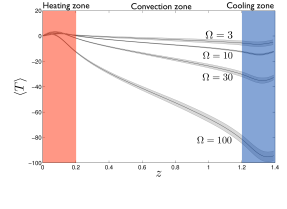
Figure 1.— Top: Steady-state temperature profiles in four simulations (labelled 3M, 10M, 30L and 100L in Table 1) with different values of $\Omega$, averaged over horizontal planes and in time. The shading around each curve represents the corresponding RMS fluctuation. Temporal averaging is over at least 50 time units. Bottom: The black lines show the slopes of the four profiles in the top panel. Also shown as colored points are comparison simulations with higher diffusivities (blue for ones labelled M in Table 1 and light blue if labelled H). Our simulation units throughout this paper are determined by setting $F=H=1$.

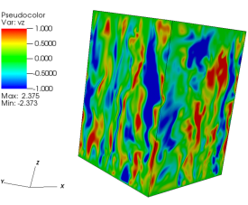
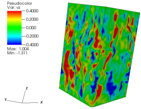
Figure 2.— Vertical velocity in a simulation with $\Omega=10$ (left panel; simulation 10M) and $\Omega=1000$ (right panel; 1000L), both at $t=50$. In the right panel, the horizontal scale of the box has been stretched by a factor of $100^{3/5}$ relative to the left panel, and the colour scale has similarly been scaled by $100^{-1/5}$. These scalings correspond with the predictions in §3.

The top panel of Fig. 1 shows the averaged temperature profiles in steady state for four simulations with different rotation rates. The temperature gradient in the convection zone steepens as $\Omega$ is increased. That is because rotation hinders convection: to achieve a given flux ($F=1$) requires a steeper gradient in a more rapidly rotating simulation. The bottom panel of Fig. 1 shows the slopes of the profiles in the top panel (black curves), along with those from simulations with higher diffusivities (colored points). The fact that the points agree with the curves shows that we are probing the regime in which the bulk properties are independent (or at worst weakly dependent) on the microscopic diffusion coefficients.

Fig. 2 shows a snapshot of $v_{z}$ in two simulations, one with $\Omega=10$ and the other with $\Omega=1000$. For the right panel, we scaled the horizontal length scale, as well as the colour scale, by the amount predicted by the arguments in §3, relative to the left panel. The similarity of the flow in both panels provides support for the mixing length theory. The dominant convective modes occur on smaller horizontal length-scales for more rapid rotation (Eq. 15), and the corresponding vertical velocities decrease (Eq. 13).

Fig. 3 shows the spectrum of the heat flux in three $\Omega=10$ simulations that have different diffusivities. The heat flux in these simulations is dominated by wavenumbers near $k_{\perp}\sim 20-30$. When $\nu$ and $\kappa$ are decreased, the spectrum does not change near those lengthscales, indicating that the modes that dominate the heat flux are well-resolved and hence bulk properties are independent of $\nu$ and $\kappa$. The convection is anisotropic, since the depth of the convection zone is considerably larger than the scale of modes that dominate the heat flux. This anisotropy is evident in Fig. 2, and is expected from linear theory (Eq. 8). We also deduce from Fig. 3 that when $\nu$ is decreased, the inertial range is extended to smaller scales. But those small scales have little influence on the larger scales that carry the bulk of the heat transport. These deductions conform with the expectation from §3.

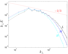
Figure 3.— Spectrum of the heat flux for three simulations with $\Omega=10$ and different viscosities. The ordinate is $k_{\perp}E(k_{\perp})=k_{\perp}^{2}\mathrm{Re}\left<\hat{v}_{z}(\mbox{\boldmath$k$\unboldmath}_{\perp},z,t)\hat{T}(\mbox{\boldmath$k$\unboldmath}_{\perp},z,t)^{*}\right>$ (within a constant), where hats denote Fourier transforms in the horizontal directions with horizontal wavevector $k_{\perp}$, and the averaging is threefold: (i) over $z$ inside the convection zone; (ii) over the orientation of $\mbox{\boldmath$k$\unboldmath}_{\perp}$; and (iii) over time until convergence. Note that the spatially averaged flux is $F={\rm const}\times\int E(k_{\perp})dk_{\perp}$, so that the peak of the spectrum plotted indicates the wavenumbers that dominate the flux. The $-2/3$ line corresponds to the Kolmogorov scaling, i.e., the assumption that fluctuations across lengthscale $\lambda_{\perp}$ scale as $\delta v_{z},\delta T\propto\lambda_{\perp}^{1/3}$, and that the two are strongly correlated. The jaggedness is due to the discrete nature of the simulation grid, not temporal fluctuations which have been averaged away.

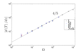
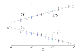
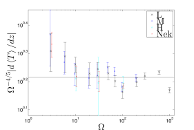
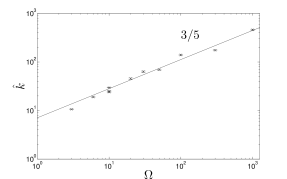
Figure 4.— Dependence of bulk properties on rotation rate. The predictions from mixing length theory are shown as lines. The points labelled L, M, and H are SNOOPY simulations with viscosities from low to high; red points are Nek5000 results; and error bars are RMS fluctuations. Points with the same $\Omega$ are slightly offset horizontally for clarity. Our simulation units are determined by setting $F=H=1$.

Figure 4, the main result of this paper, displays the bulk properties in all of the simulations listed in Table 1. The top-left panel shows the average temperature gradient in the convection zone, which we extract by fitting the temporally and horizontally averaged temperature profile in the central $\frac{1}{3}$ of the simulation domain with a straight line. The gradient is shown as a point and the corresponding RMS fluctuation as error bars, after averaging over at least 50 time units. At each $\Omega$, the results from the different simulations—SNOOPY with various viscosities and Nek—agree quite well with the prediction, shown as a solid line. We fit the points and RMS errors for all simulations with a linear least squares fit in log-log space, keeping points with $\Omega>6$ only (i.e. the rapidly rotating limit). We find

$$-{d\left<T\right>\over dz}=1.9^{+0.3}_{-0.3}\;\Omega^{0.75\pm 0.06}.$$ (17)

The exponent agrees with the theoretical prediction of 0.8 (Eq. 12) within the error bars. The lower-left panel of Fig. 4 plots the same data after removing the predicted scaling. The prediction works remarkably well over more than two orders of magnitude; exponents that differ from 0.8 by more than $\sim 10\%$ are definitively ruled out.

The top-right panel of Fig. 4 shows the RMS fluctuations in $v_{z}$ and $T$ at the midplane of the box $(z=L_{z}/2)$. These also agree very well with the predicted scalings, shown as lines. A least-squares fit to the simulation points gives

$$\delta v_{z} = 0.9^{+0.5}_{-0.3}\;\Omega^{-0.15\pm 0.08}\ ,$$ (18)

$$\delta T = 1.5^{+0.9}_{-0.6}\;\Omega^{0.21\pm 0.13}\ ,$$ (19)

the exponents of which may be compared with the predictions of -0.2 for $\delta v_{z}$ (Eq. 13), and +0.2 for $\delta T$ (Eq. 14).

In the fourth panel of Fig. 4, we plot the horizontal wavenumber that dominates the heat flux, $\hat{k}$. We define it via

$$\hat{k}={\int k_{\perp}E(k_{\perp})d\ln k_{\perp}\over\int E(k_{\perp})d\ln k_{\perp}}\ ,$$ (20)

where the flux spectrum $E(k_{\perp})$ is defined in the caption of Fig. 3. Note that both the numerator and denominator of this expression are dominated by large scales. A least-squares fit to the plotted values yields

$$\hat{k}=7.3^{+7.2}_{-3.6}\;\Omega^{0.58\pm 0.19}\ ,$$ (21)

which may be compared with the mixing length prediction $k_{\perp}\propto\Omega^{0.6}$ (Eq. 15).

The results of this section, and in particular Fig. 4, provides strong support for the mixing length theory presented in §2.

5. Simulations Without Internal Heating and Cooling

For the simulations presented in §4, we directly heated and cooled the fluid inside the simulation domain to avoid thin boundary layers. That approach was predicated on the assumption that the details of how heat enters and leaves the convection zone is only of minor importance for determining the bulk properties. In this section, we test that assumption. To do so, we run comparison simulations without any internal heating or cooling. The temperature is held fixed at the bottom boundary and the flux is fixed at the top, which is essentially the setup for standard Rayleigh-Benard convection. Since the fluid is driven by heating at the boundaries, it is essential to correctly resolve the thermal boundary layers – failing to do so results in an incorrect heat flux through the domain (Groetzbach, 1983; Shishkina et al., 2010). When the diffusivities are small, the boundary layers become very thin, and hence computationally costly to resolve.

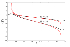
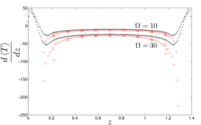
Figure 5.— Temperature profiles in simulations with (black) and without (red) internal heating at two rotation rates. Those with internal heating are 10M and 30M. The ones with no internal heating were done with Nek5000. The temperature was fixed at the bottom and the flux fixed at the top to $F=1$. We set $L_{z}=1.2$ in order to crudely account for the fact that in the internally heated simulations the convection zone extends somewhat into the heating/cooling zones. The simulation without internal heating that has $\Omega=10$ also has $L_{\perp}=1$, $\nu=\kappa=10^{-3}$, and uses $200^{3}$ points split into 20 elements and 10th order polynomials within each element per dimension; the simulation with $\Omega=30$ has $L_{\perp}=0.5$, $\nu=\kappa=10^{-3.6}$, and similarly uses $200^{3}$ points.

The equations of motion (Eqs. A1–A2 with $q=0$) were integrated with Nek5000, which is better suited than SNOOPY for resolving thin boundary layers. This is because grid points in Nek5000 are clustered towards the boundaries, whereas in SNOOPY sharp boundary layers produce unwanted Gibbs oscillations. Fig. 5 shows the temperature profiles and gradients from two such simulations, with $\Omega=10$ and 30, and compares them with the corresponding heating/cooling zone simulations. The agreement is reasonable throughout the convection zone, thus confirming our assumption. The thin boundary layers are also evident in these figures.

6. Discussion

We presented a simple derivation of mixing length theory in rapidly rotating convection, and then verified it with simulations. The theory, postulated by Stevenson (1979), predicts the properties of the convecting fluid under the assumption that they are independent of microscopic diffusivities ($\nu$ and $\kappa$). Equations 12–15 list the predictions for the mean temperature gradient, the velocity and temperature fluctuations, and the lengthscale of the modes that dominate heat transport. Our simulation results, summarized in Figure 4, agree remarkably well with the theory, across more than two orders of magnitude in rotation rate.

We chose to focus on a very simple setup: Boussinesq convection in a box. But despite its simplicity, and despite the vast literature already devoted to the topic, the result remains under debate (e.g., King et al., 2012; Julien et al., 2012), largely because of the complicating effect of boundary layers. We circumvented this complication by focusing on the properties of the convecting fluid—i.e., between the boundary layers. We did this by fixing the flux, and examining the interior fluid’s properties for increasingly small diffusivities. We thereby showed that the convecting fluid’s properties converged to the prediction of mixing length theory as $\nu$, $\kappa\rightarrow 0$. Moreover, the numerical resolutions required to demonstrate convergence were relatively modest, after artificially thickening the boundary layers with heating/cooling zones. For example, our SNOOPY simulations had 256³ gridpoints or fewer. Our numerical results provide strong support for those of Julien et al. (2012), who simulate a set of reduced equations valid in the limit of rapid rotation.

Our work lends confidence to mixing length theory’s ability to accurately model highly turbulent convection. We hope to extend it to include a variety of more complicated—and realistic—effects, some of the most important of which are as follows:

• Including a background density gradient. One must then distinguish between entropy and temperature. The argument presented in §3 should remain largely unchanged, after replacing temperature with entropy. But a possible complication is the asymmetry between upflows and downflows in the presence of a density gradient (e.g. Hurlburt et al. 1984; Cattaneo et al. 1991; Miesch 2005).

• Allowing for a more realistic geometry, i.e., quasi-spherical rather than cubical. The work presented in this paper strictly applies only to a small patch of the convective region near the poles of the star or planet. An intermediate step before considering the full spherical problem would be to allow rotation and gravity to be misaligned. Stevenson (1979) predicts that in that case Eqs. 12–15 should be altered by replacing $\Omega\rightarrow\Omega\cos\theta$, where $\theta$ is co-latitude. But that has yet to be confirmed by simulations.

• Including the boundaries of a convection zone and the possibilities of penetration and overshooting into neighbouring stable layers (e.g. Hurlburt et al. 1994; Brummell et al. 2002; Rogers & Glatzmaier 2005)

• Allowing for the interaction between convection and differential rotation, and the generation of secondary flows.

• Including magnetic fields.

A large body of work has already been devoted to simulations of convection in rotating stars and planets, from Boussinesq (e.g. Hathaway & Somerville 1983; Schmitz & Tilgner 2009; King et al. 2012) to fully compressible (Brummell et al., 1996, 1998; Käpylä et al., 2005) Cartesian box simulations to Boussinesq (Christensen, 2002; Christensen & Aubert, 2006), anelastic (Glatzmaier, 1984; Miesch et al., 2000; Kaspi et al., 2009; Jones & Kuzanyan, 2009; Gastine & Wicht, 2012) and fully compressible simulations (Käpylä et al., 2011) in spherical shell geometry. Given the evident complexities of some of these simulations, it is our view that a more complete understanding of simpler models is required to enable us to understand these simulation results. Our work complements the literature by definitively verifying the rotating mixing length theory described in §3 for the case of Boussinesq convection in the polar regions of a planet or star. We anticipate that the theory described in this paper, as well as the extensions discussed above, will help provide a theoretical basis for the simulation results.

Turning to astrophysical applications of the theory, we note first that rotation changes the entropy gradient relative to that predicted by standard (non-rotating) mixing length theory by an order-unity factor—at least for the Sun, where the rotation rate is comparable to the convective turnover time. Thus the inclusion of rotation will not substantially change static structure calculations, since it hardly affects the conclusion that convection zones have a near-constant entropy throughout (Stevenson, 1979). But a potentially important application is explaining the differential rotation profile of the Sun and other stars. In particular, small latitudinal entropy gradients drive differential rotation via the thermal wind equation (e.g. Thompson et al. 2003; Miesch et al. 2006; Balbus 2009; Balbus et al. 2009). Therefore to predict the differential rotation profile from first principles requires one to understand how the entropy gradient depends on latitude. It appears likely that rotating mixing length theory (at least when extended to the case in which rotation and gravity are misaligned) will provide an important piece towards solving this puzzle.

Another potential application is to tidal dissipation in a convective star or planet that has an orbiting companion. This is important for understanding, for example, the tidal circularization of solar-type binary stars out to approximately ten day orbits. Previous work estimates the turbulent viscosity due to convection by employing non-rotating mixing length theory (Zahn, 1966; Goldreich & Nicholson, 1977). It would be of interest to see how the predictions are affected by employing rotating mixing length theory.

Appendix A Numerical Methods

A.1. Convection with Heating/Cooling Zones (SNOOPY)

The majority of our simulations use SNOOPY (Lesur & Longaretti 2005; Lesur & Ogilvie 2010), a Cartesian pseudo-spectral code. We use it to evolve the following equations of motion,

$$\left(\partial_{t}+\boldsymbol{v}\cdot\nabla\right)\boldsymbol{v}+2\Omega\boldsymbol{e}_{z}\times\boldsymbol{v} = -\nabla p+T\boldsymbol{e}_{z}+\nu\nabla^{2}\mbox{\boldmath$v$\unboldmath},\ \ \$$ (A1)

$$\left(\partial_{t}+\boldsymbol{v}\cdot\nabla\right)T = q+\kappa\nabla^{2}T,$$ (A2)

which are modified from the strict Boussinesq equations (Eqs. 2–3) by the inclusion of diffusive terms and a spatially variable heating/cooling function $q(z)$. Rather than evolving $T$ directly, we write

$$T=-\beta z+\theta,$$ (A3)

with $\beta$ a constant, and evolve $\theta$. We describe below our choices for $\beta$ and $q$. Table 1 lists all of our heating/cooling simulations.

Throughout this paper we take $\nu=\kappa$, with a value as small as possible for a given number of grid points, subject to the constraint that the bulk properties be numerically well resolved. Our computational domain is a Cartesian box with dimensions $x,y\in[0,L_{\perp}]$ and $z\in[0,L_{z}]$, with $L_{z}=1.4$ throughout. We vary $L_{\perp}$ until we have resolved the dominant convective scales, using intuition from linear theory (Chandrasekhar, 1961) and analysis of the horizontal energy spectrum. We verify that the bulk properties are independent of this parameter, once it is sufficiently large to capture the dominant convective modes.

Boundary conditions in the horizontal direction are periodic, and in the vertical direction are impermeable ($v_{z}=0$), stress-free ($\partial_{z}v_{x}=\partial_{z}v_{y}=0$), and constant temperature ($\theta=0$) at the top and bottom ($z=0$ and $L_{z}$). Note that we evolve $\theta$ rather than $T$ because it allows us to impose the vertical boundary conditions on $\theta$ with a sine-wave decomposition.

Table 1Simulation Parameters

Label	$\Omega$	$L_{\perp}$	$-\log_{10}{\nu}$	$N$	$v_{z}$	$|\frac{d\langle T\rangle}{dz}|$	Ro$=v_{z}/(2\Omega H)$	E$=\nu/(2\Omega H^{2})$	$\mathrm{Ra}_{f}=FH^{4}/\nu^{3}$	Nu$=F/(\nu|\frac{d\langle T\rangle}{dz}|)$
3M	3	2	3	128	0.72$\pm 0.05$	5.5$\pm 1.2$	$0.12$	$1.7\times 10^{-4}$	$1.0\times 10^{9}$	183
3L	3	2	2.7	192	0.70$\pm 0.06$	4.9$\pm 0.75$	$0.12$	$3.3\times 10^{-4}$	$1.3\times 10^{8}$	102
3Nek	3	2	3	20$\times$10	0.72$\pm 0.05$	5.4$\pm 0.55$	$0.12$	$1.7\times 10^{-4}$	$1.0\times 10^{9}$	186
6M	6	1.5	2.6	128	0.62$\pm 0.05$	7.6$\pm 0.7$	$5.2\times 10^{-2}$	$2.1\times 10^{-4}$	$6.3\times 10^{7}$	53
6L	6	1.2	3.1	192	0.66$\pm 0.06$	8.2$\pm 1.0$	$5.5\times 10^{-2}$	$6.6\times 10^{-5}$	$2.0\times 10^{9}$	154
10H	10	1	3	128	0.61$\pm 0.06$	10.5$\pm 1.0$	$3.0\times 10^{-2}$	$5.0\times 10^{-5}$	$1.0\times 10^{9}$	95
10M	10	1	3.15	192	0.64$\pm 0.06$	10.4$\pm 0.95$	$3.2\times 10^{-2}$	$3.5\times 10^{-5}$	$2.8\times 10^{9}$	136
10L	10	1	3.3	256	0.61$\pm 0.05$	11.5$\pm 0.7$	$3.0\times 10^{-2}$	$2.5\times 10^{-5}$	$7.9\times 10^{9}$	174
10Nek	10	1	3	20$\times$10	0.60$\pm 0.05$	10.9$\pm 0.9$	$3.0\times 10^{-2}$	$5.0\times 10^{-5}$	$1.0\times 10^{9}$	92
20M	20	0.7	3.3	128	0.57$\pm 0.06$	17.5$\pm 1.4$	$1.4\times 10^{-2}$	$1.3\times 10^{-5}$	$7.9\times 10^{9}$	114
20L	20	0.7	3.55	192	0.60$\pm 0.06$	18.6$\pm 1.7$	$1.5\times 10^{-2}$	$7.0\times 10^{-6}$	$4.5\times 10^{10}$	191
30H	30	0.3	3.5	128	0.52$\pm 0.07$	24.4$\pm 5.7$	$8.6\times 10^{-3}$	$5.3\times 10^{-6}$	$3.2\times 10^{10}$	130
30M	30	0.4	3.8	192	0.57$\pm 0.08$	24.7$\pm 2.5$	$9.5\times 10^{-3}$	$2.6\times 10^{-6}$	$2.5\times 10^{11}$	255
30L	30	0.4	4.05	256	0.58$\pm 0.07$	26.7$\pm 1.5$	$9.7\times 10^{-3}$	$1.5\times 10^{-6}$	$1.4\times 10^{12}$	420
30Nek	30	0.6	3.5	20$\times$10	0.53$\pm 0.06$	25.1$\pm 2.1$	$8.9\times 10^{-3}$	$5.3\times 10^{-6}$	$3.2\times 10^{10}$	126
50M	50	0.5	3.5	128	0.46$\pm 0.04$	39.7$\pm 1.7$	$4.6\times 10^{-3}$	$3.2\times 10^{-6}$	$3.2\times 10^{10}$	80
50L	50	0.4	4.2	256	0.53$\pm 0.06$	38.8$\pm 2.1$	$5.3\times 10^{-3}$	$6.3\times 10^{-7}$	$4.0\times 10^{12}$	409
70M	70	0.4	3.5	128	0.43$\pm 0.04$	50.4$\pm 1.7$	$3.0\times 10^{-3}$	$2.3\times 10^{-6}$	$3.2\times 10^{10}$	63
70L	70	0.35	3.75	192	0.46$\pm 0.05$	47.6$\pm 2.2$	$3.3\times 10^{-3}$	$1.3\times 10^{-6}$	$1.8\times 10^{11}$	118
100H	100	0.2	3.5	128	0.38$\pm 0.05$	63.9$\pm 3.5$	$1.9\times 10^{-3}$	$1.6\times 10^{-6}$	$3.2\times 10^{10}$	49
100M	100	0.2	4	192	0.45$\pm 0.05$	59.0$\pm 2.2$	$2.2\times 10^{-3}$	$5.0\times 10^{-7}$	$1.0\times 10^{12}$	170
100L	100	0.2	4.3	192	0.51$\pm 0.07$	58.0$\pm 3.0$	$2.6\times 10^{-3}$	$2.5\times 10^{-7}$	$7.9\times 10^{12}$	344
100Nek	100	0.2	3.5	20$\times$10	0.39$\pm 0.03$	63.4$\pm 1.2$	$2.0\times 10^{-3}$	$1.6\times 10^{-6}$	$3.2\times 10^{10}$	50
200M	200	0.15	3.75	128	0.33$\pm 0.04$	111$\pm 3.2$	$8.0\times 10^{-4}$	$4.4\times 10^{-7}$	$1.8\times 10^{11}$	51
200L	200	0.15	4	128	0.36$\pm 0.05$	110$\pm 4.0$	$9.0\times 10^{-4}$	$2.5\times 10^{-7}$	$1.0\times 10^{12}$	91
300L	300	0.2	4	128	0.33$\pm 0.03$	160$\pm 4.2$	$5.4\times 10^{-4}$	$1.7\times 10^{-7}$	$1.0\times 10^{12}$	63
600L	600	0.1	4.35	128	0.29$\pm 0.03$	286$\pm 4.6$	$2.4\times 10^{-4}$	$3.7\times 10^{-8}$	$1.1\times 10^{13}$	78
1000L	1000	0.05	4.7	128	0.28$\pm 0.04$	372$\pm 7.8$	$1.4\times 10^{-4}$	$1.0\times 10^{-8}$	$1.3\times 10^{14}$	135

Our $q$ (Fig. 6) is chosen so that fluid is heated at the bottom of the box in a zone of depth $\Delta=0.2$, and cooled by an equal amount at the top. In addition, $q=0$ in the central convection zone, which has depth $H=1$. Explicitly,

$$q(z)=\frac{1}{\Delta}\begin{cases}1+\cos\left(\frac{2\pi(z-\Delta/2)}{\Delta}\right)&\text{if }0\leq z\leq\Delta,\\ 0&\text{if }\Delta<z<L_{z}-\Delta,\\ -1-\cos\left(\frac{2\pi(z-L_{z}+\Delta/2)}{\Delta}\right)&\text{if }L_{z}-\Delta\leq z\leq L_{z},\\ \end{cases}$$

which has integrated heating at the bottom

$$\int_{0}^{\Delta}q(z)dz=1\ ,$$ (A4)

and an equal amount of cooling at the top. This gives unit flux in the convection zone in steady state, as long as the flux vanishes at the top and bottom edges of the simulation box.

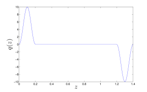
Figure 6.— Internal heating and cooling profile used in our simulations. The convection zone is the region $z\in[0.2,1.2]$, where $q(z)=0$.

The value of $\beta$ is chosen to achieve zero flux at the box edges, using a relaxation method. Specifically, it is straightforward to show that for the flux to vanish at the top and bottom edges one must have in steady state

$$\kappa\beta L_{z}=L_{z}-\Delta-\int_{0}^{L_{z}}\left<v_{z}\theta\right>dz,$$ (A5)

where the angled brackets here denote an average across a horizontal plane, as well as in time, and we have used the boundary conditions to eliminate some terms. We evaluate the right-hand side of Eq. A5 in the code to give a target value for $\beta$, which we call $\tilde{\beta}$, and relax $\beta$ towards its target value by solving

$$\frac{d\beta}{dt}=\frac{1}{\tau}\left(\tilde{\beta}-\beta\right),$$ (A6)

where $\tau$ is typically a few hundred in code units. The simulation proceeds until Eq. A5 is satisfied within 1%. After that, $\beta$ is held fixed. In some of the simulations, turbulent fluctuations are sufficiently large that the relaxation method is never switched off according to the above criterion. This leads to slow and small changes in $\beta$. By rerunning some of these simulations with the relaxation method turned off, we found that these slow, small changes do not appreciably change the mean properties (but they can amplify fluctuations by $\sim 50\%$).

We integrate the equations of motion with a first order splitting method, made up of an implicit step for $q(z)$ and the diffusive terms, and an explicit third order Runge-Kutta method for all other terms. The implicit step uses an integrating factor to write the solution for a given Fourier mode at time $t_{n}$ as

$$\hat{\theta}(\boldsymbol{k},t_{n})=\hat{\theta}(\boldsymbol{k},t_{n-1})e^{-\kappa k^{2}\delta t}+\frac{\hat{q}(\boldsymbol{k})}{\kappa k^{2}}\left(1-e^{-\kappa k^{2}\delta t}\right),$$ (A7)

where $\hat{q}$ is the discrete Fourier transform of $q$ and $\delta t$ is the time step. This allows larger timesteps to be used than with a fully explicit method.

A.2. Nek5000

We have also run a number simulations with Nek5000, an efficiently parallelised spectral element code (Fischer et al., 2008). For the simulations described in §4 with heating/cooling zones, the setup is almost the same as for the SNOOPY simulations described above, except we evolve $T$ directly rather than $\theta$. In addition, we impose zero flux ($\partial_{z}T=0$) conditions at each point on the top and bottom edges of the simulation box, rather than the constant temperature boundary condition in SNOOPY. We also use explicit second-order time integration for the heating and cooling terms, whereas diffusive terms are integrated using an implicit method of the same order. The convective terms are fully de-aliased using the 3/2 rule, so that the polynomial order listed in Table. 1 is actually $15$ (not 10) for the integration of these terms. The simulations with Nek5000 agree well with those done with SNOOPY (see Fig. 4), which provides an independent check on our results.

References

- Ahlers et al. (2009) Ahlers, G., Grossmann, S., & Lohse, D. 2009, Reviews of Modern Physics, 81, 503
- Aubert et al. (2001) Aubert, J., Brito, D., Nataf, H.-C., Cardin, P., & Masson, J.-P. 2001, Physics of the Earth and Planetary Interiors, 128, 51
- Balbus (2009) Balbus, S. A. 2009, MNRAS, 395, 2056
- Balbus et al. (2009) Balbus, S. A., Bonart, J., Latter, H. N., & Weiss, N. O. 2009, MNRAS, 400, 176
- Böhm-Vitense (1958) Böhm-Vitense, E. 1958, Zeitschrift für Astrophysik, 46, 108
- Brummell et al. (2002) Brummell, N. H., Clune, T. L., & Toomre, J. 2002, ApJ, 570, 825
- Brummell et al. (1996) Brummell, N. H., Hurlburt, N. E., & Toomre, J. 1996, ApJ, 473, 494
- Brummell et al. (1998) —. 1998, ApJ, 493, 955
- Cattaneo et al. (1991) Cattaneo, F., Brummell, N. H., Toomre, J., Malagoli, A., & Hurlburt, N. E. 1991, ApJ, 370, 282
- Chandrasekhar (1961) Chandrasekhar, S. 1961, Hydrodynamic and hydromagnetic stability
- Christensen (2002) Christensen, U. R. 2002, Journal of Fluid Mechanics, 470, 115
- Christensen & Aubert (2006) Christensen, U. R., & Aubert, J. 2006, Geophysical Journal International, 166, 97
- Fischer et al. (2008) Fischer, P. F., Lottes, J. W., & Kerkemeier, S. G. 2008, nek5000 Web page, http://nek5000.mcs.anl.gov
- Garaud et al. (2010) Garaud, P., Ogilvie, G. I., Miller, N., & Stellmach, S. 2010, MNRAS, 407, 2451
- Gastine & Wicht (2012) Gastine, T., & Wicht, J. 2012, Icarus, 219, 428
- Gillet & Jones (2006) Gillet, N., & Jones, C. A. 2006, Journal of Fluid Mechanics, 554, 343
- Glatzmaier (1984) Glatzmaier, G. A. 1984, Journal of Computational Physics, 55, 461
- Goldreich & Nicholson (1977) Goldreich, P., & Nicholson, P. D. 1977, Icarus, 30, 301
- Groetzbach (1983) Groetzbach, G. 1983, Journal of Computational Physics, 49, 241
- Grossmann & Lohse (2000) Grossmann, S., & Lohse, D. 2000, Journal of Fluid Mechanics, 407, 27
- Hathaway & Somerville (1983) Hathaway, D. H., & Somerville, R. C. J. 1983, Journal of Fluid Mechanics, 126, 75
- Hide (1974) Hide, R. 1974, Royal Society of London Proceedings Series A, 336, 63
- Hurlburt et al. (1984) Hurlburt, N. E., Toomre, J., & Massaguer, J. M. 1984, ApJ, 282, 557
- Hurlburt et al. (1994) Hurlburt, N. E., Toomre, J., Massaguer, J. M., & Zahn, J.-P. 1994, ApJ, 421, 245
- Jones & Kuzanyan (2009) Jones, C. A., & Kuzanyan, K. M. 2009, Icarus, 204, 227
- Julien et al. (2012) Julien, K., Knobloch, E., Rubio, A. M., & Vasil, G. M. 2012, Physical Review Letters, 109, 254503
- Käpylä et al. (2005) Käpylä, P. J., Korpi, M. J., Stix, M., & Tuominen, I. 2005, A& A, 438, 403
- Käpylä et al. (2011) Käpylä, P. J., Mantere, M. J., Guerrero, G., Brandenburg, A., & Chatterjee, P. 2011, A& A, 531, A162
- Kaspi et al. (2009) Kaspi, Y., Flierl, G. R., & Showman, A. P. 2009, Icarus, 202, 525
- King et al. (2012) King, E. M., Stellmach, S., & Aurnou, J. M. 2012, Journal of Fluid Mechanics, 691, 568
- King et al. (2013) King, E. M., Stellmach, S., & Buffett, B. 2013, Journal of Fluid Mechanics, 717, 449
- King et al. (2009) King, E. M., Stellmach, S., Noir, J., Hansen, U., & Aurnou, J. M. 2009, Nature, 457, 301
- Kraichnan (1962) Kraichnan, R. H. 1962, Physics of Fluids, 5, 1374
- Lesur & Longaretti (2005) Lesur, G., & Longaretti, P.-Y. 2005, A&A, 444, 25
- Lesur & Ogilvie (2010) Lesur, G., & Ogilvie, G. I. 2010, MNRAS, 404, L64
- Lohse & Toschi (2003) Lohse, D., & Toschi, F. 2003, Physical Review Letters, 90, 034502
- Malkus (1954) Malkus, W. V. R. 1954, Royal Society of London Proceedings Series A, 225, 196
- Miesch (2005) Miesch, M. S. 2005, Living Reviews in Solar Physics, 2, 1
- Miesch et al. (2006) Miesch, M. S., Brun, A. S., & Toomre, J. 2006, ApJ, 641, 618
- Miesch et al. (2000) Miesch, M. S., Elliott, J. R., Toomre, J., et al. 2000, ApJ, 532, 593
- Niemela & Sreenivasan (2010) Niemela, J. J., & Sreenivasan, K. R. 2010, New Journal of Physics, 12, 115002
- Rogers & Glatzmaier (2005) Rogers, T. M., & Glatzmaier, G. A. 2005, ApJ, 620, 432
- Schmitz & Tilgner (2009) Schmitz, S., & Tilgner, A. 2009, Phys. Rev. E, 80, 015305
- Shishkina et al. (2010) Shishkina, O., Stevens, R. J. A. M., Grossmann, S., & Lohse, D. 2010, New Journal of Physics, 12, 075022
- Showman et al. (2011) Showman, A. P., Kaspi, Y., & Flierl, G. R. 2011, Icarus, 211, 1258
- Shraiman & Siggia (1990) Shraiman, B. I., & Siggia, E. D. 1990, PRA, 42, 3650
- Spiegel (1971) Spiegel, E. A. 1971, ARA& A, 9, 323
- Spiegel & Veronis (1960) Spiegel, E. A., & Veronis, G. 1960, ApJ, 131, 442
- Stevenson (1979) Stevenson, D. J. 1979, Geophysical and Astrophysical Fluid Dynamics, 12, 139
- Thompson et al. (2003) Thompson, M. J., Christensen-Dalsgaard, J., Miesch, M. S., & Toomre, J. 2003, ARA& A, 41, 599
- Zahn (1966) Zahn, J. P. 1966, Annales d’Astrophysique, 29, 489