LINVIEW: Incremental View Maintenance
for Complex Analytical Queries

Abstract

Many analytics tasks and machine learning problems can be naturally expressed by iterative linear algebra programs. In this paper, we study the incremental view maintenance problem for such complex analytical queries. We develop a framework, called Linview, for capturing deltas of linear algebra programs and understanding their computational cost. Linear algebra operations tend to cause an avalanche effect where even very local changes to the input matrices spread out and infect all of the intermediate results and the final view, causing incremental view maintenance to lose its performance benefit over re-evaluation. We develop techniques based on matrix factorizations to contain such epidemics of change. As a consequence, our techniques make incremental view maintenance of linear algebra practical and usually substantially cheaper than re-evaluation. We show, both analytically and experimentally, the usefulness of these techniques when applied to standard analytics tasks. Our evaluation demonstrates the efficiency of Linview in generating parallel incremental programs that outperform re-evaluation techniques by more than an order of magnitude.

1 Introduction

Linear algebra plays a major role in modern data analysis. Many state-of-the-art data mining and machine learning algorithms are essentially linear transformations of vectors and matrices, often expressed in the form of iterative computation. Data practitioners, engineers, and scientists utilize such algorithms to gain insights about the collected data.

Data processing has become increasingly expensive in the era of big data. Computational problems in many application domains, like social graph analysis, web analytics, and scientific simulations, often have to process petabytes of multidimensional array data. Popular statistical environments, like R and MATLAB, offer high-level abstractions that simplify programming but lack the support for scalable full-dataset analytics. Recently, many scalable frameworks for data analysis have emerged: MADlib [18] and Columbus [36] for in-database scalable analytics, SciDB [32], SciQL [39], and RasDaMan [4] for in-database array processing, Mahout and MLbase [22] for machine learning and data mining on Hadoop and Spark [35]. High-performance computing relies on optimized libraries, like Intel MKL and ScaLAPACK, to accelerate the performance of matrix operations in data-intensive computations. All these solutions primarily focus on efficiently processing large volumes of data.

Modern applications have to deal with not just big, but also rapidly changing datasets. A broad range of examples including clickstream analysis, algorithmic trading, network monitoring, and recommendation systems compute realtime analytics over streams of continuously arriving data. Online and responsive analytics allow data miners, analysts, and statisticians to promptly react to certain, potentially complex, conditions in the data; or to gain preliminary insights from approximate or incomplete results at very early stages of the computation. Existing tools for large-scale data analysis often lack support for dynamic datasets. High data velocity forces application developers to build ad hoc solutions in order to deliver high performance. More than ever, data analysis requires efficient and scalable solutions to cope with the ever-increasing volume and velocity of data.

Most datasets evolve through changes that are small relative to the overall dataset size. For example, the Internet activity of a single user, like a user’s purchase history or movie ratings, represents only a tiny portion of the collected data. Recomputing data analytics on every (moderate) dataset change is far from efficient.

These observations motivate incremental data analysis. Incremental processing combines the results of previous analyses with incoming changes to provide a computationally cheap method for updating the result. The underlying assumption that these changes are relatively small allows us to avoid re-evaluation of expensive operations. In the context of databases, incremental processing – also known as incremental view maintenance – reduces the cost of query evaluation by simplifying or eliminating join processing for changes in the base relations [17, 21]. However, simulating multidimensional array computations on top of traditional RDBMSs can result in poor performance [32]. Data stream processing systems [27, 1] also rely on incremental computation to reduce the work over finite windows of input data. Their usefulness is yet limited by their window semantics and inability to handle long-lived data.

In this work we focus on incremental maintenance of analytical queries written as (iterative) linear algebra programs. A program consists of a sequence of statements performing operations on vectors and matrices. For each matrix (vector) that dynamically changes over time, we define a trigger program describing how an incremental update affects the result of each statement (materialized view). A delta expression of one statement captures the difference between the new and old result. This paper shows how to propagate delta expressions through subsequent statements while avoiding re-evaluation of computationally expensive operations, like matrix multiplication or inversion.

Example 1.1

Consider the program that computes the fourth power of a given matrix $A$.

B := A A;C := B B; The goal is to maintain the result $C$ on every update of $A$ by $\Delta{A}$. We compare the time complexity of two computation strategies: re-evaluation and incremental maintenance. The re-evaluation strategy first applies $\Delta{A}$ to $A$ and then performs two $\mathcal{O}(n^{3})$ matrix multiplications to update $C$.

The incremental approach exploits the associativity and distributivity of matrix multiplication to compute a delta expression for each statement of the program. The trigger program for updates to $A$ is:

ON UPDATE A BY $\Delta$A:    $\Delta$B := ($\Delta$A)A + A($\Delta$A) + ($\Delta$A)($\Delta$A);    $\Delta$C := ($\Delta$B)B + B($\Delta$B) + ($\Delta$B)($\Delta$B);    A += $\Delta$A;  B += $\Delta$B;  C += $\Delta$C; Let us assume that $\Delta{A}$ represent a change of one cell in $A$. Fig. 1 shows the effect of that change on $\Delta{B}$ and $\Delta{C}$ . The shaded regions represent entries with nonzero values. The incremental approach capitalizes on the sparsity of $\Delta{A}$ and $\Delta{B}$ to compute $\Delta{B}$ and $\Delta{C}$ in $\mathcal{O}(n)$ and $\mathcal{O}(n^{2})$ operations, respectively. Together with the cost of updating $B$ and $C$, incremental evaluation of the program requires $\mathcal{O}(n^{2})$ operations, clearly cheaper than re-execution. $\Box$

The main challenge in incremental linear algebra is how to represent and propagate delta expressions. Even a small change in a matrix (e.g., a change of one entry) might have an avalanche effect that updates every entry of the result matrix. In Example 1.1, a single entry change in $A$ causes changes of one row and column in $B$, which in turn pollute the entire matrix $C$. If we were to propagate $\Delta{C}$ to a subsequent expression – for example, the expression $D=C\,C$ that computes $A^{8}$ – then evaluating $\Delta{D}$ would require two full $\mathcal{O}(n^{3})$ matrix multiplications, which is obviously more expensive than recomputing $D$ using the new value of $C$.

To confine the effect of such changes and allow efficient evaluation, we represent delta expressions in a factored form, as products of low-rank matrices. For instance, we could represent $\Delta{B}$ as a vector outer product for single entry updates in $A$. Due to the associativity and distributivity of matrix multiplication, the factored form allows us to choose the evaluation order that completely avoids expensive matrix multiplications.

To the best of our knowledge, this is the first work done towards efficient incremental computation for large scale linear algebra data analysis programs. In brief, our contribution can be summarized as follows:

1. We present a framework for incremental maintenance of linear algebra programs that: a) represents delta expressions in compact factored forms that confine the avalanche effect of input changes, as seen in Example 1.1, and thus cost. b) utilizes a set of transformation rules that metamorphose linear algebra programs into their cheap functional-equivalents that are optimized for dynamic datasets.

2. We demonstrate analytically and experimentally the efficiency of incremental processing on various fundamental data analysis methods including ordinary least squares, batch gradient descent, PageRank, and matrix powers.

3. We have built Linview, a compiler for incremental data analysis that exploits these novel techniques to generate efficient update triggers optimized for dynamic datasets. The compiler is easily extensible to couple with any underlying system that supports matrix manipulation primitives. We evaluate the performance of Linview’s generated code over two different platforms: a) Octave programs running on a single machine and b) parallel Spark programs running over a large cluster of Amazon EC2 nodes. Our results show that incremental evaluation provides an order of magnitude performance benefit over traditional re-evaluation.

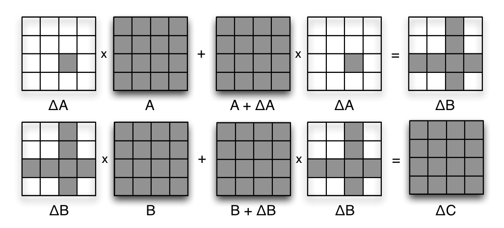
Figure 1: Evaluation of $\Delta{B}$ and $\Delta{C}$ for a single entry change in $A$. Gray entries have nonzero values.

The paper is organized as follows: Section 2 reviews the related work, Section 3 establishes the terminology and computational models used in the paper, Section 4 describes how to compute, represent, and propagate delta expressions, Section 5 analyzes the efficiency of incremental maintenance on common data analytics, Section 6 gives the system overview, and Section 7 experimentally validates our analysis.

2 Related Work

This section presents related work in different directions.

IVM and Stream Processing. Incremental View Maintenance techniques [7, 21, 17] support incremental updates of database materialized views by employing differential algorithms to re-evaluate the view expression. Chirkova et al. [10] present a detailed survey on this direction. Data stream processing engines [1, 27, 3] incrementally evaluate continuous queries as windows advance over unbounded input streams. In contrast to all the previous, this paper targets incremental maintenance of linear algebra programs as opposed to classical database (SQL) queries. The linear algebra domain has different semantics and primitives, thus the challenges and optimization techniques differ widely.

Iterative Computation.  Designing frameworks and computation models for iterative and incremental computation has received much attention lately. Differential dataflow [25] represents a new model of incremental computation for iterative algorithms, which relies on differences (deltas) being smaller and computationally cheaper than the inputs. This assumption does not hold for linear algebra programs because of the avalanche effect of input changes. Many systems optimize the MapReduce framework for iterative applications using techniques that cache and index loop-invariant data on local disks and persist materialized views between iterations [8, 15, 37]. More general systems support iterative computation and the DAG execution model, like Dryad [19] and Spark [35]; Mahout, MLbase [22] and others [12, 33, 26] provide scalable machine learning and data mining tools. All these systems are orthogonal to our work. This paper is concerned with the efficient re-evaluation of programs under incremental changes. Our framework, however, can be easily coupled with any of these underlying systems.

Scientific Databases.  There are also database systems specialized in array processing. RasDaMan [4] and AML [24] provide support for expressing and optimizing queries over multidimensional arrays, but are not geared towards scientific and numerical computing. ASAP [31] supports scientific computing primitives on a storage manager optimized for storing multidimensional arrays. RIOT [38] also provides an efficient out-of-core framework for scientific computing. However, none of these systems support incremental view maintenance for their workloads.

High Performance Computing.  The advent of numerical and scientific computing has fueled the demand for efficient matrix manipulation libraries. BLAS [14] provides low-level routines representing common linear algebra primitives to higher-level libraries, such as LINPACK, LAPACK, and ScaLAPACK for parallel processing. Hardware vendors such as Intel and AMD and code generators such as ATLAS [34] provide highly optimized BLAS implementations. In contrast, we focus on incremental maintenance of programs through efficient transformations and materialized views. The Linview compiler translates expensive BLAS routines to cheaper ones and thus further facilitates adoption of the optimized implementations.

PageRank.  There is a huge body of literature that is focused on PageRank, including the Markov chain model, solution methods, sensitivity and conditioning, and the updating problem. Surveys can be found in [23, 6]. The updating problem studies the effect of perturbations on the Markov chain and PageRank models, including sensitivity analysis, approximation, and exact evaluation methods. In principle, these methods are particularly tailored for these specific models. In contrast, this paper presents a novel model and framework for efficient incremental evaluation of general linear algebra programs through domain specific compiler translations and efficient code generation.

Incremental Statistical Frameworks.  Bayesian inference [5] uses Bayes’ rule to update the probability estimate for a hypothesis as additional evidence is acquired. These frameworks support a variety of applications such as pattern recognition and classification. Our work focuses on incrementalizing applications that can be expressed as linear algebra programs and generating efficient incremental programs for different runtime environments.

Programming Languages. The programming language community has extensively studied incremental computation and information flow [9]. It has developed languages and compilation techniques for translating high-level programs into executables that respond efficiently to dynamic changes. Self-adjusting computation targets incremental computation by exploiting dynamic dependency graphs and change propagation algorithms [2, 9]. These approaches: a) serve for general purpose programs as opposed to our domain specific approach, b) require serious programmer involvement by annotating modifiable portions of the program, and c) fail to efficiently capture the propagation of deltas among statements as presented in this paper.

3 Linear Algebra Programs

Linear algebra programs express computations using vectors and matrices as high-level abstractions. The language used to form such programs consists of the standard matrix manipulation primitives: matrix addition, subtraction, multiplication (including scalar, matrix-vector, and matrix-matrix multiplication), transpose, and inverse. A program expresses a computation as a sequence of statements, each consisting of an expression and a variable (matrix) storing its result. The program evaluates these expressions on a given dataset of input matrices and produces the result in one or more output matrices. The remaining matrices are auxiliary program matrices; they can be manipulated (materialized or removed) for performance reasons. For instance, the program of Example 1.1 consists of two statements evaluating the expressions over an input matrix $A$ and an auxiliary matrix $B$. The output matrix $C$ stores the computation result.

Computational complexity. In this paper, we refer to the cost of matrix multiplication as $\mathcal{O}(n^{\gamma})$ where $2\leq\gamma\leq 3$. In practice, the complexity of matrix multiplication, e.g., BLAS implementations [34], is bounded by cubic $\mathcal{O}(n^{3})$ time. Better algorithms with an exponent of $2.37+\epsilon$ are known (Coppersmith-Winograd and its successors); however, these algorithms are only relevant for astronomically large matrices. Our incremental techniques remain relevant as long as matrix multiplication stays asymptotically worse than quadratic time (a bound that has been conjectured to be achievable [11], but still seems far off). Note that the asymptotic lower bound for matrix multiplication is $\Omega(n^{2})$ operations because it needs to process at least $2n^{2}$ entries.

3.1 Iterative Programs

Many computational problems are iterative in nature. Iterative programs start from an approximate answer. Each iteration step improves the accuracy of the solution until the estimated error drops below a specified threshold. Iterative methods are often the only choice for problems for which direct solutions are either unknown (e.g., nonlinear equations) or prohibitively expensive to compute (e.g., due to large problem dimensions).

In this work we study (iterative) linear algebra programs from the viewpoint of incremental view maintenance (IVM). The execution of an iterative program generates a sequence of results, one for each iteration step. When the underlying data changes, IVM updates these results rather than re-evaluating them from scratch. We do so by propagating the delta expression of one iteration to subsequent iterations. With our incremental techniques, such delta expressions are cheaper to evaluate than the original expressions.

We consider iterative programs that execute a fixed number of iteration steps. The reason for this decision is that programs using convergence thresholds might yield a varying number of iteration steps after each update. Having different numbers of outcomes per update would require incremental maintenance to deal with outdated or missing old results; we leave this topic for future work. By fixing the number of iterations, we provide a fair comparison of the incremental and re-evaluation strategies.

3.2 Iterative Models

An iterative computation is governed by an iterative function that describes the computation at each step in terms of the results of previous iterations (materialized views) and a set of input matrices. Multiple iterative functions, or iterative models, might express the same computation but by using different numbers of iteration steps. For instance, the computation of the $k^{th}$ power of a matrix can be done in $k$ iterations or in $\log_{2}k$ iterations using the exponentiation by squaring method. Each iterative model of computation comes with its own complexity.

Our analysis of iterative programs considers three alternative models that require different numbers of iteration steps to compute the final result. These models allow us to explore trade-offs between computation time and memory consumption for both re-evaluation and incremental maintenance.

Linear Model. The linear iterative model evaluates the result of the current iteration based on the result of the previous iteration and a set of input matrices $\mathcal{I}$. It takes $k$ iteration steps to compute $T_{k}$.

$$T_{i}=\left\{\begin{array}[]{l@{~}l@{~}l}f(\mathcal{I})\hfil~{}&\hfil~{}&\mbox{for }\,i=1\\ g(T_{i-1},\mathcal{I})\hfil~{}&\hfil~{}&\mbox{for }\,i=2,3,\ldots\end{array}\right.$$

Example $A^{k}$: $T_{1}=A$ and $T_{i}=T_{i-1}\,A$ for $2\leq i\leq k$.

Exponential Model. In the exponential model, the result of the $i^{th}$ iteration depends on the result of the $(i/2)^{th}$ iteration. The model makes progressively larger steps between computed iterations, forming the sequence $T_{1}$, $T_{2}$, $T_{4}$, …. It takes $\mathcal{O}(\log{k})$ iteration steps to compute $T_{k}$.

$$T_{i}=\left\{\begin{array}[]{l@{~}l@{~}l}f(\mathcal{I})\hfil~{}&\hfil~{}&\mbox{for }\,i=1\\ g(T_{\nicefrac{{i}}{{2}}},\mathcal{I})\hfil~{}&\hfil~{}&\mbox{for }\,i=2,4,8\ldots\end{array}\right.$$

Example $A^{k}$: $T_{1}=A$ and $T_{i}=T_{\nicefrac{{i}}{{2}}}\,T_{\nicefrac{{i}}{{2}}}$ for $i=2,4,8,\ldots,k$.

Skip Model. Depending on the dimensions of input matrices, incremental evaluation using the above models might be suboptimal costwise. The skip-$s$ model represents a sweet spot between these two models. For a given skip size $s$, it relies on the exponential model to compute $T_{s}$ (generating the sequence $T_{2}$, $T_{4}$, …, $T_{s}$) and then generalizes the linear model to compute every $s^{th}$ iteration (generating the sequence $T_{2s}$, $T_{3s}$, …).

$$T_{i}=\left\{\begin{array}[]{l@{~}l@{~}l}f(\mathcal{I})\hfil~{}&\hfil~{}&\mbox{for }\,i=1\\ g(T_{i/2},\mathcal{I})\hfil~{}&\hfil~{}&\mbox{for }\,i=2,4,8,\ldots s\\ h(T_{i-s},T_{s},\mathcal{I})\hfil~{}&\hfil~{}&\mbox{for }\,i=2s,3s,\dots\end{array}\right.$$

Example $A^{k}$: For $s=8$, we have $T_{1}=A$, then $T_{i}=T_{\nicefrac{{i}}{{2}}}\,T_{\nicefrac{{i}}{{2}}}$ for $i=2,4,8$, and $T_{i}=T_{i-8}\,T_{8}$ for $i=16,24,32,\ldots,k$.

The skip model reconciles the two extremes: it corresponds to the linear model for $s=1$ and to the exponential model for $s=k$. In Section 5, we evaluate the time and space complexity of these models for a set of iterative programs.

4 Incremental Processing

In this section we develop techniques for converting linear algebra programs into functionally equivalent incremental programs suited for execution on dynamic datasets. An incremental program consists of a set of triggers, one trigger for each input matrix that might change over time. Each trigger has a list of update statements that maintain the result for updates to the associated input matrix. The total execution cost of an incremental program is the sum of execution costs of its triggers. Incremental programs incur lower computational complexity by converting the expensive operations of non-incremental programs to work with smaller datasets. Incremental programs combine precomputed results with low-rank updates to avoid costly operations, like matrix-matrix multiplications or matrix inversions.

Definition 4.1

A matrix $\mathcal{M}$ of dimensions $(n\times n)$ is said to have rank-$k$ if the maximum number of linearly independent rows or columns in the matrix is $k$. $\mathcal{M}$ is called a low-rank matrix if $k\ll n$.

4.1 Delta Derivation

The basic step in building incremental programs is the derivation of delta expressions $\Delta_{A}(E)$, which capture how the result of an expression $E$ changes as an input matrix $A$ is updated by $\Delta{A}$. We consider the update $\Delta{A}$, called a delta matrix, to be constant and independent of any other matrix. If we represent $E$ as a function of $A$, then $\Delta_{A}(E)=E(A+\Delta{A})-E(A)$. For presentation clarity, we omit the subscript in $\Delta_{A}(E)$ when $A$ is obvious from the context.

Most standard operations of linear algebra are amenable to incremental processing. Using the distributive and associative properties of common matrix operations, we derive the following set of delta rules for updates to $A$.

$$\Delta_{\text{A}}(E_{1}\,E_{2}):=\ (\Delta_{\text{A}}E_{1})\,E_{2}+E_{1}\,(\Delta_{\text{A}}E_{2})+\ (\Delta_{\text{A}}E_{1})(\Delta_{\text{A}}E_{2})$$

$$\Delta_{\text{A}}(E_{1}\pm E_{2}):= \ (\Delta_{\text{A}}E_{1})\pm(\Delta_{\text{A}}E_{2})$$

$$\Delta_{\text{A}}(\lambda\,E):= \ \lambda\,(\Delta_{\text{A}}E)$$

$$\Delta_{\text{A}}(E\,^{\text{T}}):= \ (\Delta_{\text{A}}E)^{\text{T}}$$

$$\Delta_{\text{A}}(E^{-1}):= \ (E+\Delta_{\text{A}}E)^{-1}-E^{-1}$$

$$\Delta_{\text{A}}(A):= \ \Delta{A}$$

$$\Delta_{\text{A}}(B):= \ 0\qquad(A\neq B)$$

We observe that the delta rule for matrix inversion references the original expression (twice), which implies that it is more expensive to compute the delta expression than the original expression. This claim is true for arbitrary updates to $A$ (e.g., random updates of all entries, all done at once). Later on, we discuss a special form of updates that admits efficient incremental maintenance of matrix inversions. Note that if $A$ does not appear in $E$, the delta expression for matrix inversion is zero.

Example 4.2

This example shows the derivation process. Consider the Ordinary Least Squares method for estimating the unknown parameters in a linear regression model. We want to find a statistical estimate of the parameter $\beta^{*}$ best satisfying $Y=X\beta$. The solution, written as a linear algebra program, is $\beta^{*}=(X^{\text{T}}\,X)^{-1}\,X^{\text{T}}\,Y$. Here, we focus on how to derive the delta expression for $\beta^{*}$ under updates to $X$. We defer an in-depth cost analysis of the method to Section 5. Let $Z=X^{\text{T}}\,X$ and $W=Z^{-1}$. Then

$$\Delta{Z} =\Delta(X^{\text{T}}\,X)$$

$$=(\Delta{(X^{\text{T}})})\,X+X^{\text{T}}\,(\Delta{(X)})+(\Delta{(X^{\text{T}})})\,(\Delta{(X)})$$

$$=(\Delta{X})^{\text{T}}\,X+X^{\text{T}}\,(\Delta{X})+(\Delta{X})^{\text{T}}\,(\Delta{X})$$

$$\Delta{W} =(Z+\Delta{Z})^{-1}-Z^{-1}$$

$$\Delta{\beta^{*}} =(\Delta{W})\,X^{\text{T}}\,Y+W\,(\Delta{X})^{\text{T}}\,Y+(\Delta{W})\,(\Delta{X})^{\text{T}}\,Y \Box$$

For random matrix updates, incrementally computing a matrix inverse is prohibitively expensive. The Sherman-Morrison formula [29] provides a numerically cheap way of maintaining the inverse of an invertible matrix for rank-$1$ updates. Given a rank-$1$ update $u\,v^{\text{T}}$, where $u$ and $v$ are column vectors, if $E$ and $E+u\,v^{\text{T}}$ are nonsingular, then

$$\Delta{(E^{-1})}:=-\frac{E^{-1}\,u\,v^{\text{T}}\,E^{-1}}{1+v^{\text{T}}\,E^{-1}\,u}$$

Note that $\Delta{(E^{-1})}$ is also a rank-$1$ matrix. For instance, $\Delta{(E^{-1})}=p\,q^{\text{T}}$, where $p=\lambda\,E^{-1}u$ and $q=(E^{-1})^{\text{T}}\,v$ are column vectors, and $\lambda$ is a scalar (observe that the denominator is a scalar too). Thus, incrementally computing $E^{-1}$ for rank-$1$ updates to $E$ requires $\mathcal{O}(n^{2})$ operations; it avoids any matrix-matrix multiplication and inversion operations.

Example 4.3

We apply the Sherman-Morrison formula to Example 4.2. We start by considering rank-$1$ updates to $X$. Let $\Delta{X}=u\,v^{\text{T}}$, then

$$\Delta{Z}= v\,u^{\text{T}}\,X+X^{\text{T}}\,u\,v^{\text{T}}+v\,u^{\text{T}}\,u\,v^{\text{T}}$$

$$= v\,(u^{\text{T}}\,X)+(X^{\text{T}}\,u+v\,u^{\text{T}}\,u)\,v^{\text{T}}$$

The parentheses denote the subexpressions that evaluate to vectors. We observe that each of the monomials is a vector outer product. Thus, we can write $\Delta{Z}=\Delta{Z_{1}}+\Delta{Z_{2}}$, where $\Delta{Z_{1}}=p_{1}\,q_{1}^{\text{T}}$ and $\Delta{Z_{2}}=p_{2}\,q_{2}^{\text{T}}$. Now we can apply the formula on each outer product in turn.

$$\Delta_{Z_{1}}{(W)}= -\frac{W\,p_{1}\,q_{1}^{\text{T}}\,W}{1+q_{1}^{\text{T}}\,W\,p_{1}}$$

$$\Delta_{Z_{2}}{(W)}= -\frac{(W+\Delta_{Z_{1}}(W))\,p_{2}\,q_{2}^{\text{T}}\,(W+\Delta_{Z_{1}}(W))}{1+q_{2}^{\text{T}}\,(W+\Delta_{Z_{1}}(W))\,p_{2}}$$

Finally, $\Delta_{Z}{(W)}=\Delta_{Z_{1}}{(W)}+\Delta_{Z_{2}}{(W)}$. The evaluation cost of $\Delta_{Z}{(W)}$ is $\mathcal{O}(n^{2})$ operations, as discussed above. For comparison, the evaluation cost of $\Delta{W}$ in Example 4.2 is $\mathcal{O}(n^{\gamma})$ operations. $\Box$

In the above OLS examples, $\Delta{W}$ is a matrix with potentially all nonzero entries. If we store these entries in a single delta matrix, we still need to perform $\mathcal{O}(n^{\gamma})$-cost matrix multiplications in order to compute $\Delta{\beta^{*}}$. Next, we propose an alternative way of representing delta expressions that allows us to stay in the realm of $\mathcal{O}(n^{2})$ computations.

4.2 Delta Representation

In this section we discuss how to represent delta expressions in a form that is amenable to incremental processing. This form also dictates the structure of admissible updates to input matrices. Incremental processing brings no benefit if the whole input matrix changes arbitrarily at once.

Let us consider updates of the smallest granularity – single entry changes of an input matrix. The delta matrix capturing such an update contains exactly one nonzero entry being updated. The following example shows that even a minor change, when propagated naïvely, can cause incremental processing to be more expensive than recomputation.

Example 4.4

Consider the program of Example 1.1 for computing the fourth power of a given matrix $A$. Following the delta rules we write $\Delta{B}=(\Delta{A})\,A+(A+\Delta{A})\,(\Delta{A})$. Fig. 1 shows the effect of a single entry change in $A$ on $\Delta{B}$. The single entry change has escalated to a change of one row and one column in $B$. When we propagate this change to the next statement, $\Delta{C}$ becomes a fully-perturbed delta matrix, that is, all entries might have nonzero values.

Now suppose we want to evaluate $A^{8}$, so we extend the program with the statement $D:=C\,C$. To evaluate $\Delta{D}$, which is expressed similarly as $\Delta{B}$, we need to perform two matrix-matrix multiplications and two matrix additions. Clearly, in this case, it is more efficient to recompute $D$ using the new $C$ than to incrementally maintain it with $\Delta{D}$.$\Box$

The above example shows that linear algebra programs are, in general, sensitive to input changes. Even a single entry change in the input can cause an avalanche effect of perturbations, quickly escalating to its extreme after executing merely two statements.

We propose a novel approach to deal with escalating updates. So far, we have used a single matrix to store the result of a delta expression. We observe that such representation is highly redundant as delta matrices typically have low ranks. Although a delta matrix might contain all nonzero entries, the number of linearly independent rows or columns is relatively small compared to the matrix size. In Example 4.4, $\Delta{B}$ has a rank of at most two.

We maintain a delta matrix in a factored form, represented as a product of two low-rank matrices. The factored form enables more efficient evaluation of subsequent delta expressions. Due to the associativity and distributivity of matrix multiplication, we can base the evaluation strategy for delta expressions solely on matrix-vector products, and thus avoid expensive matrix-matrix multiplications.

To achieve this goal, we also represent updates of input matrices in the factored form. In this paper we consider rank-$k$ changes of input matrices as they can capture many practical update patterns. For instance, the simplest rank-$1$ updates can express perturbations of one complete row or column in a matrix, or even changes of the whole matrix when the same vector is added to every row or column.

In Example 4.4, consider a rank-$1$ update $\Delta{A}=u_{\text{A}}v_{\text{A}}^{\text{T}}$, where $u_{\text{A}}$ and $v_{\text{A}}$ are column vectors, then $\Delta{B}=u_{\text{A}}\,(v_{\text{A}}^{\text{T}}\,A)+(A\,u_{\text{A}})\,v_{\text{A}}^{\text{T}}+(u_{\text{A}}\,v_{\text{A}}^{\text{T}}\,u_{\text{A}})\,v_{\text{A}}^{\text{T}}$ is a sum of three outer products. The parentheses denote the factored subexpressions (vectors). The evaluation order enforced by these parentheses yields only matrix-vector and vector-vector multiplications. Thus, the evaluation of $\Delta{B}$ requires only $\mathcal{O}(n^{2})$ operations.

Instead of representing delta expressions as sums of outer products, we maintain them in a more compact vectorized form for performance and presentation reasons. A sum of $k$ outer products is equivalent to a single product of two matrices of sizes $(n\times k)$ and $(k\times n)$, which are obtained by stacking the corresponding vectors together. For instance,

$$u_{1}\,v_{1}^{\text{T}}+u_{2}\,v_{2}^{\text{T}}+u_{3}\,v_{3}^{\text{T}}=\begin{bmatrix}u_{1}&u_{2}&u_{3}\end{bmatrix}\,\begin{bmatrix}v_{1}^{\text{T}}\\ v_{2}^{\text{T}}\\ v_{3}^{\text{T}}\\ \end{bmatrix}=P\,Q^{\text{T}}$$

where $P$ and $Q$ are $(n\times 3)$ block matrices.

To summarize, we maintain a delta expression as a product of two low-rank matrices with dimensions $(n\times k)$ and $(k\times n)$, where $k\ll n$. This representation allows efficient evaluation of subsequent delta expressions without involving expensive $\mathcal{O}(n^{\gamma})$ operations; instead, we perform only $\mathcal{O}(kn^{2})$ operations. A similar analysis naturally follows for rank-$k$ updates with linearly increasing evaluation costs; the benefit of incremental processing diminishes as $k$ approaches the dominant matrix dimension.

Considering low-rank updates of matrices also opens opportunities to benefit from previous work on incrementalizing complex linear algebra operations. We have already discussed the Sherman-Morrison method of incrementally computing the inverse of a matrix for rank-$1$ updates. Other work [13, 30] investigates rank-$1$ updates in different matrix factorizations, like SVD and Cholesky decomposition. We can further use these new primitives to enrich our language, and, consequently, support more sophisticated programs.

4.3 Delta Propagation

When constructing incremental programs we propagate delta expressions from one statement to another. For delta expressions with multiple monomials, factored representations include increasingly more outer products. That raises the cost of evaluating these expressions. In Example 4.4, $\Delta{B}$ consists of three outer products compacted as

$$\Delta{B}=\begin{bmatrix}u_{\text{A}}&(A\,u_{\text{A}})&(u_{\text{A}}\,(v_{\text{A}}^{\text{T}}\,u_{\text{A}}))\end{bmatrix}\,\begin{bmatrix}v_{\text{A}}^{\text{T}}\,A\\ v_{\text{A}}^{\text{T}}\\ v_{\text{A}}^{\text{T}}\end{bmatrix}=U_{\text{B}}\,V_{\text{B}}^{\text{T}}$$

Here, $U_{\text{B}}$ and $V_{\text{B}}$ are $(n\times 3)$ block matrices. Akin to $\Delta{B}$, $\Delta{C}$ is also a sum of three products expressed using $B$, $U_{\text{B}}$, and $V_{\text{B}}$, and compacted as a product of two $(n\times 9)$ block matrices. Finally, we use $C$ and the factored form of $\Delta{C}$ to express $\Delta{D}$ as a product of two $(n\times 27)$ block matrices.

Observe that $U_{\text{B}}$ and $V_{\text{B}}$ have linearly dependent columns, which suggests that we could have an even more compact representation of these matrices. A less redundant form, which reduces the size of $U_{\text{B}}$ and $V_{\text{B}}$, guarantees less work in evaluating subsequent delta expressions. To alleviate the redundancy in representation, we reduce the number of monomials in a delta expression by extracting common factors among them. This syntactic approach does not guarantee the most compact representation of a delta expression, which is determined by the rank of the delta matrix. However, computing the exact rank of the delta matrix requires inspection of the matrix values, which we deem too expensive. The factored form of $\Delta{B}$ of Example 4.4 is

$$\Delta{B}=\begin{bmatrix}u_{\text{A}}&(A\,u_{\text{A}}+u_{\text{A}}\,(v_{\text{A}}^{\text{T}}\,u_{\text{A}}))\end{bmatrix}\,\begin{bmatrix}v_{\text{A}}^{\text{T}}\,A\\ v_{\text{A}}^{\text{T}}\end{bmatrix}=U_{\text{B}}\,V_{\text{B}}^{\text{T}}$$

Here, $U_{\text{B}}$ and $V_{\text{B}}$ are $(n\times 2)$ matrices. $\Delta{C}$ is a product of two $(n\times 4)$ matrices and $\Delta{D}$ multiplies two $(n\times 8)$ matrices.

4.4 Putting It All Together

So far we have discussed how to derive, represent, and propagate delta expressions. In this section we put these techniques together into an algorithm that compiles a given program to its incremental version.

Alg. 1 shows the algorithm that transforms a program $\mathcal{P}$ into a set of trigger functions $\mathcal{T}$, each of them handling updates to one input matrix. For updates arriving as vector outer products, the matching trigger incrementally maintains the computation result by evaluating a sequence of assignment statements ($:=$) and update statements ($\mathrel{+}=$).

Algorithm 1 Compile program $\mathcal{P}$ into a set of triggers $\mathcal{T}$

1:function Compile($\mathcal{P}$, $\mathcal{I}$)

2:    $\mathcal{T}\leftarrow\emptyset$

3:    for each $X\in\mathcal{I}$ do

4:       $\mathcal{D}\leftarrow\mbox{list}(\langle X,u,v\rangle)$

5:       for each $\langle A_{i},E_{i}\rangle\in\mathcal{P}$ do

6:          $\langle P_{i},Q_{i}\rangle\leftarrow\textsc{ComputeDelta}(E_{i},\mathcal{D})$

7:          $\mathcal{D}\leftarrow\mathcal{D}.\mbox{append}(\langle A_{i},P_{i},Q_{i}\rangle)$        

8:       $\mathcal{T}\leftarrow\mathcal{T}\ \cup\,\textsc{BuildTrigger}(X,\mathcal{D})$     

9:    return $\mathcal{T}$

The algorithm takes as input two parameters: (1) a program $\mathcal{P}$ expressed as a list of assignment statements, where each statement is defined as a tuple $\langle A_{i},E_{i}\rangle$ of an expression $E_{i}$ and a matrix $A_{i}$ storing the result, and (2) a set of input matrices $\mathcal{I}$, and outputs a set of trigger functions $\mathcal{T}$.

The ComputeDelta function follows the rules from Section 4.1 to derive the delta for a given expression $E_{i}$ and an update to $X$. The function returns two expressions that together form the delta, $\Delta{A_{i}}=P_{i}\,Q_{i}^{\text{T}}$. As discussed in Section 4.2, $P_{i}$ and $Q_{i}$ are block matrices in which each block has its defining expression.

The algorithm maintains a list of the generated delta expressions in $\mathcal{D}$. Each entry in $\mathcal{D}$ corresponds to one update statement of the trigger program. The entries respect the order of statements in the original program.

Note that ComputeDelta takes $\mathcal{D}$ as input. The list of matrices affected by a change in $X$ – initially containing only $X$ – expands throughout the execution of the algorithm. One expression might reference more than one such matrix, so we have to deal with multiple matrix updates to derive the correct delta expression. The delta rules presented in Section 4.1 consider only single matrix updates, but we can easily extend them to handle multiple matrix updates. Suppose $\mathcal{D}=\{A,B,\ldots\}$ is a set of the affected matrices that also appear in an expression $E$. Then, $\Delta_{\mathcal{D}}(E):=\Delta_{A}(E)+\Delta_{(\mathcal{D}\setminus\{A\})}(E+\Delta_{A}(E))$. The delta rule considers each matrix update in turn. The order of applying the matrix updates is irrelevant.

Example 4.5

Consider the expression $E=A\,B$ and the updates $\Delta{A}$ and $\Delta{B}$. Then,

$$\Delta_{\{A,B\}}{(E)}= \Delta_{A}(E)+\Delta_{B}(E+\Delta_{A}(E))$$

$$= (\Delta{A})\,B+\Delta_{B}(A\,B+(\Delta{A})\,B)$$

$$= (\Delta{A})\,B+A\,(\Delta{B})+(\Delta{A})\,(\Delta{B}) \Box$$

The BuildTrigger function converts the derived deltas $\mathcal{D}$ for updates to $X$ into a trigger program. The function first generates the assignment statements that evaluate $P_{i}$ and $Q_{i}$ for each delta expression, and then the update statements for each of the affected matrices.

Example 4.6

Consider the program that computes the fourth power of a given matrix A, discussed in Example 1.1 and Example 4.4. Algorithm 1 compiles the program and produces the following trigger for updates to $A$.

ON UPDATE A BY (u_A,v_A):    U_B := [ u_A   (A u_A + u_A (v_A^​T u_A)) ];    V_B := [ (A^T v_A)   v_A ];    U_C := [ U_B   (B U_B + U_B (V_B^​T U_B)) ];    V_C := [ (B^T V_B)   V_B ];    A += u_A v_A^​T;   B += U_B V_B^​T;   C += U_C V_C^​T;Here, $u_{\text{A}}$ and $v_{\text{A}}$ are column vectors, $U_{B}$, $V_{B}$, $U_{C}$, and $V_{C}$ are block matrices. Each delta, including the input change, is a product of two low-rank matrices. $\Box$

Model	Matrix Powers	Sums of Matrix Powers	General form: $T_{i+1}=A\,T_{i}+B$
Linear	$P_{i}=\left\{\begin{array}[]{l}A\\ A\,P_{i-1}\end{array}\right.$	$S_{i}=\left\{\begin{array}[]{l}I\\ A\,S_{i-1}+I\end{array}\right.$	$T_{i}=\left\{\begin{array}[]{l}A\,T_{0}+B\\ A\,T_{i-1}+B\end{array}\right.$	$\begin{array}[]{l@{~}l}\hfil~{}&\mbox{for }\,i=1\\ \hfil~{}&\mbox{for }\,i=2,3,\ldots,k\end{array}$
Exponential	$P_{i}=\left\{\begin{array}[]{l}A\\ P_{i/2}\,P_{i/2}\end{array}\right.$	$S_{i}=\left\{\begin{array}[]{l}I\\ P_{i/2}\,S_{i/2}+S_{i/2}\end{array}\right.$	$T_{i}=\left\{\begin{array}[]{l}A\,T_{0}+B\\ P_{i/2}\,T_{i/2}+S_{i/2}\,B\end{array}\right.$	$\begin{array}[]{l@{~}l}\hfil~{}&\mbox{for }\,i=1\\ \hfil~{}&\mbox{for }\,i=2,4,8,\ldots,k\end{array}$
Skip-$s$	$P_{i}=\left\{\begin{array}[]{l}A\\ P_{i/2}\,P_{i/2}\\ P_{s}\,P_{i-s}\end{array}\right.$	$S_{i}=\left\{\begin{array}[]{l}I\\ P_{i/2}\,S_{i/2}+S_{i/2}\\ P_{s}\,S_{i-s}+S_{s}\end{array}\right.$	$T_{i}=\left\{\begin{array}[]{l}A\,T_{0}+B\\ P_{i/2}\,T_{i/2}+S_{i/2}\,B\\ P_{s}\,T_{i-s}+S_{s}\,B\end{array}\right.$	$\begin{array}[]{l@{~}l@{~}l}\hfil~{}&\mbox{for }i=1\hfil~{}\\ \hfil~{}&\mbox{for }i=2,4,8,\ldots,s\hfil~{}\\ \hfil~{}&\mbox{for }i=2s,3s,\ldots,k\hfil~{}\end{array}$

Table 1: The computation of matrix powers, sums of matrix powers, and the general iterative computation expressed as recurrence relations. For simplicity of the presentation, we assume that $\log_{2}k$, $\log_{2}s$, and $\frac{k}{s}$ are integers.

5 Incremental Analytics

In this section we analyze a set of programs that have wide application across many domains from the perspective of incremental maintenance. We study the time and space complexity of both re-evaluation and incremental evaluation over dynamic datasets. We show analytically that, in most of these examples, incremental maintenance exhibits better asymptotic behavior than re-evaluation in terms of execution time. In other cases, a combination of the two strategies offers the lowest time complexity. Note that our incremental techniques are general and apply to a broader range of linear algebra programs than those presented here.

5.1 Ordinary Least Squares

Ordinary Least Squares (OLS) is a classical method for fitting a curve to data. The method finds a statistical estimate of the parameter $\beta^{*}$ best satisfying $Y=X\beta$. Here, $X=(m\times n)$ is a set of predictors, and $Y=(m\times p)$ is a set of responses that we wish to model via a function of $X$ with parameters $\beta$. The best statistical estimate is $\beta^{*}=(X^{T}X)^{-1}X^{T}Y$. Data practitioners often build regression models from incomplete or inaccurate data to gain preliminary insights about the data or to test their hypotheses. As new data points arrive or measurements become more accurate, incremental maintenance avoids expensive reconstruction of the whole model, saving time and frustration.

First, consider the cost of incrementally computing the matrix inverse for changes in $X$. Let $Z=X^{\text{T}}\,X$, $W=Z^{-1}$, and $\Delta{X}=u\,v^{\text{T}}$. As derived in Example 4.2,

$$\Delta{Z}=\begin{bmatrix}v&(X^{\text{T}}\,u+v\,u^{\text{T}}\,u)\end{bmatrix}\,\begin{bmatrix}u^{\text{T}}\,X\\ v^{\text{T}}\\ \end{bmatrix}=\begin{bmatrix}p_{1}&p_{2}\end{bmatrix}\,\begin{bmatrix}q_{1}^{\text{T}}\\ q_{2}^{\text{T}}\\ \end{bmatrix}$$

The cost of computing $p_{2}$ and $q_{1}$ is $\mathcal{O}(mn)$. The vectors $p_{1}$, $q_{1}$, $p_{2}$, and $q_{2}$ have size $(n\times 1)$.

As shown in Example 4.3, we could represent the delta expressions of $W$ as a sum of two outer products, $\Delta_{Z_{1}}(W)=r_{1}\,s_{1}^{\text{T}}$ and $\Delta_{Z_{2}}(W)=r_{2}\,s_{2}^{\text{T}}$; for instance, $s_{1}=W^{\text{T}}\,q_{1}$ and $r_{1}$ is the remaining subexpression in $\Delta_{Z_{1}}(W)$.

The computation of $r_{1}$, $q_{1}$, $r_{2}$, and $q_{2}$ involves only matrix-vector $\mathcal{O}(n^{2})$ operations. Then the overall cost of incremental maintenance of $W$ is $\mathcal{O}(n^{2}+mn)$. For comparison, re-evaluation of $W$ takes $\mathcal{O}(n^{\gamma}+mn^{2})$ operations.

Finally, we compute $\Delta{\beta^{*}}$ for updates $\Delta{X}=u\,v^{\text{T}}$ and $\Delta{W}=R\,S^{\text{T}}$, where $R=\begin{bmatrix}r_{1}&r_{2}\end{bmatrix}$ and $S=\begin{bmatrix}s_{1}&s_{2}\end{bmatrix}$ are $(n\times 2)$ block matrices and $\Delta{\beta^{*}}=R\,S^{\text{T}}\,X^{\text{T}}\,Y+W\,v\,u^{\text{T}}\,Y+R\,S^{\text{T}}\,v\,u^{\text{T}}\,Y$. The optimum evaluation order for this expression depends on the size of $X$ and $Y$. In general, the cost of incremental maintenance of $\beta^{*}$ is $\mathcal{O}(n^{2}+mp+np+mn)$. For comparison, re-evaluation of $\beta^{*}$ takes $\mathcal{O}(mnp+n^{2}\min{(m,p)})$ operations.

Overall, considering both phases, the incremental maintenance of $\beta{{}^{*}}$ for updates to $X$ has lower computation complexity than re-evaluation. This holds even when $Y$ is of small dimension (e.g., vector); the matrix inversion cost still dominates in the re-evaluation method. The space complexity of both strategies is $\mathcal{O}(n^{2})$.

	Model	(Sums of) Matrix Powers			General form: $T_{i+1}=A\,T_{i}+B$
		Re-evaluation	Incremental		Re-evaluation	Incremental	Hybrid
Time	Linear	$n^{\gamma}k$	$n^{2}k^{2}$		$pn^{2}k$	$(n^{2}+pn)k^{2}$	$pn^{2}k$
	Exponential	$n^{\gamma}\log{k}$	$n^{2}k$		$(n^{\gamma}+pn^{2})\log{k}$	$(n^{2}+pn)k$	$pn^{2}\log{k}+n^{2}k$
	Skip-$s$	$n^{\gamma}(\log{s}+\frac{k}{s})$	$n^{2}\frac{k^{2}}{s}$		$n^{\gamma}\log{s}+pn^{2}(\log{s}+\frac{k}{s})$	$(n^{2}+np)\frac{k^{2}}{s}$	$pn^{2}(\log{s}+\frac{k}{s})+n^{2}s$
Space	Linear	$n^{2}$	$n^{2}k$		$n^{2}+np$	$n^{2}+knp$	$n^{2}+knp$
	Exponential	$n^{2}$	$n^{2}\log{k}$		$n^{2}+np$	$(n^{2}+np)\log{k}$	$(n^{2}+np)\log{k}$
	Skip-$s$	$n^{2}$	$n^{2}(\log{s}+\frac{k}{s})$		$n^{2}+np$	$(n^{2}+np)\log{s}+np\frac{k}{s}$	$(n^{2}+np)\log{s}+np\frac{k}{s}$

Table 2: The time and space complexity (expressed in big-O notation) of the different evaluation techniques for the various computational models under rank-$1$ updates to matrix $A$ where $2\leq\gamma\leq 3$ as described in Section 3.

5.2 Matrix Powers

Our next analysis includes the computation of $A^{k}$ of a square matrix $A$ for some fixed $k>0$. Matrix powers play an important role in many different domains including computing the stochastic matrix of a Markov chain after $k$ steps, solving systems of linear differential equations using matrix exponentials, answering graph reachability queries where $k$ represents the maximum path length, and computing PageRank using the power method.

Matrix powers also provide the basis for the incremental analysis of programs having more general forms of iterative computation. In such programs we often decide to evaluate several iteration steps at once for performance reasons, and matrix powers allow us to express these compound transformations between iterations, as shown later on.

5.2.1 Iterative Models

Table 1 expresses the matrix power computation using the iterative models presented in Section 3. In all cases, $A$ is an input matrix that changes over time, and $P_{k}$ contains the final result $A^{k}$. The linear model computes the result of every iteration, while the exponential model makes progressively larger leaps between consecutive iterations evaluating only $\log_{2}{k}$ results. The skip model precomputes $A^{s}$ in $P_{s}$ using the exponential model and then reuses $P_{s}$ to compute every $s^{th}$ subsequent iteration.

Expressing the matrix power computation as an iterative process eases the complexity analysis of both re-evaluation and incremental maintenance, which we show next.

5.2.2 Cost Analysis

We analyze the time and space complexity of re-evaluation and incremental maintenance of $P_{k}$ for rank-$1$ updates to $A$, denoted by $\Delta{A}=u\,v^{\text{T}}$. We assume that $A$ is a dense square matrix of size $(n\times n)$.

Re-evaluation. Table 2 shows the time complexity of re-evaluating $P_{k}$ in different iterative models. The re-evaluation strategy first updates $A$ by $\Delta{A}$ and then recomputes $P_{k}$ using the new value of $A$. All three models perform one $\mathcal{O}(n^{\gamma})$ matrix-matrix multiplication per iteration. The total execution cost thus depends on the number of iteration steps: The exponential method clearly requires the fewest iterations $\log_{2}{k}$, followed by $(\log_{2}s+\frac{k}{s})$ and $k$ iterations of the skip and linear models.

Table 2 also shows the space complexity of re-evaluation in the three iterative models. The memory consumption of these models is independent of the number of iterations. At each iteration step these models use at most two previously computed values, but not the full history of $P_{i}$ values.

Incremental Maintenance. This strategy captures the change in the result of every iteration as a product of two low-rank matrices $\Delta{P_{i}}=U_{i}\,V_{i}^{\text{T}}$. The size of $U_{i}$ and $V_{i}$ and, in general, the rank of $\Delta{P_{i}}$ grow linearly with every iteration step. We consider the case when $k\ll n$ in which we can profit from the low-rank delta representation. This is a realistic assumption as many practical computations consider large matrices and relatively few iterations; for example, 80.7% of the pages in a PageRank computation converge in less than 15 iterations [20].

Table 2 shows the time complexity of incremental maintenance of $P_{k}$ in the three iterative models. Incremental maintenance exhibits better asymptotic behavior than re-evaluation in all three models, with the exponential model clearly dominating the others. Appendix A presents a detailed cost analysis.

The performance improvement comes at the cost of increased memory consumption, as incremental maintenance requires storing the result of every iteration step. Table 2 also shows the space complexity of incremental maintenance for the three iterative models.

5.2.3 Sums of Matrix Powers

A form of matrix powers that frequently occurs in iterative computations is a sum of matrix powers. The goal is to compute $S_{k}=I+A+\ldots A^{k-2}+A^{k-1}$, for a given matrix $A$ and fixed $k>0$. Here, $I$ is the identity matrix.

In Table 1 we express this computation using the iterative models discussed earlier. In the exponential and skip models, the computation of $S_{k}$ relies on the results of matrix power computation, denoted by $P_{i}$ and evaluated using the exponential model discussed earlier.

For all three models, the time and space complexity of computing sums of matrix powers is the same in terms of big-O notation as that of computing matrix powers. The intuition behind this result is that the complexity of each iteration step has remained unchanged. Each iteration step performs one matrix addition more, but the execution cost is still dominated by the matrix multiplication. We omit the detailed analysis due to space constraints.

5.3 General Form: T_i+1 = AT_i + B

The two examples of matrix power computation provide the basis for the discussion about a more general form of iterative computation: $T_{i+1}=A\,T_{i}+B$, where $A$ and $B$ are input matrices. In contrast to the previous analysis of matrix powers, this iterative computation involves also non-square matrices, $T=(n\times p)$, $A=(n\times n)$, and $B=(n\times p)$, making the choice of the optimum evaluation strategy dependent on the values of $n$, $p$, $k$, and $s$.

Many iterative algorithms share this form of computation including gradient descent, PageRank, iterative methods for solving systems of linear equations, and the power iteration method for eigenvalue computation. Here, we analyze the complexity of the general form of iterative computation, and the same conclusions hold in all these cases.

5.3.1 Iterative Models

The iterative models of the form $T_{i+1}=A\,T_{i}+B$, which are presented in Table 1, rely on the computations of matrix powers and sums of matrix powers. To understand the relationship between these computations, consider the iterative process $T_{i+1}=A\,T_{i}+B$ that has been “unrolled” for $k$ iteration steps. The direct formula for computing $T_{i+k}$ from $T_{i}$ is $T_{i+k}=A^{k}\,T_{i}+(A^{k-1}+\ldots+A+I)\,B$.

We observe that $A^{k}$ and $\sum_{i=0}^{k-1}{A^{i}}$ correspond to $P_{k}$ and $S_{k}$ in the earlier examples, for which we have already shown efficient (incremental) evaluation strategies. Thus, to compute $T_{i}$, we maintain two auxiliary views $P_{i}$ and $S_{i}$ evaluating matrix powers and sums of matrix powers using the exponential model discussed before.

5.3.2 Cost Analysis

We analyze the time and space complexity of re-evaluation and incremental maintenance of $T_{k}$ for rank-$1$ updates to $A$, denoted by $\Delta{A}=u\,v^{\text{T}}$. We assume that $A$ is an $(n\times n)$ dense matrix and that $T_{i}$ and $B$ are $(n\times p)$ matrices. We omit a similar analysis for changes in $B$ due to space constraints.

We also analyze a combination of the two strategies, called hybrid evaluation, which avoids the factorization of delta expressions but instead represents them as single matrices. We consider this strategy because the size $(n\times p)$ of the delta matrix $\Delta{T_{i}}$ might be insufficient to justify the use of the factored form. For instance, consider an extreme case when $T_{i}$ is a column vector ($p=1$), then $\Delta{T_{i}}$ has rank $1$, and further decomposition into a product of two matrices would just increase the evaluation cost. In such cases, hybrid evaluation expresses $\Delta{T_{i}}$ as a single matrix and propagates it to the subsequent iterations.

Table 2 presents the time complexity of re-evaluation, incremental and hybrid evaluation of the $T_{i+1}=A\,T_{i}+B$ computation expressed in different iterative models for rank-$1$ updates to $A$. The same complexity results hold for the special form of iterative computation where $B=0$. We discuss the results for each evaluation strategy next. Appendix B shows a detailed cost analysis.

Table 2 also shows the space complexity of the three iterative models when executed using different evaluation strategies. The re-evaluation strategy maintains the result of $T_{i}$, and if needed $P_{i}$ and $S_{i}$, only for the current iteration; it also stores the input matrices $A$ and $B$. In contrast, the incremental and hybrid evaluation strategies materialize the result of every iteration, thus the memory consumption depends on the number of performed iterations.

Re-evaluation. The choice of the iterative model with the best asymptotic behavior depends on the value of parameters $n$, $p$, $k$, and $s$. The time complexities from Table 2 shows that the linear model incurs the lowest time complexity when $p\ll n$, otherwise the exponential model dominates the others in terms of the running time. We analyze the cost of each iterative model next. Note that the re-evaluation strategy first updates $A$ by $\Delta{A}$ and then recomputes $T_{i}$, and if needed $P_{i}$ and $S_{i}$, using the new value of $A$.

$\bullet$ Linear model. The computation performs $k$ iterations, where each one incurs the cost of $\mathcal{O}(pn^{2})$, and thus the total cost is $\mathcal{O}(pn^{2}k)$.

$\bullet$ Exponential model. Maintaining $P_{i}$ and $S_{i}$ takes $\mathcal{O}(n^{\gamma})$ operations as discussed before, while recomputing $T_{i}$ requires $\mathcal{O}(pn^{2})$ operations. Overall, the re-evaluation cost is $\mathcal{O}((n^{\gamma}+pn^{2})log{k})$.

$\bullet$ Skip model. The skip model combines the above two models. Maintaining $P_{s}$ and $S_{s}$ takes $\mathcal{O}(n^{\gamma}\log{s})$ operations as shown earlier, while recomputing $T_{i}$ costs $\mathcal{O}(pn^{2})$ per iteration. The total number of $(\log_{2}{s}+\frac{k}{s})$ iterations yields the total cost of $\mathcal{O}(n^{\gamma}\log{s}+pn^{2}(\log{s}+\frac{k}{s}))$.

Incremental Maintenance. Table 2 shows that incremental evaluation of $T_{k}$ using the exponential model incurs the lowest time complexity among the three iterative models. It also outperforms complete re-evaluation when $p>n$, but the performance benefit diminishes as $p$ becomes smaller than $n$. For the extreme case when $p=1$, complete re-evaluation and incremental maintenance have the same asymptotic behavior, but in practice re-evaluation performs fewer operations as it avoids the overhead of computing and propagating the factored deltas. We show next how to combine the best of both worlds to lower the execution time when $p\ll n$.

Hybrid evaluation. Hybrid evaluation departs from incremental maintenance in that it represents the change in the result of every iteration as a single matrix instead of an outer product of two vectors. The benefit of hybrid evaluation arises when the rank of $\Delta{T_{i}}=(n\times p)$ is not large enough to justify the use of the factored form; that is, when the dimension $p$ or $n$ is comparable with $k$.

Table 2 shows the time complexity of hybrid evaluation of the $T_{i+1}=A\,T_{i}+B$ computation expressed in different iterative models for rank-$1$ updates to $A$. For the extreme case when $p=1$, the skip model performs $\mathcal{O}(\log{s}+\frac{k}{s}+s)$ matrix-vector multiplications. In comparison, re-evaluation and incremental maintenance perform $\mathcal{O}(k)$ such operations. Thus, the skip model of hybrid evaluation bears the promise of better performance for the given values of $k$ and $s$.

6 System Overview

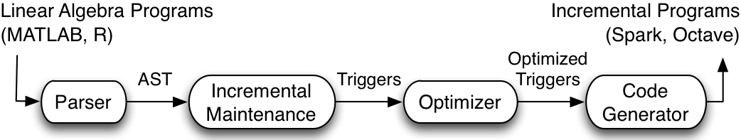
Figure 2: The Linview system overview

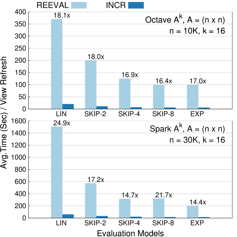
(a) Matrix Powers

(b) Scalability of Powers $(n)$

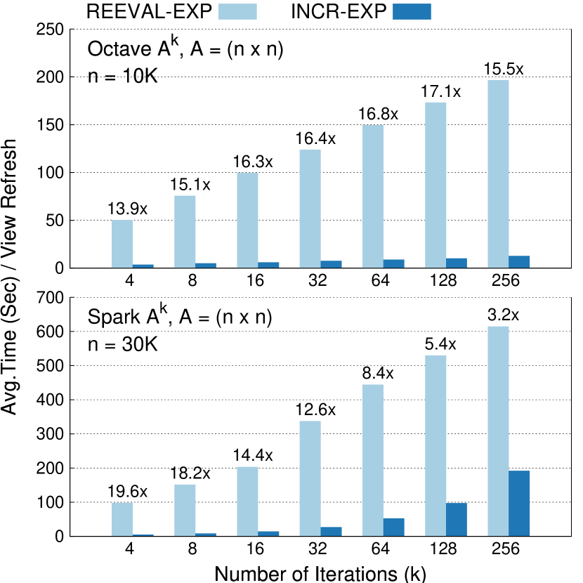
(c) Scalability of Powers $(k)$

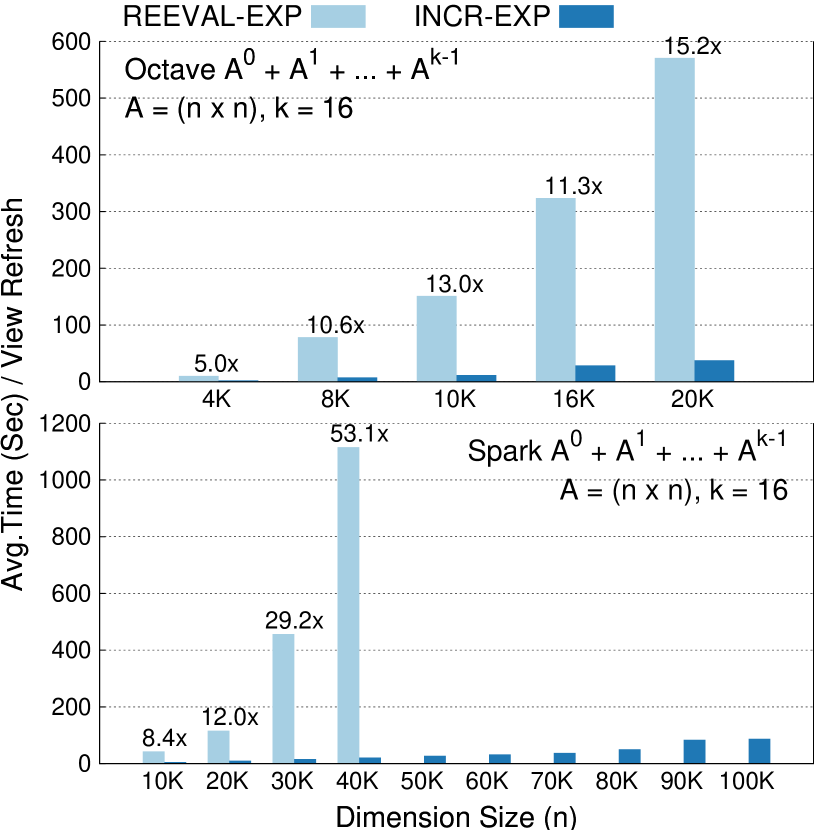
(d) Sums of Powers

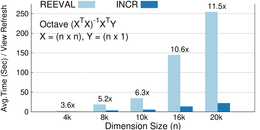
(e) Ordinary Least Squares

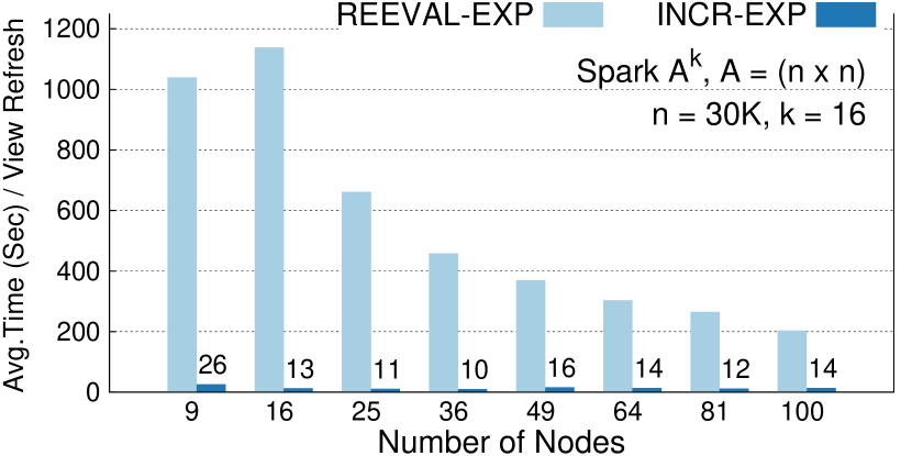
(f) Scalability of Powers (nodes)

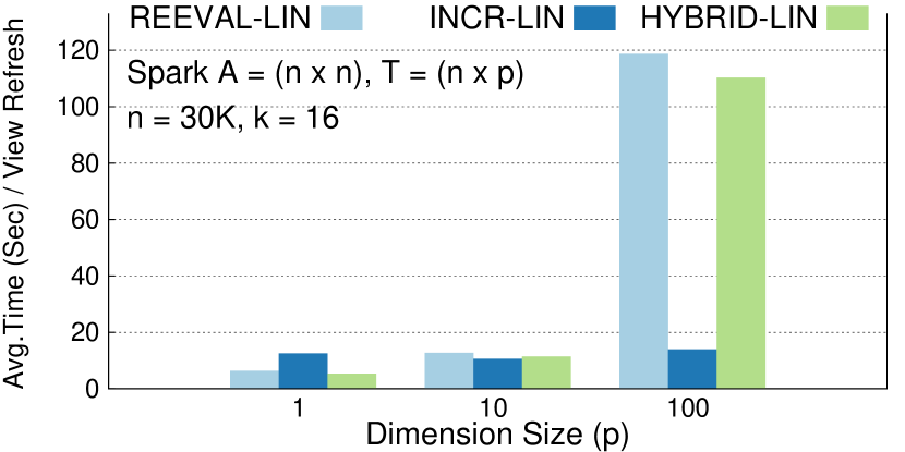
(g) $T_{i+1}=AT_{i}$

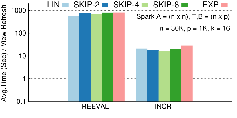
(h) LR: $T_{i+1}=AT_{i}+B$

Figure 3: Performance Evaluation of Incremental Maintenance using Octave and Spark

We have built the Linview system that implements incremental maintenance of analytical queries written as (iterative) linear algebra programs. It is a compilation framework that transforms a given program, based on the techniques discussed above, into efficient update triggers optimized for the execution on different runtime engines. Fig. 2 gives an overview of the system.

Workflow. The Linview framework consists of several compilation stages: the system transforms the code written in APL-style languages (e.g., R, MATLAB, Octave) into an abstract syntax tree (AST), performs incremental compilation, optimizes produced update triggers, and generates efficient code for execution on single-node (e.g., MATLAB) or parallel processing platforms (e.g., Spark, Mahout, Hadoop). The generated code consists of trigger functions for changes in each input matrix used in the original program.

The optimizer analyzes intra- and inter-statement dependencies in the input program and performs transformations, like common subexpression elimination and copy propagation [28], to reduce the overall maintenance cost. In this process, the optimizer might define a number of auxiliary materialized views that are maintained during runtime to support efficient processing of the trigger functions.

Extensibility. The Linview framework is also extensible: one may add new frontends to transform different input languages into AST or new backends that generate code for various execution environments. At the moment, Linview supports generation of Octave programs that are optimized for execution in multiprocessor environments, as well as Spark code for execution on large-scale cluster platforms. The experimental section presents results for both backends.

Distributed Execution. The competitive advantage of incremental computation over re-evaluation – reduced computation time – is even more pronounced in distributed environments. Generated incremental programs are amenable to distributed execution as they are composed of the standard matrix operations, for which many specialized tools offer scalable implementations, like ScaLAPACK, Intel MKL, and Mahout. In addition, by transforming expensive matrix operations to work with smaller datasets and representing changes in factored form, our incremental techniques also minimize the communication cost as less data has to be shipped over the network.

Data Partitioning. Linview analyzes data flow dependencies and data access patterns in a generated incremental program to decide on a partitioning scheme that minimizes data movement. A frequently occurring expression in trigger programs is a multiplication of a large matrix and a small delta matrix, typically performed in both directions (e.g., $A\,\Delta{A}$ and $\Delta{A}\,A$ in Example 1.1). To keep such computations strictly local, Linview partitions large matrices both horizontally and vertically, that is, each node contains one block of rows and one block of columns of a given matrix. Although such a hybrid partitioning strategy doubles the memory consumption, it allows the system to avoid expensive reshuffling of large matrices, requiring only small delta vectors or low-rank matrices to be communicated.

7 Experiments

This section demonstrates the potential of Linview over traditional re-evaluation techniques by comparing the average view refresh time for common data mining programs under a continuous stream of updates. We have built an APL-style frontend where users can provide their programs and annotate dynamic matrices. The Linview backend consists of two code generators capable of producing Octave and Spark executable code, optimized for the execution in multiprocessor and distributed environments.

For both Spark and Octave backends, our results show that: a) Incremental view maintenance outperforms traditional re-evaluation in almost all cases, validating the complexity results of Section 5; b) The performance gap between re-evaluation and incremental computation increases with higher dimensions; c) The hybrid evaluation strategy from Section 5.3, which combines re-evaluation and incremental computation, exhibits best performance when the input matrices are not large enough to justify the factored delta representation.

Experimental setup. To evaluate Linview’s performance using Octave, we run experiments on a $2.66$GHz Intel Xeon with $2\times 6$ cores, each with $2$ hardware threads, $64$GB of DDR$3$ RAM, and Mac OS X Lion 10.7.5. We execute the generated code using GNU Octave v$3.6.4$, an APL-style numerical computation framework, which relies on the ATLAS library for performing multi-threaded BLAS operations.

For large-scale experiments, we use an Amazon EC2 cluster with $26$ compute-optimized instances (c3.8xlarge). Each instance has $32$ virtual CPUs, each of them is a hardware hyper-thread from a $2.8$GHz Intel Xeon E5-2680v2 processor, $60$GB of RAM, and $2\times 320$GB SSD. The instances are placed inside a non-blocking $10$ Gigabit Ethernet network.

We run our experiments on top of the Spark engine – an in-memory parallel processing framework for large-scale data analysis. We configure Spark to launch $4$ workers on one EC2 instance – $100$ workers in total, each with $8$ virtual CPUs and $13.6$GB of RAM – and one master node on a separate EC2 instance. The generated Spark code relies on Jblas for performing matrix operations in Java. The Jblas library is essentially a wrapper around the BLAS and LAPACK routines. For the purpose of our experiments, we compiled Jblas with AMD Core Math Library v5.3.1 (ACML) – AMD’s BLAS implementation optimized for high performance. Jblas uses the ACML native library only for $\mathcal{O}(n^{\gamma})$ operations, like matrix multiplication.

We implement matrix multiplication on top of Spark using the simple parallel algorithm [16], and we partition input matrices in a $10\times 10$ grid. For the scalability test we use square grids of smaller sizes. For incremental evaluation, which involves multiplication with low-rank matrices, we use the data partitioning scheme explained in Section 6; we split the data horizontally among all available nodes, then broadcast the smaller relation to perform local computations, and finally concatenate the result at the master node. The Spark framework carries out the data shuffling among nodes.

Workload. Our experiments consider dense random matrices up to $(100\mbox{K}\times 100\mbox{K})$ in size, containing up to $10$ billion entries. All matrices have double precision and are preconditioned appropriately for numerical stability. For incremental evaluation, we also precompute the initial values of all auxiliary views and preload these values before the actual computation. We generate a continuous random stream of rank-$1$ updates where each update affects one row of an input matrix. On every such change, we re-evaluate or incrementally maintain the final result. The reported values show the average view refresh time over $3$ runs; the standard deviation was less than $5$% in each experiment.

Notation. Throughout the evaluation discussion we use the following notation: a) The prefixes Reeval, Incr, and Hybrid denote traditional re-evaluation, incremental processing, and hybrid computation, respectively; b) The suffixes Lin, Exp, and Skip-s represent the linear, exponential, and skip-$s$ models, respectively. These evaluation models are described in detail in Section 5 and Table 2.

Ordinary Least Squares. We conduct a set of experiments to evaluate the statistical estimator $\beta^{*}$ using OLS as defined in Section 5.1. Exceptionally in this example, we present only the Octave results as the current Spark backend lacks the support for re-evaluation of matrix inversion. The predictors matrix $X$ has dimension $(n\times n)$ and the responses matrix $Y$ is of dimension $(n\times p)$. Given a continuous stream of updates on $X$, Fig. 3(e) compares the average execution time of re-evaluation Reeval and incremental maintenance Incr of $\beta^{*}$ with different sizes of $n$. We set $p=1$ because this setting represents the lowest cost for Reeval, as the cost is dominated by the matrix inversion re-evaluation $\mathcal{O}(n^{\gamma})$. The graph illustrates the superiority of Incr over Reeval in computing the OLS estimates. Notice the asymptotically different behavior of these two graphs – the performance gap between Reeval and Incr increases with matrix size, from $3.56$x for $n=4,000$ to $11.45$x for $n=20,000$. This is consistent with the complexity results from Section 5.1.

Matrix Powers. We analyze the performance of the matrix powers $A^{k}$ evaluation, where $A$ has dimension $(n\times n)$, by varying different parameters of the computational model. First, we evaluate the performance of the evaluation strategies presented in Section 5.2, for a fixed dimension size and number of iterations $k=16$. Fig. 3(a) illustrates the average view refresh time of Octave generated programs for $n=10,000$ and Spark generated programs for $n=30,000$. In both implementations, the results demonstrate the virtue of Incr over Reeval and the efficiency of IncrExp over IncrLin and IncrSkip-s.

Next, we explore various scalability aspects of the matrix powers computation. Fig. 3(b) reports on the Octave performance over larger dimension sizes $n$, given a fixed number of iteration steps $k=16$; Fig. 3(b) also illustrates the Spark performance for even larger matrices. In both cases, IncrExp outperforms ReevalExp with similar asymptotic behavior. As in the OLS example, the performance gap increases with higher dimensionality.

Fig. 3(b) shows the Spark re-evaluation results for matrices up to size $n=50,000$. Beyond this limit, the running time of re-evaluation exceeds one hour due to an increased communication cost and garbage collection time. The re-evaluation strategy has a more dynamic model of memory usage due to frequent allocation and deallocation of large memory chunks as the data gets shuffled among nodes. In contrast, incremental evaluation avoids expensive communication by sending over the network only relatively small matrices. Up until $n=90,000$, we see a linear increase in the IncrExp running time. However, as discussed in Section 5, we expect the $\mathcal{O}{(n^{2})}$ complexity for incremental evaluation. The explanation lies in that the generated Spark code distributes the matrix-vector computation among many nodes and, inside each node, over multiple available cores, effectively achieving linear scalability. For $n=100,000$, incremental evaluation hits the resource limit in this cluster configuration, causing garbage collection to increase the average view refresh time.

Matrix Size		$20$K	$30$K	$40$K	$50$K
Memory	ReevalExp	$8.9$	$20.1$	$35.8$	$55.9$
(GB)	IncrExp	$29.8$	$67.1$	$119.2$	$186.3$
Time	ReevalExp	$95.0$	$203.4$	$667.3$	$1328.7$
(sec)	IncrExp	$9.6$	$14.1$	$21.0$	$24.9$
Speedup vs. Memory Cost		$2.99$	$4.31$	$9.55$	$16.00$

Table 3: The memory requirements and Spark view refresh times of ReevalExp and IncrExp for $A^{16}$ and different matrix sizes. The last row is the ratio between the speedup and memory overhead incurred by maintaining auxiliary views.

Memory Requirements. Table 3 presents the memory requirements and Spark single-update execution times of ReevalExp and IncrExp for the $A^{16}$ computation and various matrix dimensions. The last row represents the ratio between the speedup achieved using incremental evaluation and the memory overhead imposed by maintaining the results of intermediate iterations. We conclude that the benefit of investing more memory resources increases with higher dimensionality of the computation.

Next, we evaluate the scalability of the matrix powers computation for different numbers of Spark nodes. We evaluate various square grid configurations for re-evaluation of $A^{16}$, where $n=30,000$. Fig. 3(f) shows that our Spark implementation of matrix multiplication scales with more nodes. Also note that incremental evaluation is less susceptible to the number of nodes than re-evaluation; the average time per view refresh varies from 10 to 26 seconds.

Finally, in Fig. 3(c), we vary the number of iteration steps $k$ given a fixed dimension, $n=10,000$ for Octave and $n=30,000$ for Spark. The Octave performance gap between IncrExp and ReevalExp increases with more iterations up to $k=256$ when the size of the delta vectors $(10,000\times 256)$ becomes comparable with the matrix size. The Spark implementation broadcasts these delta vectors to each worker, so the achieved speedups decrease with larger iteration numbers due to the increased communication costs. However, as argued in Section 5.2, many iterative algorithms in practice require only a few iterations to converge, and for those the communication costs stay low.

Sums of Powers. We analyze the computation of sums of matrix powers, as described in Section 5.2.3. Since it shares the same complexity as the matrix powers computation, we present only the performance of the exponential models. Fig. 3(d) compares IncrExp and ReevalExp on various dimension sizes $n$ using Octave and Spark, for a given fixed number of iterations $k=16$. Similarly to the matrix powers results from Fig. 3(b), IncrExp outperforms traditional ReevalExp, and the achieved speedup increases with $n$. Beyond $n=40,000$, the Spark re-evaluation exceeds the one-hour time limit.

General Form. We evaluate the general iterative model of computation $T_{i+1}=A\,T_{i}+B$, where $T_{n\times p}$, $A_{n\times n}$, and $B_{n\times p}$, using the following settings (due to space constraints we show only important Spark results):

$\bullet$ B=0. The iterative computation degenerates to $T_{i+1}=A\,T_{i}$, which represents matrix powers when $p=n$, and thus we explore an alternative setting of $1\leq p<n$. For small values of $p$, the Lin model has the lowest complexity as it avoids expensive $\mathcal{O}{(n^{\gamma})}$ matrix multiplications. Fig. 3(g) shows the results of different evaluation strategies, given a fixed dimension $n=30,000$ and iteration steps $k=16$. For $p=1$, HybridLin outperforms ReevalLin by $16\%$ and IncrLin by $53\%$. However, the evaluation cost of both HybridLin and ReevalLin increases linearly with $p$. IncrLin exhibits the best performance among them when $p$ is large enough to justify the factored delta representation.

$\bullet$ B$\neq$0. We study an analytical query evaluating linear regression using the gradient descent algorithm of the form $\Theta_{i+1}=\Theta_{i}-X^{T}(X\Theta_{i}-Y)$. We adapt this form to the general iterative model by substituting $A=I-X^{T}X$ and $B=X^{T}Y$, where $I$ represents the identity matrix. Fig. 3(h) shows the performance of different iterative models for both re-evaluation and incremental computation, given fixed sizes $n=30,000$ and $p=1,000$ and a fixed number of iterations $k=16$. Note the logarithmic scale on the $y$ axis. The Lin model exhibits the best re-evaluation performance; the Skip-4 model has the lowest view refresh time for incremental evaluation. Overall, incremental computation outperforms traditional re-evaluation by a factor of 36.7x.

Zipf factor	$5.0$	$4.0$	$3.0$	$2.0$	$1.0$	$0.0$
Octave (10K)	$6.3$	$6.8$	$7.5$	$10.9$	$68.4$	$236.5$
Spark (30K)	$28.1$	$41.5$	$67.3$	$186.1$	$508.9$	$1678.8$

Table 4: The average Octave and Spark view refresh times in seconds for IncrExp of $A^{16}$ and a batch of $1,000$ updates. The row update frequency is drawn from a Zipf distribution.

Batch updates. We analyze the performance of incremental matrix powers computation for batch updates. We simulate a use case in which certain regions of the input matrix are changed more frequently than the others, and the frequency of row updates is described using a Zipf distribution. Table 4 shows the performance of incremental evaluation for a batch of $1,000$ updates and different Zipf factors. As the row update frequency becomes more uniform, that is, more rows are affected by a given batch, IncrExp loses its advantage over ReevalExp because the delta matrices become larger and more expensive to compute and distribute. To put these results in the context, a single update of a $n=10,000$ matrix in Octave takes $99.1$ and $6.3$ seconds on average for ReevalExp and IncrExp; For one update of a $n=30,000$ matrix using Spark, ReevalExp and IncrExp take $203.4$ and $14.1$ seconds on average. We observe that the Spark implementation exhibits huge communication overhead, which significantly prolongs the running time. We plan to investigate this issue in our future work.

Appendix A Matrix Powers

We analyze the time complexity of incremental view maintenance and hybrid evaluation for the computation of matrix powers discussed in Section 5 for rank-$1$ updates to $A$, denoted by $\Delta{A}=u\,v^{\text{T}}$. The analysis considers the three iterative models of computation from Section 3.

$\bullet$  In the linear model, $\Delta{P_{1}}=u\,v^{\text{T}}$, thus $U_{1}=u$ and $V_{1}=v$. For $i>1$,

$$\Delta{P_{i}}=\begin{bmatrix}U_{1}&(A\,U_{i-1}+U_{1}\,(V_{1}^{\text{T}}\,U_{i-1}))\end{bmatrix}\,\begin{bmatrix}V_{1}^{\text{T}}\,P_{i-1}\\ V_{i-1}^{\text{T}}\end{bmatrix}$$

where $U_{i}$ and $V_{i}$ are $(n\times i)$ block matrices (provable by induction), and $A$ and $P_{i}$ are $(n\times n)$ matrices. The evaluation cost of $P_{i}$, when $i>1$, is:

$$cost_{\textsc{Lin}}(P_{i}) =cost(U_{i})+cost(V_{i})+cost(U_{i}\,V_{i}^{\text{T}})$$

$$=2n^{2}i+3n(i-1).$$

The evaluation cost of all iterations in program $\mathcal{P}$ is

$$cost_{\textsc{Lin}}(\mathcal{P}) =n^{2}+\sum_{i=2}^{k}(2n^{2}i+3n(i-1))$$

$$=n^{2}(k^{2}+k-1)+\frac{3}{2}nk(k-1)=\mathcal{O}(n^{2}k^{2}).$$

$\bullet$  In the exponential model, $\Delta{P_{1}}=u\,v^{\text{T}}$, thus $U_{1}=u$ and $V_{1}=v$. For $i>1$,

$$\Delta{P_{i}}=\begin{bmatrix}U_{i/2}&(P_{i/2}\,U_{i/2}+U_{i/2}\,(V_{i/2}^{\text{T}}\,U_{i/2}))\end{bmatrix}\,\begin{bmatrix}V_{i/2}^{\text{T}}\,P_{i/2}\\ V_{i/2}^{\text{T}}\end{bmatrix}$$

where $U_{i}$ and $V_{i}$ are $(n\times i)$ block matrices, and $P_{i}$ is an $(n\times n)$ matrix. The evaluation cost of $P_{i}$, when $i>1$, is

$$cost_{\textsc{Exp}}(P_{i}) =cost(U_{i})+cost(V_{i})+cost(U_{i}\,V_{i}^{\text{T}})$$

$$=2n^{2}i+n\left(\frac{i^{2}}{2}+\frac{i}{2}\right).$$

The evaluation cost of all iterations in program $\mathcal{P}$ is:

$$cost_{\textsc{Exp}}(\mathcal{P}) =n^{2}+\sum_{i=2,4,8,\ldots k}(2n^{2}i+n\frac{i^{2}}{2}+n\frac{i}{2})$$

$$=n^{2}(4k-3)+n\frac{(k-1)(2k+5)}{3}=\mathcal{O}(n^{2}k).$$

$\bullet$  In the skip model, we first evaluate $T_{s}$ using the exponential model in $\mathcal{O}(n^{2}s)$ time as discussed above. Then $\Delta{P_{s}}=U_{s}\,V_{s}^{\text{T}}$, where $U_{s}$ and $V_{s}$ are $(n\times s)$ block matrices. For $i>s$,

$$\Delta{P_{i}}=\begin{bmatrix}U_{s}&(P_{s}\,U_{i-s}+U_{s}\,(V_{s}^{\text{T}}\,U_{i-s}))\end{bmatrix}\,\begin{bmatrix}V_{s}^{\text{T}}\,P_{i-s}\\ V_{i-s}^{\text{T}}\end{bmatrix}$$

where $U_{i}$ and $V_{i}$ are $(n\times i)$ block matrices, and $P_{i}$ is an $(n\times n)$ matrix. The evaluation cost of $P_{i}$, when $i>s$, is

$$cost_{\textsc{Skip}}(P_{i}) =cost(U_{i})+cost(V_{i})+cost(U_{i}\,V_{i}^{\text{T}})$$

$$=2n^{2}i+n(2s+1)(i-s).$$

The evaluation cost of all iterations in program $\mathcal{P}$ is

$$cost_{\textsc{Skip}}(\mathcal{P}) =\mathcal{O}(n^{2}s)+\sum_{i=2s,3s,\ldots k}(2n^{2}i+n(2s+1)(i-s))$$

$$=\mathcal{O}(n^{2}s)+\mathcal{O}\left(n^{2}\frac{k^{2}}{s}\right)=\mathcal{O}\left(n^{2}\frac{k^{2}}{s}\right).$$

Appendix B General Form: T_i+1 = AT_i + B

We analyze the time complexity of incremental view maintenance for the computation of matrix powers discussed in Section 5 for rank-$1$ updates to $A$, denoted by $\Delta{A}=u\,v^{\text{T}}$. The analysis considers the three iterative models of computation from Section 3.

The incremental strategy maintains the result of $T_{i}$, and if needed $P_{i}$ and $S_{i}$, for updates to $A$, denoted by $\Delta{A}=u\,v^{\text{T}}$. The delta expressions are in the factored form as $\Delta{T_{i}}=U_{i}\,V_{i}$, $\Delta{P_{i}}=Q_{i}\,R_{i}^{\text{T}}$, and $\Delta{S_{i}}=Z_{i}\,W_{i}^{\text{T}}$.

$\bullet$  In the linear model, $\Delta{A}=u\,v^{\text{T}}$, thus $U_{1}=u$ and $V_{1}=T_{0}^{\text{T}}\,v$. For $i>1$,

$$\Delta{T_{i}}=\begin{bmatrix}u&(A\,U_{i-1}+u\,(v^{\text{T}}\,U_{i-1}))\end{bmatrix}\,\begin{bmatrix}v^{\text{T}}\,T_{i-1}\\ V_{i-1}^{\text{T}}\end{bmatrix}$$

where $U_{i}=(n\times i)$ and $V_{i}=(p\times i)$ (provable by induction). The evaluation cost of $T_{i}$, when $i>1$, is

$$cost_{\textsc{Lin}}(T_{i}) =cost(U_{i})+cost(V_{i})+cost(U_{i}\,V_{i}^{\text{T}})$$

$$=n^{2}(i-1)+3n(i-1)+np(i+1).$$

The evaluation cost of all iterations in program $\mathcal{P}$ is

$$cost_{\textsc{Lin}}(\mathcal{P}) =2np+\sum_{i=2}^{k}(n^{2}(i-1)+np(i+1)+\mathcal{O}(ni))$$

$$=\mathcal{O}((n^{2}+np)k^{2}).$$

$\bullet$  In the exponential model, $\Delta{A}=u\,v^{\text{T}}$, thus $U_{1}=u$ and $V_{1}=T_{0}^{\text{T}}\,v$. Let $\Delta{P_{i}}=Q_{i}\,R_{i}^{\text{T}}$ and $\Delta{S_{i}}=Z_{i}\,W_{i}^{\text{T}}$. For $i>1$,

$$U_{i}=\begin{bmatrix}Q_{i/2}&(P_{i/2}\,U_{i/2}+Q_{i/2}\,(R_{i/2}^{\text{T}}\,U_{i/2}))&Z_{i/2}\end{bmatrix}$$

$$V_{i}=\begin{bmatrix}T_{i/2}^{\text{T}}\,R_{i/2}&V_{i/2}&B^{\text{T}}\,dW_{i/2}\end{bmatrix}$$

where $U_{i}=(n\times(2i-1))$ and $V_{i}=(p\times(2i-1))$. The evaluation cost of $T_{i}$, when $i>1$, disregarding the computation of $P_{i}$ and $S_{i}$, is

$$cost_{\textsc{Exp}}(T_{i}) =cost(U_{i})+cost(V_{i})+cost(U_{i}\,V_{i}^{\text{T}})$$

$$=n^{2}(i-1)+np(3i-1)+n(i+1)(i-1).$$

The evaluation cost of all iterations in program $\mathcal{P}$ is

$$cost_{\textsc{Exp}}(\mathcal{P})= \mathcal{O}(kn^{2})+$$

$$\sum_{i=2,4,\ldots k}\!\!\!\!\!(n^{2}(i-1)+np(3i-1)+\mathcal{O}(ni^{2}))$$

$$= \mathcal{O}((n^{2}+np)k).$$

$\bullet$  In the skip model, we first evaluate $T_{s}$ using the exponential model in $\mathcal{O}(s(n^{2}+np))$ time as discussed above. Then $\Delta{T_{s}}=U_{s}\,V_{s}^{\text{T}}$, where $U_{s}$ and $V_{s}$ are $(n\times(2s-1))$ block matrices. For $i>s$,

$$\Delta{T_{i}}=\begin{bmatrix}Q_{s}&(P_{s}\,U_{i-s}+Q_{s}\,(R_{s}^{\text{T}}\,U_{i-s}))&Z_{s}\end{bmatrix}\,\begin{bmatrix}R_{s}^{\text{T}}\,T_{i-s}\\ V_{i-s}^{\text{T}}\\ W_{s}^{\text{T}}\,B\end{bmatrix}$$

where $U_{i}$ and $V_{i}$ are $(n\times(2i-1))$ block matrices. The evaluation cost of $T_{i}$, when $i>s$, disregarding the computation of $P_{i}$ and $S_{i}$, is

$$cost_{\textsc{Skip}}(T_{i}) =cost(U_{i})+cost(V_{i})+cost(U_{i}\,V_{i}^{\text{T}})$$

$$=(2n^{2}(i-s)-1)+np(2i-1)+\mathcal{O}(n).$$

The evaluation cost of all iterations in program $\mathcal{P}$ is

$$cost_{\textsc{Skip}}(\mathcal{P})= \mathcal{O}((n^{2}+np)\log{s})+$$

$$\sum_{i=2s,3s,\ldots k}\!\!\!\!\!(n^{2}(2(i-s)-1)+np(2i-1)+\mathcal{O}(n))$$

$$= \mathcal{O}((n^{2}+np)\log{s})+\mathcal{O}\left((n^{2}+np)\frac{k^{2}}{s}\right)$$

$$= \mathcal{O}\left((n^{2}+np)\frac{k^{2}}{s}\right).$$

We analyze the cost of the hybrid evaluation strategy.

$\bullet$  In the linear model, $\Delta{A}=u\,v^{\text{T}}$ and $\Delta{T_{1}}=\Delta{A}\,T_{0}$. For $i>1$,

$$\Delta{T_{i}}=u\,v^{\text{T}}\,T_{i-1}+A\,\Delta{T_{i-1}}+u\,v^{\text{T}}\,\Delta{T_{i-1}}.$$

The evaluation cost of $T_{i}$, when $i>s$, is

$$cost_{\textsc{Lin}}(T_{i}) =cost(\Delta{T_{i}})=pn^{2}+6np.$$

The evaluation cost of all iterations in program $\mathcal{P}$ is

$$cost_{\textsc{Lin}}(\mathcal{P})=n^{2}+\sum_{i=2}^{k}(pn^{2}+6np)=\mathcal{O}(pn^{2}k).$$

$\bullet$  In the exponential model, $\Delta{A}=u\,v^{\text{T}}$ and $\Delta{T_{1}}=\Delta{A}\,T_{0}$. Let $\Delta{P_{i}}=Q_{i}\,R_{i}^{\text{T}}$ and $\Delta{S_{i}}=Z_{i}\,W_{i}^{\text{T}}$. For $i>1$,

$$\Delta{T_{i}}= Q_{i/2}\,R_{i/2}^{\text{T}}\,T_{i/2}+P_{i/2}\,\Delta{T_{i/2}}+$$

$$Q_{i/2}\,R_{i/2}^{\text{T}}\,\Delta{T_{i/2}}+Z_{i/2}\,W_{i/2}^{\text{T}}\,B.$$

The evaluation cost of $T_{i}$, when $i>1$, disregarding the computation of $P_{i}$ and $S_{i}$, is

$$cost_{\textsc{Exp}}(T_{i})=cost(\Delta{T_{i}})=pn^{2}+3np(i+1).$$

The evaluation cost of all iterations in program $\mathcal{P}$ is

$$cost_{\textsc{Exp}}(\mathcal{P}) =\mathcal{O}(n^{2}k)+\sum_{i=2,4,8,\ldots k}(pn^{2}+3np(i+1))$$

$$=\mathcal{O}(pn^{2}\log{k}+n^{2}k).$$

$\bullet$  In the skip model, we first evaluate $T_{s}$ using the exponential model in $\mathcal{O}(pn^{2}\log{s}+sn^{2})$ time as discussed above. For $i>s$,

$$\Delta{T_{i}}=Q_{s}\,R_{s}^{\text{T}}\,T_{i-s}+P_{s}\,\Delta{T_{i-s}}+Q_{s}\,R_{s}^{\text{T}}\,\Delta{T_{i-s}}+Z_{s}\,W_{s}^{\text{T}}\,B.$$

The evaluation cost of $T_{i}$, when $i>s$, disregarding the computation of $P_{i}$ and $S_{i}$, is

$$cost_{\textsc{Skip}}(T_{i})=cost(\Delta{T_{i}})=pn^{2}+6nps+3np.$$

The evaluation cost of all iterations in program $\mathcal{P}$ is

$$cost_{\textsc{Skip}}(\mathcal{P})= \mathcal{O}(pn^{2}\log{s}+n^{2}s)+$$

$$\sum_{i=2s,3s,\ldots k}(pn^{2}+6nps+3np)$$

$$= \mathcal{O}(pn^{2}\log{s}+n^{2}s)+\mathcal{O}\left(pn^{2}\frac{k}{s}\right)$$

$$= \mathcal{O}\left(pn^{2}\left(\log{s}+\frac{k}{s}\right)+n^{2}s\right).$$

References

- [1] D. Abadi, Y. Ahmad, M. Balazinska, M. Cherniack, J. Hwang, W. Lindner, A. Maskey, E. Rasin, E. Ryvkina, N. Tatbul, Y. Xing, and S. Zdonik. The design of the Borealis stream processing engine. In CIDR, 2005.
- [2] U. Acar, G. Blelloch, M. Blume, R. Harper, and K. Tangwongsan. An experimental analysis of self-adjusting computation. TOPLAS, 32(1), 2009.
- [3] A. Arasu, B. Babcock, S. Babu, J. Cieslewicz, K. Ito, R. Motwani, U. Srivastava, and J. Widom. Stream: the Stanford data stream management system. Technical report, Stanford InfoLab, 2004.
- [4] P. Baumann, A. Dehmel, P. Furtado, R. Ritsch, and N. Widmann. The multidimensional database system RasDaMan. In SIGMOD, 1998.
- [5] J. Berger. Statistical decision theory and Bayesian analysis. Springer, 1985.
- [6] P. Berkhin. A survey on PageRank computing. Internet Mathematics, 2(1), 2005.
- [7] J. Blakeley, P. Larson, and F. Tompa. Efficiently updating materialized views. In SIGMOD, 1986.
- [8] Y. Bu, B. Howe, M. Balazinska, and M. Ernst. HaLoop: Efficient iterative data processing on large clusters. PVLDB, 3(1), 2010.
- [9] Y. Chen, J. Dunfield, and U. Acar. Type-directed automatic incrementalization. In PLDI, 2012.
- [10] R. Chirkova and J. Yang. Materialized views. Foundations and Trends in Databases, 4(4), 2012.
- [11] H. Cohn, R. Kleinberg, B. Szegedy, and C. Umans. Group theoretic algorithms for matrix multiplication. In FOCS, 2005.
- [12] S. Das, Y. Sismanis, K. Beyer, R. Gemulla, P. Haas, and J. McPherson. Ricardo: Integrating R and Hadoop. In SIGMOD, 2010.
- [13] L. Deng. Multiple-rank updates to matrix factorizations for nonlinear analysis and circuit design. PhD thesis, Stanford University, 2010.
- [14] J. Dongarra, J. Du Croz, S. Hammarling, and I. Duff. A set of level 3 basic linear algebra subprograms. TOMS, 16(1), 1990.
- [15] J. Ekanayake, H. Li, B. Zhang, T. Gunarathne, S.-H. Bae, J. Qiu, and G. Fox. Twister: A runtime for iterative MapReduce. In HPDC, 2010.
- [16] A. Grama, G. Karypis, V. Kumar, and A. Gupta. Introduction to Parallel Computing (2nd Edition). Addison Wesley, 2003.
- [17] A. Gupta and I. Mumick. Materialized Views. MIT Press, 1999.
- [18] J. Hellerstein, C. Ré, F. Schoppmann, D. Z. Wang, E. Fratkin, A. Gorajek, K. Ng, C. Welton, X. Feng, K. Li, and A. Kumar. The MADlib analytics library or MAD skills, the SQL. PVLDB, 5(12), 2012.
- [19] M. Isard, M. Budiu, Y. Yu, A. Birrell, and D. Fetterly. Dryad: Distributed data-parallel programs from sequential building blocks. In EuroSys, 2007.
- [20] S. Kamvar, T. Haveliwala, and G. Golub. Adaptive methods for the computation of PageRank. Technical report, Stanford University, 2003.
- [21] C. Koch, Y. Ahmad, O. Kennedy, M. Nikolic, A. Nötzli, D. Lupei, and A. Shaikhha. DBToaster: Higher-order delta processing for dynamic, frequently fresh views. VLDBJ, 23(2), 2014.
- [22] T. Kraska, A. Talwalkar, J. Duchi, R. Griffith, M. Franklin, and M. Jordan. MLbase: A distributed machine-learning system. In CIDR, 2013.
- [23] A. Langville and C. Meyer. Deeper inside PageRank. Internet Mathematics, 1(3), 2004.
- [24] A. Marathe and K. Salem. Query processing techniques for arrays. VLDBJ, 11(1), 2002.
- [25] F. McSherry, D. Murray, R. Isaacs, and M. Isard. Differential dataflow. In CIDR, 2013.
- [26] S. Mihaylov, Z. Ives, and S. Guha. REX: Recursive, delta-based data-centric computation. PVLDB, 5(11), 2012.
- [27] R. Motwani, J. Widom, A. Arasu, B. Babcock, S. Babu, M. Datar, G. Manku, C. Olston, J. Rosenstein, and R. Varma. Query processing, approximation, and resource management in a data stream management system. In CIDR, 2003.
- [28] S. Muchnick. Advanced Compiler Design and Implementation. Morgan Kaufmann, 1997.
- [29] W. Press, S. Teukolsky, W. Vetterling, and B. Flannery. Numerical Recipes 3rd Edition: The Art of Scientific Computing. Cambridge University Press, 2007.
- [30] M. Seeger. Low rank updates for the Cholesky decomposition. Technical report, EPFL, 2004.
- [31] M. Stonebraker, C. Bear, U. Cetintemel, M. Cherniack, T. Ge, N. Hachem, S. Harizopoulos, J. Lifter, J. Rogers, and S. Zdonik. One size fits all? Part 2: Benchmarking results. In CIDR, 2007.
- [32] M. Stonebraker, J. Becla, D. DeWitt, K. Lim, D. Maier, O. Ratzesberger, and S. Zdonik. Requirements for science data bases and SciDB. In CIDR, 2009.
- [33] S. Venkataraman, I. Roy, A. AuYoung, and R. Schreiber. Using R for iterative and incremental processing. In HotCloud, 2012.
- [34] C. Whaley and J. Dongarra. Automatically tuned linear algebra software. In PPSC, 1999.
- [35] M. Zaharia, M. Chowdhury, M. Franklin, S. Shenker, and I. Stoica. Spark: Cluster computing with working sets. In HotCloud, 2010.
- [36] C. Zhang, A. Kumar, and C. Ré. Materialization optimizations for feature selection workloads. In SIGMOD, 2014.
- [37] Y. Zhang, Q. Gao, L. Gao, and C. Wang. iMapReduce: A distributed computing framework for iterative computation. Journal of Grid Computing, 10(1), 2012.
- [38] Y. Zhang, H. Herodotou, and J. Yang. RIOT: I/O-efficient numerical computing without SQL. In CIDR, 2009.
- [39] Y. Zhang, M. Kersten, and S. Manegold. SciQL: Array data processing inside an RDBMS. In SIGMOD, 2013.