The shear modulus of glasses:
results from the full replica symmetry breaking solution

Abstract

We compute the shear modulus of amorphous hard and soft spheres, using the exact solution in infinite spatial dimensions that has been developed recently. We characterize the behavior of this observable in the whole phase diagram, and in particular around the glass and jamming transitions. Our results are consistent with other theoretical approaches, that are unified within this general picture, and they are also consistent with numerical and experimental results. Furthermore, we discuss some properties of the out-of-equilibrium dynamics after a deep quench close to the jamming transition, and we show that a combined measure of the shear modulus and of the mean square displacement allows one to probe experimentally the complex structure of phase space predicted by the full replica symmetry breaking solution.

I Introduction

Amorphous soft spheres with repulsive interaction, that are a good model for colloidal glasses, molecular glasses, and granular media Torquato and Stillinger (2010); Parisi and Zamponi (2010); Berthier and Biroli (2011), display a very complex rheological behavior, controlled by two distinct “critical” points: the glass transition and the jamming transition Ikeda et al. (2012); Parisi and Zamponi (2010). The control parameters for these systems are density (or better packing fraction $\varphi$) and temperature $T$ (or better the ratio $T/\epsilon$ between temperature $T$ and the typical interaction energy $\epsilon$). At densities below the glass transition, the system is liquid, hence it can flow and its shear modulus vanishes. At the glass transition, the system acquires a finite rigidity through a discontinuous transition at which the shear modulus jumps to a finite value Szamel and Flenner (2011); Yoshino (2012). Simultaneously the yield stress may also exhibit a similar discontinuous transition Ikeda et al. (2012); Fuchs and Cates (2002). It is important to stress that, at densities slightly above the glass transition and at low enough temperatures, rigidity has an entropic origin, as in a hard sphere crystal Mason and Weitz (1995); Ikeda et al. (2012). In fact, at zero temperatures, the spheres have enough room to fit in space without touching, hence they do not interact and the system is loose. At small finite temperature, however, the spheres vibrate and collide, giving rise to an effective interaction that makes the system rigid Brito and Wyart (2006). In this region of density, and in the limit of vanishing temperature, both the pressure and the shear modulus are therefore proportional to temperature. Upon further compression, the system reaches a “random close packing” or “jamming” density Pusey and Van Megen (1986); Bernal and Mason (1960); Liu et al. (2011); O’Hern et al. (2002). We denote $\varphi_{j}$ the packing fraction at the jamming point. Above this density, the spheres cannot fit in space without being “squeezed” by their neighbors, and rigidity and pressure acquire a mechanical origin, being due to a direct interaction between the particles Mason et al. (1997); Ikeda et al. (2012). Both pressure and the shear modulus, therefore, have a finite zero-temperature limit in the region $\varphi>\varphi_{j}$. Note that, as a consequence, infinitely hard particles cannot be compressed beyond the jamming point, because the mechanical repulsion becomes infinite and cannot be overcome by any finite pressure. Hard spheres can therefore be thought as a particular case of soft spheres with repulsive strength $\epsilon$, that is obtained by taking the limit $T/\epsilon\rightarrow 0$ for $\varphi<\varphi_{j}$. Obviously the limit $T/\epsilon\rightarrow 0$ can be taken equivalently by sending $T\rightarrow 0$ or $\epsilon\rightarrow\infty$ Ikeda et al. (2012, 2013); Berthier and Witten (2009); Berthier et al. (2011).

The interplay of the jamming and glass transitions gives rise to complex flow curves in the packing fraction-temperature ($\varphi$, $T$) plane, which have been the subject of many experimental, numerical and analytical investigations. A very complete characterization of the flow curves in the regime of interest for the present work has been reported in Ikeda et al. (2012). Concerning the behavior of the shear modulus $\mu$, most of the previous studies agree on two main qualitative observations. First, the shear modulus jumps discontinuously at the glass transition Ikeda et al. (2012); Yoshino (2012, 2013); Fuchs and Cates (2002); Szamel and Flenner (2011); secondly, it has a critical behavior around the jamming transition at $\varphi_{j}$ Brito and Wyart (2006); O’Hern et al. (2002); Zaccone and Scossa-Romano (2011); Wyart (2005); DeGiuli et al. (2014a). In fact, in the hard spheres regime when $T\rightarrow 0$ and $\varphi\rightarrow\varphi_{j}^{-}$, the shear modulus is proportional to $T$ and $\mu/T\sim(\varphi_{j}-\varphi)^{-\kappa}$, with $\kappa$ close to $3/2$ Brito and Wyart (2006). For soft harmonic spheres at $T=0$, when $\varphi\rightarrow\varphi_{j}^{+}$ the shear modulus vanishes as $\mu\sim(\varphi-\varphi_{j})^{\kappa^{\prime}}$ with $\kappa^{\prime}$ close to $1/2$ O’Hern et al. (2002); Wyart (2005). The exponent $\kappa$ has been related to other exponents that characterize criticality at the jamming transition DeGiuli et al. (2014a), whereas for soft spheres the prediction that $\kappa^{\prime}=1/2$ was made using different approximations Wyart (2005); DeGiuli et al. (2014b). Remarkably, despite the fact that both the glass and the jamming transition happen out-of-equilibrium, hence at protocol-dependent densities, the critical properties around these transitions are universal and independent of the protocol, for a wide range of reasonable preparation protocols Parisi and Zamponi (2010); Ikeda et al. (2012); Charbonneau et al. (2012); Lerner et al. (2013); DeGiuli et al. (2014a).

Constructing a first principle theory able to describe the complex rheological properties of these systems is a difficult task. One of the most successful theories is Mode-Coupling Theory (MCT) Götze (2009), that is based on an approximate set of dynamical equations. MCT predicts the existence of sharp dynamical glass transition on a line $T_{\rm d}(\varphi)$ that ends, for $T\rightarrow 0$, at density $\varphi_{\rm d}<\varphi_{j}$ Berthier and Witten (2009). For $T<T_{\rm d}(\varphi)$ (or $\varphi>\varphi_{\rm d}$ in the hard sphere limit $T/\epsilon\rightarrow 0$), diffusion is completely arrested and particles are completely caged by their neighbors. MCT can describe well the rheological properties around the glass transition Fuchs and Cates (2002); Szamel and Flenner (2011). However, MCT does not provide good results deep in the glass phase and in particular it fails to describe correctly the jamming transition Ikeda and Berthier (2013). Another first-principle approach to glass physics is based on the assumption that glasses are long-lived metastable states, and can be described by a restricted equilibrium thermodynamics. Concrete computations can then be done using replicas, and have been usually done within the so-called “1-step replica symmetry breaking” (1RSB) scheme Mezard and Parisi (2012); Parisi and Zamponi (2010). This method has been applied to describe the rigidity of structural glasses, including hard and soft sphere systems Yoshino and Mézard (2010); Yoshino (2012, 2013); Okamura and Yoshino (2013), and provides good qualitative and quantitative results for the shear modulus, but in the simplest 1RSB scheme it fails to predict the exponents $\kappa$ and $\kappa^{\prime}$ correctly Yoshino (2013); Okamura and Yoshino (2013). Both the MCT and the replica approach are thought to be part of the more general Random First Order Transition (RFOT) scenario for the glass transition Kirkpatrick and Wolynes (1987); Kirkpatrick and Thirumalai (1987); Kirkpatrick et al. (1989).

Following a well-established tradition in theoretical physics Witten (1980), in Kurchan et al. (2012, 2013); Charbonneau et al. (2013, 2014) a new approach was adopted by solving exactly the hard sphere model in the limit of $d\rightarrow\infty$, in which the RFOT scenario is exactly realized Kirkpatrick and Wolynes (1987). In particular, in Charbonneau et al. (2013, 2014) it was shown that in addition to the glass and jamming transitions, a new transition takes place deep in the glass phase and before jamming occurs. This so-called Gardner transition is a transition where the 1RSB structure changes into a full replica symmetry breaking (fullRSB) one Gardner (1985); Mézard et al. (1987). Physically, this corresponds to a splitting of glass basins into a complex hierarchy of subbasins, akin to the one of the Sherrington-Kirkpatrick model. This structure has been described in detail in the literature Mézard et al. (1987). In Charbonneau et al. (2013, 2014) it was shown that this exact solution predicts a phase diagram which is in very good qualitative agreement with the one observed in numerical simulations and experiments, and in particular it gives correct analytical predictions for the critical exponents that characterize the jamming transition. The solution, originally obtained for hard spheres, can be also extended to soft spheres at low enough temperatures in the vicinity of the jamming transition Berthier et al. (2011); Charbonneau et al. (2013).

The aim of this paper is to extend the analysis of Charbonneau et al. (2013) to describe the rheological properties of soft and hard spheres in the limit $d\rightarrow\infty$, and in particular to compute the shear modulus. Our main results are: (i) at the dynamic glass transition $\varphi_{\rm d}$, the shear modulus $\mu$ jumps discontinuously to a finite value, and at densities slightly above the transition it displays a square-root singularity $\mu\sim\mu_{\rm d}+C(\varphi-\varphi_{\rm d})^{1/2}$; (ii) the critical properties around the jamming transition $\varphi_{j}$ are the ones described above, with $\mu\sim T(\varphi_{j}-\varphi)^{-\kappa}$ for $\varphi\rightarrow\varphi_{j}^{-}$ with $\kappa=1.41575$, while the exponent $\kappa^{\prime}$ remains for the moment undetermined; (iii) we derive predictions for the out-of-equilibrium dynamics after a deep quench close to the jamming transition that are direct consequences of the fullRSB structure. Note that, as discussed in Charbonneau et al. (2013), non-trivial exponents emerge from the mean field computation due to the complex pattern of fullRSB. Our approach unifies, in a well controlled mean field setting, several theoretical approaches such as MCT Fuchs and Cates (2002); Szamel and Flenner (2011); Ikeda and Berthier (2013) and effective medium approaches Wyart (2005); Brito and Wyart (2006); DeGiuli et al. (2014a).

Whether these infinite-dimensional results can be immediately translated to experimental systems in $d=2,3$ is of course a crucial question that remains open from the purely theoretical point of view. However, the qualitative phase diagram is consistent with numerical results Ikeda et al. (2012), and the predicted critical exponents also agree well with numerical results O’Hern et al. (2002); Brito and Wyart (2006); Ikeda et al. (2012); Okamura and Yoshino (2013). Moreover, the method of solution that is exact in infinite dimensions can be used, in an approximate way, to provide quantitative predictions for non-universal quantities (such as the transition densities $\varphi_{\rm d}$ and $\varphi_{j}$, the equation of state of the glass, the correlation function, etc.) in finite dimensions Mezard and Parisi (2012); Parisi and Zamponi (2010); Berthier et al. (2011); Yoshino (2012), which agree well with numerical data. Despite all these positive results, several problems remain open and we discuss them in the conclusions.

II Shearing the molecular liquid

II.1 General formulation

In the following, we consider a system of $N$ identical particles in a cubic $d$ dimensional volume $V$, with density $\rho=N/V$. Particles interact through a two-body potential $v(r)$, which in most cases will be the hard sphere potential with diameter $D$. To keep the discussion more general, we consider also a generic soft potential with range $D$ and temperature $T=1/\beta$, defined as $v(r)=\epsilon(1-r/D)^{2}\theta(D-r)$, where $\theta(x)$ is the Heaviside step function. The hard sphere limit correspond to $\epsilon\rightarrow\infty$. We define the packing fraction $\varphi=\rho V_{d}(D/2)^{d}$, where $V_{d}$ is the volume of a $d$-dimensional sphere of unit radius Parisi and Zamponi (2010), and a scaled packing fraction $\widehat{\varphi}=\rho V_{d}D^{d}/d=2^{d}\varphi/d$. We consider first the thermodynamic limit $N\rightarrow\infty$, and then the limit $d\rightarrow\infty$, which is natural from the statistical mechanics point of view. Also, the inverse limit is ill-defined because a minimal number of particles $N\sim 2^{d}$ is needed to define properly the problem in dimension $d$ Charbonneau et al. (2011).

A general approach to compute properties of glasses through a “cloned liquid” replica method has been presented in Mezard and Parisi (2012), and applied to the computation of the shear modulus in Yoshino and Mézard (2010); Yoshino (2012). To keep this paper reasonably short, we cannot reproduce this construction here. We therefore assume that the reader is familiar with (i) the general formalism of the replica method of spin glasses, including the 1-step replica symmetry breaking (1RSB) and full replica symmetry breaking (fullRSB) schemes, reviewed e.g. in Castellani and Cavagna (2005); Mézard et al. (1987); (ii) the “cloned liquid” construction to compute properties of glasses, originally introduced in Monasson (1995); Mézard and Parisi (1996) and reviewed in Mezard and Parisi (2012), including its application to compute the shear modulus Yoshino (2012); (iii) its application to hard sphere systems, reviewed in Parisi and Zamponi (2010), and in particular the structure of the 1RSB solution in the limit $d\rightarrow\infty$ (Parisi and Zamponi, 2010, Sec.VI); (iv) the construction of a fullRSB solution for hard spheres in $d\rightarrow\infty$ and the associated phase diagram, obtained in Kurchan et al. (2012, 2013); Charbonneau et al. (2013).

To describe glassy states, we consider $m$ identical replicas of the original system Monasson (1995). To describe the fullRSB structure, we follow the results and the notations of Charbonneau et al. (2013), and we assume that the $m$ replicas all belong to one of the largest metabasins, in such a way that their mean square displacement is at most $\widehat{\Delta}_{1}$. As a consequence, the replicas form a molecular liquid in which each molecule contains one particle of each of the replicas.

Each molecule is described by a set of $m$ coordinates ${\overline{x}}=\{x_{1}\cdots x_{m}\}$, where $x_{a}$ are $d$-dimensional vectors. Following Yoshino and Mézard (2010); Yoshino (2012), we apply a shear-strain $\gamma_{a}$ to replica $a$, which is obtained by deforming linearly the volume in which the system is contained. We call $x^{\prime}_{\mu}$, with $\mu=1,\cdots,d$, the coordinates in the original reference frame, in which the shear-strain is applied. In this frame, the cubic volume is deformed because of shear-strain. To remove this undesirable feature, we introduce new coordinates $x_{\mu}$ of a “strained” frame in which the volume is brought back to a cubic shape. If the shear-strain is applied along direction $\mu=2$, then for replica $a$ all the coordinates are unchanged, $x_{a\mu}=x_{a\mu}^{\prime}$, except the first one which is changed according to

$$x_{a1}^{\prime}=x_{a1}+\gamma_{a}x_{a2}\ ,\hskip 30.0ptx_{a1}=x_{a1}^{\prime}-\gamma_{a}x_{a2}^{\prime}\ .$$ (1)

Let us call $S(\gamma_{a})$ the matrix such that $x_{a}^{\prime}=S(\gamma_{a})x_{a}$. In the original frame (where the volume is deformed by strain), two particles of replica $a$ interact with the potential $v(|x_{a}^{\prime}-y_{a}^{\prime}|)$. If we change variable to the strained frame (where the volume is not deformed), the interaction is

$$v_{\gamma_{a}}(x_{a}-y_{a})=v(|S(\gamma_{a})(x_{a}-y_{a})|)\ .$$ (2)

An important remark is that $\det S(\gamma)=1$ meaning that the simple shear-strain defined above does not change the volume and thus the average density $\rho=N/V$ of the system.

In $d\rightarrow\infty$, we keep only the first non-trivial term of the virial series Frisch and Percus (1999); Parisi and Zamponi (2010); Kurchan et al. (2012). Using the coordinates of the strained frame, the system is translationally invariant in the usual way and, following the same steps and notations of Kurchan et al. (2012), we can write the free energy of the replicated liquid as

$$\begin{split}-\beta NF(\{\gamma_{a}\})&=\int d\overline{x}\rho(\overline{x})[1-\log\rho(\overline{x})]+\frac{1}{2}\int d\overline{x}d\overline{y}\rho(\overline{x})\rho(\overline{y})f_{\{\gamma_{a}\}}(\overline{x}-\overline{y})\\ &=V\int{\cal D}\overline{u}\rho(\overline{u})[1-\log\rho(\overline{u})]+\frac{V}{2}\int{\cal D}\overline{u}{\cal D}\overline{v}\rho(\overline{u})\rho(\overline{v})\overline{f}_{\{\gamma_{a}\}}(\overline{u}-\overline{v})\ ,\end{split}$$ (3)

where $X=m^{-1}\sum_{a}x_{a}$ is the center of mass of a molecule, $u_{a}=x_{a}-X$ is the displacement of replica $a$ in the molecule, the Mayer function is

$$f_{\{\gamma_{a}\}}(\overline{x}-\overline{y})=-1+\prod_{a=1}^{m}e^{-\beta v(|S(\gamma_{a})(x_{a}-y_{a})|)}=f(\{S(\gamma_{a})(x_{a}-y_{a})\})\ ,$$ (4)

$f(\overline{x}-\overline{y})$ is the usual Mayer function that was considered in Kurchan et al. (2012), and $\overline{f}_{\{\gamma_{a}\}}(\overline{u}-\overline{v})=\int dXf_{\{\gamma_{a}\}}(X+\overline{u}-\overline{v})$ is the translationally averaged Mayer function as in Kurchan et al. (2012).

Following Yoshino and Mézard (2010); Yoshino (2012), we want to develop the free energy for small $\gamma_{a}$, and we define

$$F(\{\gamma_{a}\})=F(\{0\})+\sum_{a=1}^{m}\sigma_{a}\gamma_{a}+\frac{1}{2}\sum_{a,b}^{1,m}\mu_{ab}\gamma_{a}\gamma_{b}+\cdots$$ (5)

which defines the shear modulus matrix $\mu_{ab}$, whose physical interpretation will be discussed later.

II.2 Replicated Mayer function in presence of shear-strain

Clearly, the shear-strain $\gamma_{a}$ enters only in the second term of Eq. (3), that represents the mean field density-density interaction, and for this reason we call it the “interaction term” Kurchan et al. (2012). We shall therefore repeat the steps of (Kurchan et al., 2012, Sec. 5) in presence of the shear-strain.

We specialize here to hard spheres for simplicity, but the derivation can be easily extended to soft spheres following the analysis of Ref. Charbonneau et al. (2013). Taking into account translational invariance following the same steps as in Kurchan et al. (2012), we obtain a modified Mayer function that reads

$$\overline{f}_{\{\gamma_{a}\}}(\bar{u})=\int dX\left\{-1+\prod_{a=1}^{m}\theta(|S(\gamma_{a})(X+u_{a})|-D)\right\}=-\int dX\,\theta(D-\min_{a}|S(\gamma_{a})(X+u_{a})|)\ ,$$ (6)

where $\theta(x)$ is the Heaviside step function. This function is integrated over $\bar{u}-\bar{v}$ in Eq. (3), where $\bar{u}$ and $\bar{v}$ are extracted from the density distribution $\rho(\bar{u})$. Here we shift $u_{a}-v_{a}\rightarrow u_{a}$. The $m$ vectors $u_{a}$ define an $m$-dimensional plane in the $d$-dimensional space, and because the vectors $u_{a}$ are extracted at random, this plane is orthogonal to the shear-strain directions $\mu=1,2$ with probability going to 1 for $d\rightarrow\infty\gg m$. Hence, the vector $X$ can be decomposed in a two dimensional vector $\{X_{1},X_{2}\}$ parallel to the shear-strain plane, a $(d-m-2)$-component vector $X_{\perp}$, orthogonal to the plane $\mu=1,2$ and to the plane defined by $u_{a}$, and a $m$-component vector $X_{\parallel}$ parallel to that plane. Defining $\Omega_{d}$ as the $d$-dimensional solid angle and recalling that $V_{d}=\Omega_{d}/d$, and following the same steps as in (Kurchan et al., 2012, Sec. 5), we have

$$\begin{split}\overline{f}_{\{\gamma_{a}\}}(\bar{u})&=-\int dX\,\theta(D^{2}-\min_{a}|S(\gamma_{a})(X+u_{a})|^{2})\\ &=-\int dX_{1}dX_{2}\ d^{m}X_{\parallel}\ d^{d-m-2}X_{\perp}\ \theta(D^{2}-\min_{a}\{(X_{1}+\gamma_{a}X_{2})^{2}+X_{2}^{2}+|X_{\parallel}+u_{a}|^{2}+|X_{\perp}|^{2}\})\\ &=-\Omega_{d-m-2}\int dX_{1}dX_{2}\ d^{m}X_{\parallel}\int_{0}^{\infty}dx\,x^{d-m-3}\,\theta(D^{2}-x^{2}-\min_{a}\{(X_{1}+\gamma_{a}X_{2})^{2}+X_{2}^{2}+|X_{\parallel}+u_{a}|^{2}\})\\ &=-\Omega_{d-m-2}\int dX_{1}dX_{2}\ d^{m}X_{\parallel}\int_{0}^{\sqrt{D^{2}-\min_{a}\{(X_{1}+\gamma_{a}X_{2})^{2}+X_{2}^{2}+|X_{\parallel}+u_{a}|^{2}\}}}dx\,x^{d-m-3}\\ &=-V_{d-m-2}\int dX_{1}dX_{2}\ d^{m}X_{\parallel}\,\Theta_{d-m-2}(D^{2}-\min_{a}\{(X_{1}+\gamma_{a}X_{2})^{2}+X_{2}^{2}+|X_{\parallel}+u_{a}|^{2}\})\end{split}$$ (7)

where we defined the function Kurchan et al. (2012)

$$\Theta_{n}(x)=x^{n/2}\theta(x)\ .$$ (8)

It has been shown in Kurchan et al. (2012) that the region where $\overline{f}_{\{\gamma_{a}\}}(\bar{u})$ has a non-trivial dependence on the $u_{a}$ is where $u_{a}\sim 1/\sqrt{d}$. Hence we define $u_{a}=x_{a}D/\sqrt{d}$, $X_{1,2}=\zeta_{1,2}D/\sqrt{d}$ and $X_{\parallel}=\epsilon D/\sqrt{d}$. Using that $\lim_{n\rightarrow\infty}\Theta_{n}(1+y/n)=e^{y/2}$, and that for large $d$ and finite $k$ we have $V_{d-k}/V_{d}\sim d^{k/2}/(2\pi)^{k/2}$, we have

$$\begin{split}\overline{f}_{\{\gamma_{a}\}}(\bar{u})&=-\frac{V_{d-m-2}}{V_{d}}\frac{V_{d}D^{d}}{d^{(m+2)/2}}\int d\zeta_{1}d\zeta_{2}d^{m}\epsilon\,\Theta_{d-m-2}\left(1-\frac{1}{d}\min_{a}\{(\zeta_{1}+\gamma_{a}\zeta_{2})^{2}+\zeta_{2}^{2}+|\epsilon+x_{a}|^{2}\}\right)\\ &\sim-V_{d}D^{d}\int\frac{d\zeta_{1}d\zeta_{2}d^{m}\epsilon}{(2\pi)^{(m+2)/2}}\,e^{-\frac{1}{2}\min_{a}\{(\zeta_{1}+\gamma_{a}\zeta_{2})^{2}+\zeta_{2}^{2}+|\epsilon+x_{a}|^{2}\}}\equiv-V_{d}D^{d}{\cal F}_{\{\gamma_{a}\}}(\bar{x})\ ,\end{split}$$ (9)

where the function ${\cal F}$ has been introduced following Kurchan et al. (2012, 2013).

We can then follow the same steps as in (Kurchan et al., 2013, Sec.V C) to write

$$\begin{split}\mathcal{F}_{\{\gamma_{a}\}}(\bar{x})&=\int\frac{d\zeta_{1}d\zeta_{2}d^{m}\epsilon}{(2\pi)^{(m+2)/2}}\,e^{-\frac{1}{2}\min_{a}\{(\zeta_{1}+\gamma_{a}\zeta_{2})^{2}+\zeta_{2}^{2}+|\epsilon+x_{a}|^{2}\}}=\int\frac{d\zeta_{1}d\zeta_{2}d^{m}\epsilon}{(2\pi)^{(m+2)/2}}\lim_{n\rightarrow 0}\left(\sum_{a=1}^{m}e^{-\frac{1}{2n}[(\zeta_{1}+\gamma_{a}\zeta_{2})^{2}+\zeta_{2}^{2}+|\epsilon+x_{a}|^{2}]}\right)^{n}\\ &=\lim_{n\rightarrow 0}\sum_{n_{1},\ldots,n_{m};\sum_{a}^{m}n_{a}=n}\frac{n!}{n_{1}!\ldots n_{m}!}\int\frac{d\zeta_{1}d\zeta_{2}d^{m}\epsilon}{(2\pi)^{(m+2)/2}}e^{-\sum_{a}\frac{n_{a}}{2n}[(\zeta_{1}+\gamma_{a}\zeta_{2})^{2}+\zeta_{2}^{2}+|\epsilon+x_{a}|^{2}]}\\ \\ &=\lim_{n\rightarrow 0}\sum_{n_{1},\ldots,n_{m};\sum_{a}^{m}n_{a}=n}\frac{n!}{n_{1}!\ldots n_{m}!}e^{-\frac{1}{2}\sum_{a=1}^{m}\frac{n_{a}}{n}|x_{a}|^{2}+\frac{1}{2}\sum_{a,b}^{1,m}\frac{n_{a}n_{b}}{n^{2}}x_{a}\cdot x_{b}}\int\frac{d\zeta_{1}d\zeta_{2}}{2\pi}e^{-\sum_{a}\frac{n_{a}}{2n}[(\zeta_{1}+\gamma_{a}\zeta_{2})^{2}+\zeta_{2}^{2}]}\\ &=\lim_{n\rightarrow 0}\sum_{n_{1},\ldots,n_{m};\sum_{a}^{m}n_{a}=n}\frac{n!}{n_{1}!\ldots n_{m}!}e^{-\frac{1}{4}\sum_{a,b}^{1,m}\frac{n_{a}n_{b}}{n^{2}}(x_{a}-x_{b})^{2}}\int\frac{d\zeta}{\sqrt{2\pi}}e^{-\frac{\zeta^{2}}{2}\left[1+\frac{1}{2}\sum_{ab}\frac{n_{a}n_{b}}{n^{2}}(\gamma_{a}-\gamma_{b})^{2}\right]}\\ &=\lim_{n\rightarrow 0}\sum_{n_{1},\ldots,n_{m};\sum_{a}^{m}n_{a}=n}\frac{n!}{n_{1}!\ldots n_{m}!}e^{-\frac{1}{4}\sum_{a,b}^{1,m}\frac{n_{a}n_{b}}{n^{2}}\Delta_{ab}}\int\frac{d\zeta}{\sqrt{2\pi}}e^{-\frac{\zeta^{2}}{2}\left[1+\frac{1}{2}\sum_{ab}\frac{n_{a}n_{b}}{n^{2}}(\gamma_{a}-\gamma_{b})^{2}\right]}\ ,\end{split}$$ (10)

where we introduced the matrix $\hat{\Delta}$ of mean square displacements between replicas

$$\Delta_{ab}=(x_{a}-x_{b})^{2}=\frac{d}{D^{2}}(u_{a}-u_{b})^{2}\ .$$ (11)

This quantity encodes the mean square displacements in, and between, glassy states, as discussed in Parisi and Zamponi (2010); Kurchan et al. (2012); Charbonneau et al. (2013). We come back on this point in the following. We should now recall that in Eq. (3) the Mayer function is evaluated in $\bar{u}-\bar{v}$, hence after rescaling the function ${\cal F}$ is evaluated in $\bar{x}-\bar{y}$. For $d\rightarrow\infty$, the interaction term is dominated by a saddle point on $\bar{u}$ and $\bar{v}$, such that $(x_{a}-x_{b})^{2}=(y_{a}-y_{b})^{2}=\Delta_{ab}$ and $x_{a}\cdot y_{b}=0$ Kurchan et al. (2012, 2013); Charbonneau et al. (2013), hence $(x_{a}-y_{a}-x_{b}+y_{b})^{2}=(x_{a}-x_{b})^{2}+(y_{a}-y_{b})^{2}=2\Delta_{ab}$. We therefore obtain at the saddle point

$$\begin{split}\mathcal{F}_{\{\gamma_{a}\}}(\hat{\Delta})&=\lim_{n\rightarrow 0}\sum_{n_{1},\ldots,n_{m};\sum_{a}^{m}n_{a}=n}\frac{n!}{n_{1}!\ldots n_{m}!}e^{-\frac{1}{2}\sum_{a,b}^{1,m}\frac{n_{a}n_{b}}{n^{2}}\Delta_{ab}}\int\frac{d\zeta}{\sqrt{2\pi}}e^{-\frac{\zeta^{2}}{2}\left[1+\frac{1}{2}\sum_{ab}\frac{n_{a}n_{b}}{n^{2}}(\gamma_{a}-\gamma_{b})^{2}\right]}\\ &=\int\frac{d\zeta}{\sqrt{2\pi}}e^{-\frac{\zeta^{2}}{2}}\lim_{n\rightarrow 0}\sum_{n_{1},\ldots,n_{m};\sum_{a}^{m}n_{a}=n}\frac{n!}{n_{1}!\ldots n_{m}!}e^{-\frac{1}{2}\sum_{a,b}^{1,m}\frac{n_{a}n_{b}}{n^{2}}\left(\Delta_{ab}+\frac{\zeta^{2}}{2}(\gamma_{a}-\gamma_{b})^{2}\right)}\\ &=\int\frac{d\zeta}{\sqrt{2\pi}}e^{-\frac{\zeta^{2}}{2}}{\cal F}\left(\Delta_{ab}+\frac{\zeta^{2}}{2}(\gamma_{a}-\gamma_{b})^{2}\right)\ ,\end{split}$$ (12)

where ${\cal F}(\hat{\Delta})$ is the interaction function in absence of shear-strain, that was used in Kurchan et al. (2012, 2013); Charbonneau et al. (2013).

II.3 Replicated entropy in presence of shear-strain

Collecting all terms, we obtain for the replicated free energy

$$s(\hat{\Delta},\{\gamma_{a}\})=-\beta F(\hat{\Delta},\{\gamma_{a}\})=s_{\rm ent}(\hat{\Delta})-\frac{d\widehat{\varphi}}{2}\mathcal{F}_{\{\gamma_{a}\}}(\hat{\Delta})=s_{\rm ent}(\hat{\Delta})-\frac{d\widehat{\varphi}}{2}\int\frac{d\zeta}{\sqrt{2\pi}}e^{-\frac{\zeta^{2}}{2}}{\cal F}\left(\Delta_{ab}+\frac{\zeta^{2}}{2}(\gamma_{a}-\gamma_{b})^{2}\right)\ ,$$ (13)

where the “entropic” or ideal gas term $s_{\rm ent}(\hat{\Delta})$ does not depend on shear-strain and has been computed in Kurchan et al. (2012, 2013); Charbonneau et al. (2013).

Eq. (13) has two important properties. First, the correction in $\gamma_{a}$ is clearly quadratic, hence according to Eq. (5) we have $\sigma_{a}=0$ for all $a$. We will show below that $\sigma_{a}$ is the average stress of glassy states under a small shear-strain $\gamma_{a}$. But because of disorder, taking the average over all glasses, the average stress vanishes at $\gamma_{a}=0$, hence $\sigma_{a}=0$. Second, a uniform shear-strain $\gamma_{a}=\gamma$ has no effect on the replicated system, which is correct because the molecules are always in the liquid phase Mezard and Parisi (2012); Yoshino (2012).

The fact that the correction is quadratic has another important consequence: to obtain the shear modulus matrix, we can formally consider $(\gamma_{a}-\gamma_{b})^{2}$ as a small parameter and take the first order correction in this parameter. This is important, because the matrix $\hat{\Delta}$ has to be determined by solving the variational equations $\frac{\partial s}{\partial\Delta_{ab}}=0$ and therefore it also depends on $\{\gamma_{\alpha}\}$. However, at linear order, the dependence of $\hat{\Delta}$ on $\{\gamma_{\alpha}\}$ is irrelevant to compute the shear modulus matrix, precisely because $\frac{\partial s}{\partial\Delta_{ab}}=0$ identically.

II.4 The shear modulus matrix

Eq. (13) is an exact result for $d\rightarrow\infty$ and it allows one to compute all the terms in the expansion for small $\gamma_{a}$, that contain the linear and non-linear responses to an applied shear-strain. In this paper, however, we focus on the linear response defined by the matrix $\mu_{ab}$ introduced in Eq. (5).

Because the matrix $\hat{\Delta}$ is symmetric, we consider that ${\cal F}(\hat{\Delta})$ is a function of $\Delta_{a<b}$ only, and the derivative $\frac{\partial{\cal F}}{\partial\Delta_{ab}}$ is defined as the variation of ${\cal F}(\hat{\Delta})$ under a variation of $\Delta_{ab}$, that therefore also induces an identical variation of $\Delta_{ba}$. With this convention, we have at the lowest order

$$-\beta F(\hat{\Delta},\{\gamma_{a}\})=-\beta F(\hat{\Delta})-\frac{d\widehat{\varphi}}{4}\sum_{a<b}\frac{\partial{\cal F}}{\partial\Delta_{ab}}(\gamma_{a}-\gamma_{b})^{2}\ ,$$ (14)

and rearranging the terms it is easy to see that

$$\beta\mu_{ab}=\frac{d}{2}\,\widehat{\varphi}\left[\delta_{ab}\sum_{c(\neq a)}\frac{\partial{\cal F}}{\partial\Delta_{ac}}-(1-\delta_{ab})\frac{\partial{\cal F}}{\partial\Delta_{ab}}\right]\ .$$ (15)

Note that from Eq. (15) it is clear that $\sum_{b}\mu_{ab}=0$, as it should be because the molecular liquid is in fact a liquid Yoshino (2012).

II.5 The fullRSB structure

We can now insert in Eq. (15) the fullRSB structure of the matrix $\hat{\Delta}$, which is the most general structure that appears in the exact solution of the problem in $d\rightarrow\infty$, as described in Charbonneau et al. (2013). Let us define the matrix $I^{m_{i}}_{ab}$, which has elements equal to 1 in blocks of size $m_{i}$ around the diagonal, and zero otherwise. Then, using the notations of Charbonneau et al. (2013), and noting that $I^{m_{k}=1}_{ab}=\delta_{ab}$, one has for a $k$RSB matrix:

$$\Delta_{ab}=\sum_{i=1}^{k}\widehat{\Delta}_{i}(I^{m_{i-1}}_{ab}-I^{m_{i}}_{ab})=\sum_{i=0}^{k-1}(\widehat{\Delta}_{i+1}-\widehat{\Delta}_{i})I^{m_{i}}_{ab}-\widehat{\Delta}_{k}\delta_{ab}\ .$$ (16)

Correspondingly, one has

$$\frac{\partial{\cal F}}{\partial\Delta_{ab}}=\sum_{i=1}^{k}\frac{2}{m(m_{i-1}-m_{i})}(I^{m_{i-1}}_{ab}-I^{m_{i}}_{ab})\frac{\partial{\cal F}}{\partial\widehat{\Delta}_{i}}\ ,$$ (17)

and therefore, introducing $J_{ab}^{m_{i}}=I_{ab}^{m_{i}}-m_{i}\delta_{ab}$, we have

$$\beta\mu_{ab}=d\,\widehat{\varphi}\left[\sum_{i=1}^{k}\frac{1}{m(m_{i-1}-m_{i})}(J^{m_{i}}_{ab}-J^{m_{i-1}}_{ab})\frac{\partial{\cal F}}{\partial\widehat{\Delta}_{i}}\right]\ .$$ (18)

Using the results in (Charbonneau et al., 2013, Eqs. (45) and (61)), we have

$$\frac{\partial{\cal F}}{\partial\widehat{\Delta}_{i}}=\int_{-\infty}^{\infty}dhe^{h}\frac{d}{dh}\frac{\partial g(m,h)}{\partial\widehat{\Delta}_{i}}=\frac{m(m_{i}-m_{i-1})}{2}\int_{-\infty}^{\infty}dhe^{h}\frac{d}{dh}N_{i}(m,h)\ ,$$ (19)

and following the same procedure as in (Charbonneau et al., 2013, Eqs. (66)-(70)), we obtain

$$\frac{\partial{\cal F}}{\partial\widehat{\Delta}_{i}}=\frac{m(m_{i-1}-m_{i})}{2}e^{-\widehat{\Delta}_{1}/2}\int_{-\infty}^{\infty}dhP(m_{i},h)f^{\prime}(m_{i},h)^{2}\ ,$$ (20)

and

$$\beta\mu_{ab}=\frac{d}{2}\,\widehat{\varphi}\sum_{i=1}^{k}(J^{m_{i}}_{ab}-J^{m_{i-1}}_{ab})e^{-\widehat{\Delta}_{1}/2}\int_{-\infty}^{\infty}dhP(m_{i},h)f^{\prime}(m_{i},h)^{2}\ .$$ (21)

Using then the changes of notations of (Charbonneau et al., 2013, Sec. VI A), we obtain

$$\beta\mu_{ab}=\frac{d}{2}\,\widehat{\varphi}\sum_{i=1}^{k}(J^{m_{i}}_{ab}-J^{m_{i-1}}_{ab})\frac{1}{m^{2}}\int_{-\infty}^{\infty}dhe^{h}\widehat{P}(y_{i},h)\widehat{f}^{\prime}(y_{i},h)^{2}=d\sum_{i=1}^{k}(J^{m_{i}}_{ab}-J^{m_{i-1}}_{ab})\frac{\widehat{\kappa}_{i}}{m^{2}}\ .$$ (22)

Recalling that $m_{k}=1$, $I_{ab}^{m_{k}}=\delta_{ab}$, and using (Charbonneau et al., 2013, Eq. (113)), we can rearrange the expression above as

$$\begin{split}\beta\widehat{\mu}_{ab}=\frac{\beta\mu_{ab}}{d}&=\frac{1}{m^{2}}\left[\widehat{\kappa}_{k}+\sum_{i=1}^{k}(m_{i-1}-m_{i})\widehat{\kappa}_{i}\right]I_{ab}^{m_{k}}+\sum_{i=1}^{k-1}\frac{\widehat{\kappa}_{i}-\widehat{\kappa}_{i+1}}{m^{2}}I_{ab}^{m_{i}}-\frac{\widehat{\kappa}_{1}}{m^{2}}I_{ab}^{m_{0}}\\ &=\frac{1}{m\widehat{\gamma}_{k}}I_{ab}^{m_{k}}+\sum_{i=1}^{k-1}\frac{1}{mm_{i}}\left(\frac{1}{\widehat{\gamma}_{i}}-\frac{1}{\widehat{\gamma}_{i+1}}\right)I_{ab}^{m_{i}}-\frac{1}{m^{2}\widehat{\gamma}_{1}}I_{ab}^{m_{0}}\ .\end{split}$$ (23)

III Physical interpretation: decomposition of the Gibbs measure over pure states

We now derive a physical interpretation of Eq. (23) by means of the decomposition of the equilibrium Gibbs measure over the set of pure states, each representing a glassy state. Since this decomposition has been discussed in detail in the literature Mézard et al. (1987); Mezard and Parisi (2012); Parisi and Zamponi (2010); Yoshino (2012), we assume that the reader is familiar with the construction. For simplicity, we discuss here the 2RSB case only, by generalizing the 1RSB discussion of Yoshino (2012): the generalization to $k$RSB and fullRSB is straightforward.

III.1 Decomposition of thermodynamic averages over pure glassy states

The 2RSB ansatz describes a system whose glassy states are arranged as follows (see Fig. 1). Each glass state (or basin) is labeled by an index $\alpha_{1}$ and has a free energy per particle $f_{\alpha_{1}}$. These states are organized in “metabasins”. Each metabasin is labeled by an index $\alpha_{0}$ and contains a set of glassy basins. We say that $\alpha_{1}\in\alpha_{0}$ if basin $\alpha_{1}$ belongs to metabasin $\alpha_{0}$. A basin $\alpha_{1}$ has a weight within its metabasin $\alpha_{0}$ given by

$$w_{\alpha_{1}|\alpha_{0}}=\frac{e^{-\beta Nm_{1}f_{\alpha_{1}}}}{\sum_{\alpha_{1}\in\alpha_{0}}e^{-\beta Nm_{1}f_{\alpha_{1}}}}=\frac{e^{-\beta Nm_{1}f_{\alpha_{1}}}}{e^{-\beta Nm_{1}f_{\alpha_{0}}}}\ ,$$ (24)

where $T/m_{1}$ is the effective temperature associated to the distribution of basins within metabasins, and we defined

$$Z_{\alpha_{0}}=e^{-\beta Nm_{1}f_{\alpha_{0}}}=\sum_{\alpha_{1}\in\alpha_{0}}e^{-\beta Nm_{1}f_{\alpha_{1}}}$$ (25)

as the partition function restricted to metabasin $\alpha_{0}$. The weight of a metabasin in the total Gibbs measure is given by

$$w_{\alpha_{0}}=\frac{e^{-\beta Nm_{0}f_{\alpha_{0}}}}{\sum_{\alpha_{0}}e^{-\beta Nm_{0}f_{\alpha_{0}}}}=\frac{\left(Z_{\alpha_{0}}\right)^{\frac{m_{0}}{m_{1}}}}{Z}\ ,$$ (26)

where $T/m_{0}$ is the effective temperature associated to the distribution of metabasins, and the total partition function of the system is

$$Z=\sum_{\alpha_{0}}e^{-\beta Nm_{0}f_{\alpha_{0}}}=\sum_{\alpha_{0}}\left(Z_{\alpha_{0}}\right)^{\frac{m_{0}}{m_{1}}}=\sum_{\alpha_{0}}\left(\sum_{\alpha_{1}\in\alpha_{0}}e^{-\beta Nm_{1}f_{\alpha_{1}}}\right)^{\frac{m_{0}}{m_{1}}}\ .$$ (27)

Finally, the free energy of the system is

$$F=-\frac{T}{Nm_{0}}\log Z\ ,$$ (28)

where we multiply by $T/m_{0}$ which is the effective temperature of metabasins.

We now suppose that a field $h$, conjugated to an observable $O$, is added to the Hamiltonian of the system which becomes $H^{\prime}=H-hO$. One can show by a simple calculation that

$$\langle O\rangle=-\frac{dF}{dh}=-\sum_{\alpha_{0}}w_{\alpha_{0}}\sum_{\alpha_{1}\in\alpha_{0}}w_{\alpha_{1}|\alpha_{0}}\frac{df_{\alpha_{1}}}{dh}=\langle\langle O_{\alpha_{1}}\rangle_{1}\rangle_{0}\ ,$$ (29)

where we defined $O_{\alpha_{1}}=-\frac{df_{\alpha_{1}}}{dh}$ the average of the observable $O$ within the glassy state $\alpha_{1}$, $\langle\bullet\rangle_{1}$ the average over basins in a metabasin with weights $w_{\alpha_{1}}$, $\langle\bullet\rangle_{0}$ the average over metabasins with weights $w_{\alpha_{0}}$, and $\langle\bullet\rangle$ the total equilibrium average. The interpretation of Eq. (29) is straightforward: the total thermodynamic average of observable $O$ in the Gibbs measure is obtained by first taking the average within each glassy basin, then taking the average over basins in a metabasin, and finally by taking the average over metabasins.

Taking another derivative, and defining as $\chi_{\alpha_{1}}=\frac{dO_{\alpha_{1}}}{dh}=-\frac{d^{2}f_{\alpha_{1}}}{dh^{2}}$ the susceptibility inside state $\alpha_{1}$, we obtain

$$\begin{split}\chi=\frac{d\langle O\rangle}{dh}=-\frac{d^{2}F}{dh^{2}}=&\sum_{\alpha_{0}}w_{\alpha_{0}}\sum_{\alpha_{1}\in\alpha_{0}}w_{\alpha_{1}|\alpha_{0}}\frac{dO_{\alpha_{1}}}{dh}+\sum_{\alpha_{0}}w_{\alpha_{0}}\sum_{\alpha_{1}\in\alpha_{0}}\frac{dw_{\alpha_{1}|\alpha_{0}}}{dh}O_{\alpha_{1}}+\sum_{\alpha_{0}}\frac{dw_{\alpha_{0}}}{dh}\sum_{\alpha_{1}\in\alpha_{0}}w_{\alpha_{1}|\alpha_{0}}O_{\alpha_{1}}\\ &=\langle\langle\chi_{\alpha_{1}}\rangle_{1}\rangle_{0}+\beta Nm_{1}\langle\,\langle O_{\alpha_{1}}^{2}\rangle_{1}-\langle O_{\alpha_{1}}\rangle_{1}^{2}\,\rangle_{0}+\beta Nm_{0}\left[\langle\langle O_{\alpha_{1}}\rangle_{1}^{2}\rangle_{0}-\langle\langle O_{\alpha_{1}}\rangle_{1}\rangle_{0}^{2}\right]\\ &=\widetilde{\chi}_{2}+m_{1}\widetilde{\chi}_{1}+m_{0}\widetilde{\chi}_{0}\ ,\end{split}$$ (30)

where

$$\begin{split}\widetilde{\chi}_{2}&=\langle\langle\chi_{\alpha_{1}}\rangle_{1}\rangle_{0}=\sum_{\alpha_{0}}w_{\alpha_{0}}\sum_{\alpha_{1}\in\alpha_{0}}w_{\alpha_{1}|\alpha_{0}}\frac{dO_{\alpha_{1}}}{dh}\ ,\\ \widetilde{\chi}_{1}&=\beta N\langle\,\langle O_{\alpha_{1}}^{2}\rangle_{1}-\langle O_{\alpha_{1}}\rangle_{1}^{2}\,\rangle_{0}=\beta N\sum_{\alpha_{0}}w_{\alpha_{0}}\left[\sum_{\alpha_{1}\in\alpha_{0}}w_{\alpha_{1}|\alpha_{0}}\left(O_{\alpha_{1}}\right)^{2}-\left(\sum_{\alpha_{1}\in\alpha_{0}}w_{\alpha_{1}|\alpha_{0}}O_{\alpha_{1}}\right)^{2}\right]\ ,\\ \widetilde{\chi}_{0}&=\beta N\left[\langle\langle O_{\alpha_{1}}\rangle_{1}^{2}\rangle_{0}-\langle\langle O_{\alpha_{1}}\rangle_{1}\rangle_{0}^{2}\right]=\beta N\left[\sum_{\alpha_{0}}w_{\alpha_{0}}\left(\sum_{\alpha_{1}\in\alpha_{0}}w_{\alpha_{1}|\alpha_{0}}O_{\alpha_{1}}\right)^{2}-\left(\sum_{\alpha_{0}}w_{\alpha_{0}}\sum_{\alpha_{1}\in\alpha_{0}}w_{\alpha_{1}|\alpha_{0}}O_{\alpha_{1}}\right)^{2}\right]\ .\\ \end{split}$$ (31)

The interpretation of Eqs. (30) and (31) is also straightforward, and is illustrated in Fig. 1.

Figure 1: An illustration of the susceptibilities associated to different levels of exploration of phase space in a 2RSB structure (here with 2 metabasins each split in 3 sub-basins). A system confined in a single glass basin is characterized by the intra-state susceptibility $\chi_{2}=\widetilde{\chi}_{2}$. A system that can explore the first level of metabasins is characterized by $\chi_{1}=\widetilde{\chi}_{2}+m_{1}\widetilde{\chi}_{1}$. Finally, a system that can explore the full equilibrium structure of all metabasins has the equilibrium susceptibility $\chi=\chi_{0}=\widetilde{\chi}_{2}+m_{1}\widetilde{\chi}_{1}+m_{0}\widetilde{\chi}_{0}$.

The susceptibility $\widetilde{\chi}_{2}$ is the average of the susceptibility of a given glass state $\chi_{\alpha_{1}}$ over states: it represents the average susceptibility of basins. The term $\widetilde{\chi}_{1}$ is given by the fluctuation of $O_{\alpha_{1}}$ from basin to basin inside a same metabasin (averaged over metabasins). Finally, the term $\widetilde{\chi}_{0}$ is given by the fluctuation from metabasin to metabasin of the average of $O$ within a metabasin, given by $\langle O_{\alpha_{1}}\rangle_{1}$. An equilibrium system is able to explore all the structure of basins and metabasins, therefore its susceptibility is given by the (properly weighted) sum of these three terms. Instead, a system that is completely stuck within a given glass basin will only receive contributions from the term $\widetilde{\chi}_{2}$. A system that can explore one metabasin, but cannot escape from it, will have a susceptibility $\widetilde{\chi}_{2}+m_{1}\widetilde{\chi}_{1}$.

This construction is obviously generalized to $k$RSB. Recalling that $m_{k}=1$ corresponds to the innermost basins, while levels $i<k$ corresponds to larger metabasins, we have that a system that can explore the state structure down to a level $i$ has a susceptibility given by

$$\chi_{i}=\sum_{j=i}^{k}m_{j}\widetilde{\chi}_{j}\ .$$ (32)

For $i=k$ we have the basin susceptibility, while for $i=0$ we obtain the total susceptibility. Intermediate values of $i$ correspond to partially confined systems.

III.2 Computing the partial susceptibilities using the molecular liquid

We now discuss the connection with the molecular liquid computation of Sec. II. The molecular liquid provides a way to represent the partition function (27) Monasson (1995); Mezard and Parisi (2012). In a 2RSB ansatz, it is assumed that replicas arrange in groups of $m_{1}$ replicas, each group $B=1,\cdots,m_{0}/m_{1}$ being in the same state $\alpha_{B}$. All replicas are assumed to be in the same metabasin, hence $\alpha_{B}\in\alpha_{0}$ for all $B$. Assuming that each replica is subject to a different field $h_{a}$, the partition function of the molecular liquid is

$$Z_{\rm ml}=\sum_{\alpha_{0}}\prod_{B=1}^{m_{0}/m_{1}}\left(\sum_{\alpha_{1}\in\alpha_{0}}e^{-\beta N\sum_{a\in B}f_{\alpha_{1}}(h_{a})}\right)\ ,$$ (33)

and its free energy is

$$F_{\rm ml}=-\frac{T}{N}\log Z_{\rm ml}\ .$$ (34)

Note that here we do not divide by $m_{0}$, which is natural because $Z_{\rm ml}$ is interpreted as the partition function of molecules at temperature $T$. In the limit $h_{a}\rightarrow 0$, we have

$$Z_{\rm ml}=\sum_{\alpha_{0}}\prod_{B=1}^{m_{0}/m_{1}}\left(\sum_{\alpha_{1}\in\alpha_{0}}e^{-\beta Nm_{1}f_{\alpha_{1}}}\right)=\sum_{\alpha_{0}}\left(\sum_{\alpha_{1}\in\alpha_{0}}e^{-\beta Nm_{1}f_{\alpha_{1}}}\right)^{\frac{m_{0}}{m_{1}}}\ ,$$ (35)

which coincides with Eq. (27).

A simple computation along the lines of the previous section allows one to compute the partial susceptibilities. We define

$$\begin{split}w_{\alpha_{0}}&=\frac{1}{Z_{\rm ml}}\prod_{B=1}^{m_{0}/m_{1}}\left(\sum_{\alpha_{1}\in\alpha_{0}}e^{-\beta N\sum_{a\in B}f_{\alpha_{1}}(h_{a})}\right)\ ,\\ w^{B}_{\alpha_{1}|\alpha_{0}}&=\frac{e^{-\beta N\sum_{a\in B}f_{\alpha_{1}}(h_{a})}}{\sum_{\alpha_{1}\in\alpha_{0}}e^{-\beta N\sum_{a\in B}f_{\alpha_{1}}(h_{a})}}\ ,\end{split}$$ (36)

where $w_{\alpha_{0}}$ is the total weight for having all replicas in state $\alpha_{0}$, while $w^{B}_{\alpha_{1}|\alpha_{0}}$ is the weight for having the replicas of group $B$ in state $\alpha_{1}\in\alpha_{0}$. Taking a derivative of the free energy with respect to $h_{a}$ we find

$$-\frac{dF_{\rm ml}}{dh_{a}}=\sum_{\alpha_{0}}w_{\alpha_{0}}\sum_{\alpha_{1}\in\alpha_{0}}w^{B(a)}_{\alpha_{1}|\alpha_{0}}O_{\alpha_{1}}(h_{a})\ ,$$ (37)

where ${B(a)}$ represents the group which contains the replica $a$. We now take another derivative, and observe that $w^{B(a)}_{\alpha_{1}|\alpha_{0}}$ depends only on the fields $h_{b}$ such that $b\in B(a)$, hence $\frac{dw^{B(a)}_{\alpha_{1}|\alpha_{0}}}{dh_{b}}\propto I^{m_{1}}_{ab}$. We find

$$\begin{split}-\frac{d^{2}F_{\rm ml}}{dh_{a}dh_{b}}&=\delta_{ab}\sum_{\alpha_{0}}w_{\alpha_{0}}\sum_{\alpha_{1}\in\alpha_{0}}w^{B(a)}_{\alpha_{1}|\alpha_{0}}\,\chi_{\alpha_{1}}(h_{a})+I^{m_{1}}_{ab}\sum_{\alpha_{0}}w_{\alpha_{0}}\sum_{\alpha_{1}\in\alpha_{0}}\frac{dw^{B(a)}_{\alpha_{1}|\alpha_{0}}}{dh_{b}}O_{\alpha_{1}}(h_{a})+\sum_{\alpha_{0}}\frac{dw_{\alpha_{0}}}{dh_{b}}\sum_{\alpha_{1}\in\alpha_{0}}w^{B(a)}_{\alpha_{1}|\alpha_{0}}O_{\alpha_{1}}(h_{a})\ .\end{split}$$ (38)

Developing the derivatives and setting $h_{a}=0$ it is easy to check that we obtain for the susceptibility matrix:

$$\chi_{ab}=-\left.\frac{d^{2}F_{\rm ml}}{dh_{a}dh_{b}}\right|_{h_{a}=0}=\widetilde{\chi}_{2}\delta_{ab}+\widetilde{\chi}_{1}I^{m_{1}}_{ab}+\widetilde{\chi}_{0}I^{m_{0}}_{ab}\ .$$ (39)

Recalling that in the 2RSB case $m_{2}=1$ and $I^{m_{2}}_{ab}=\delta_{ab}$, the generalization to $k$RSB is straightforward:

$$\chi_{ab}=\sum_{i=0}^{k}\widetilde{\chi}_{k}I^{m_{k}}_{ab}\ ,$$ (40)

which shows that from the susceptibility matrix of the molecular liquid one can extract the partial susceptibilities $\widetilde{\chi}_{k}$.

III.3 Shear modulus

In the case of the shear modulus, from Eq. (23) we deduce that

$$\begin{split}\beta\widehat{\mu}_{ab}&=\sum_{i=0}^{k}\beta\widetilde{\mu}_{i}I_{ab}^{m_{i}}\ ,\\ \beta\widetilde{\mu}_{k}&=\frac{1}{m\widehat{\gamma}_{k}}\ ,\\ \beta\widetilde{\mu}_{i}&=-\frac{1}{mm_{i}}\left(\frac{1}{\widehat{\gamma}_{i+1}}-\frac{1}{\widehat{\gamma}_{i}}\right)\ ,\hskip 30.0pti=1,\cdots,k-1\ ,\\ \beta\widetilde{\mu}_{0}&=-\frac{1}{m^{2}\widehat{\gamma}_{1}}\ .\end{split}$$ (41)

Note that $\widetilde{\mu}_{k}$ is positive, as it corresponds to the intra-basin shear modulus, while all the other terms are negative (because $\widehat{\gamma}_{i}$ is a monotonically decreasing function of increasing $i$ Charbonneau et al. (2013)), which is correct because they represent the softening of the system due to the fact that it can explore more phase space.

From this result we can compute the total shear modulus $\widehat{\mu}_{i}$ of a system that is able to explore the structure of metabasins down to level $i$. We place a hat on the shear modulus to remember that is has been scaled by $2/d$ as in Eq. (23). According to Eq. (32), we have for $i>0$ :

$$\beta\widehat{\mu}_{i}=\sum_{j=i}^{k}m_{j}\beta\widetilde{\mu}_{j}=\frac{1}{m\widehat{\gamma}_{k}}+\sum_{j=i}^{k-1}\frac{1}{m}\left(\frac{1}{\widehat{\gamma}_{i}}-\frac{1}{\widehat{\gamma}_{i+1}}\right)=\frac{1}{m\widehat{\gamma}_{i}}\ ,$$ (42)

while, recalling that $m_{0}=m$,

$$\beta\widehat{\mu}_{0}=\beta\widehat{\mu}_{1}-m_{0}\frac{1}{m^{2}\widehat{\gamma}_{1}}=0\ ,$$ (43)

which is correct because if the system can explore the whole phase space, then it is a liquid and has a zero shear modulus. Finally, note that in the fullRSB limit $k\rightarrow\infty$, $\widehat{\mu}_{i}$ has a well defined limit, as it should be for physical quantities (while $\widetilde{\mu}_{i}$ does not have a finite limit). The index $i$ becomes a continuous index $y$ Charbonneau et al. (2013) and we obtain

$$\beta\widehat{\mu}(y)=\frac{1}{m\gamma(y)}\ .$$ (44)

III.4 Summary of the results from the fullRSB replica structure

We now summarize the results obtained up to this point using the replica formalism. Replicas are used to describe the organization of metastable glassy states sketched in Fig. 1 for the 2RSB case, that becomes a full hierarchical structure in the fullRSB limit Mézard et al. (1987). The order parameter for the glass transition is the matrix of mean square displacements of replicas, $\Delta_{ab}$, introduced in Eq. (11). In the liquid phase, the replicas can explore all of phase space and $\Delta_{ab}$ is formally infinite. In the glass, replicas are confined in the glassy basins and $\Delta_{ab}$ becomes finite. In the fullRSB case this matrix has the form (16) for $k\rightarrow\infty$, and is therefore parametrized by a continuous function $\Delta(y)$ Charbonneau et al. (2013). The index $y\in[1,1/m]$ is the continuous limit of $m_{i}/m$ and it encodes therefore the levels of the fullRSB hierarchy of states Mézard et al. (1987); Charbonneau et al. (2013). The value of the Edwards-Anderson order parameter, $\Delta_{\rm EA}\equiv\widehat{\Delta}_{k}=\Delta(y=1/m)$, corresponds to the mean square displacement inside each individual glassy state. It must be identified with the long time limit of the mean square displacement of a system confined within a single glass basin, which we call the “cage radius” in the following. The values of $\Delta(y)$ for $y<1/m$ correspond to the mean square displacements between systems confined in different glassy states, at different levels of the hierarchy Mézard et al. (1987). The function $\gamma(y)$ that appeared above is simply related to $\Delta(y)$, see (Charbonneau et al., 2013, Eq. (116)).

As discussed in Sec. III.2, the matrix $\mu_{ab}$ encodes the partial susceptibilities of systems confined to explore a limited portion of the hierarchy of states. It has the same form of $\Delta_{ab}$, see Eq. (41), and the quantities $\widehat{\mu}_{i}$, which become a continuous function $\widehat{\mu}(y)$ in the fullRSB limit, encode the shear modulus of a system confined to explore the hierarchy of glass basins up to level $y$. Once again, the value $\widehat{\mu}_{\rm EA}\equiv\widehat{\mu}(y=1/m)$ corresponds to the shear modulus of a system confined in a single glass basin, while values of $\widehat{\mu}(y)$ for $y<1/m$ correspond to systems that can explore groups of glassy basins. Eqs. (42) and (44), which relate the function $\widehat{\mu}(y)$ to the order parameter $\Delta(y)$, are the main technical results of this paper.

IV Predictions for physical observables

We now derive the physical consequences of our main result, Eq. (44). Physically, Eq. (44) relates the shear modulus function $\widehat{\mu}(y)$ to the mean square displacement function $\Delta(y)$ as discussed in Sec. III.4. Then, using the phase diagram of hard spheres in $d\rightarrow\infty$ and the results for $\Delta(y)$ derived in previous works Kurchan et al. (2013); Charbonneau et al. (2013), we can immediately derive physical predictions for the shear modulus.

IV.1 The dynamical transition

As shown in Kurchan et al. (2013); Charbonneau et al. (2013), at the dynamical transition, where the glassy states first appear, the system is described by a 1RSB structure corresponding to a constant $\Delta(y)=\widehat{\Delta}_{1}$. Therefore, using (Charbonneau et al., 2013, Eq.(113)), the shear modulus matrix has the following structure Yoshino and Mézard (2010); Yoshino (2012):

$$\beta\widehat{\mu}_{ab}=\frac{1}{m\widehat{\gamma}_{1}}\left(\delta_{ab}-\frac{1}{m}\right)=\frac{1}{\widehat{\Delta}_{1}}\left(\delta_{ab}-\frac{1}{m}\right)\ ,$$ (45)

and the intra-state shear modulus is

$$\beta\widehat{\mu}_{\rm EA}\equiv\beta\widehat{\mu}_{1}=\frac{1}{\widehat{\Delta}_{1}}\equiv\frac{1}{\widehat{\Delta}_{\rm EA}}\ .$$ (46)

We obtain therefore that the shear modulus is proportional to the inverse of the cage radius. This quantity jumps from $\widehat{\Delta}_{\rm EA}=\infty$ for $\widehat{\varphi}<\widehat{\varphi}_{\rm d}$ in the liquid phase, to $\widehat{\Delta}_{\rm EA}\sim\widehat{\Delta}_{\rm d}-C(\widehat{\varphi}-\widehat{\varphi}_{\rm d})^{1/2}$ in the glass phase at $\widehat{\varphi}>\widehat{\varphi}_{\rm d}$ Parisi and Zamponi (2010). Correspondingly, the shear modulus has a discontinuous jump at the dynamical transition, and behaves as

$$\beta\widehat{\mu}_{\rm EA}(\widehat{\varphi})\sim\beta\widehat{\mu}_{\rm d}+C^{\prime}(\widehat{\varphi}-\widehat{\varphi}_{\rm d})^{1/2}$$ (47)

just above the glass transition. This result is consistent with the results of Mode-Coupling Theory Szamel and Flenner (2011) and previous computations using replicas Yoshino (2012, 2013); Okamura and Yoshino (2013). The presence of a jump is consistent with the numerical results of Ikeda et al. (2012) and the experimental results of Klix et al. (2012), although the square root singularity cannot be easily observed numerically or experimentally due to the fact that the dynamical transition becomes a crossover in finite dimensions Berthier and Biroli (2011).

IV.2 Scaling of the intra-state shear modulus around jamming

Around the jamming transition, the system is described by a fullRSB solution with a non-constant $\Delta(y)$ Charbonneau et al. (2013). The intra-state shear modulus characterizes the behavior of a system which is completely confined in a glassy state. It is given, using (Charbonneau et al., 2013, Eq.(113)), by

$$\beta\widehat{\mu}_{\rm EA}\equiv\beta\widehat{\mu}_{k}=\frac{1}{m\widehat{\gamma}_{k}}=\frac{1}{\widehat{\Delta}_{k}}\equiv\frac{1}{\widehat{\Delta}_{\rm EA}}\ ,$$ (48)

where $\widehat{\Delta}_{\rm EA}$ is the cage radius of the glass. Therefore, we obtain (as in the 1RSB case) the prediction that the shear modulus is proportional to the inverse of the cage radius, and to temperature, as it should be for hard spheres where rigidity has an entropic origin Ikeda et al. (2012). It was shown in Charbonneau et al. (2013) that on approaching the jamming transition, $\widehat{\Delta}_{\rm EA}\sim p^{-\kappa}$, where $p=\beta P/\rho$ is the reduced pressure, whose inverse vanishes linearly with density on approaching jamming. We therefore predict that the shear modulus of the glass diverges on approaching the jamming transition of hard spheres (hence for $T\rightarrow 0$ and $\widehat{\varphi}\rightarrow\widehat{\varphi}_{j}^{-}$) as

$$\beta\widehat{\mu}_{\rm EA}\sim p^{\kappa}\sim|\widehat{\varphi}-\widehat{\varphi}_{j}|^{-\kappa}\ ,$$ (49)

with the exponent $\kappa=1.41575$ given in Charbonneau et al. (2013). This result is also nicely consistent with the effective medium approach that has been developed in DeGiuli et al. (2014a).

An extension of these results to soft harmonic spheres has been also discussed in Charbonneau et al. (2013). In that case, when temperature goes to zero, one has $m=T/\tau$ with a finite $\tau$, while $\widehat{\gamma}_{k}$ remains finite. Therefore the shear modulus is finite, as it should be because in this case rigidity has a mechanical origin Ikeda et al. (2012), and is given by

$$\widehat{\mu}_{\rm EA}=\frac{\tau}{\widehat{\gamma}_{k}}\ .$$ (50)

Furthermore, according to the analysis of Charbonneau et al. (2013), on approaching jamming from above, $\widehat{\varphi}\rightarrow\widehat{\varphi}_{j}^{+}$, $\tau\sim P\sim|\widehat{\varphi}-\widehat{\varphi}_{j}|$ vanishes linearly with pressure $P$ and distance from jamming. It was also shown in Charbonneau et al. (2013) that for $\widehat{\varphi}\rightarrow\widehat{\varphi}_{j}^{+}$ one has $\widehat{\Delta}_{\rm EA}\propto(T/P)\delta z$, where $\delta z=z-2d$ is the excess of particle contacts with respect to the isostatic value $z=2d$. Using this we obtain the prediction:

$$\widehat{\mu}_{\rm EA}\propto\frac{P}{\delta z}\ ,$$ (51)

which is in agreement with the results of Wyart (2005); DeGiuli et al. (2014b, a).

It has also been shown in Charbonneau et al. (2013) that $\widehat{\gamma}_{k}\sim\delta z\sim\tau^{\nu(\kappa-1)}$, but unfortunately the exponent $\nu>0$ was not determined. We therefore obtain for $\widehat{\varphi}\rightarrow\widehat{\varphi}_{j}^{+}$ that $\widehat{\mu}_{\rm EA}=\tau/\widehat{\gamma}_{k}\sim\tau^{1+\nu(1-\kappa)}\sim|\widehat{\varphi}-\widehat{\varphi}_{j}|^{1+\nu(1-\kappa)}$. It was already noted in Charbonneau et al. (2013) that the choice $\nu(\kappa-1)=1/2$ would reproduce the results of Wyart (2005); DeGiuli et al. (2014b, a), that $\delta z\sim|\widehat{\varphi}-\widehat{\varphi}_{j}|^{1/2}$ and $\widehat{\mu}_{\rm EA}\sim|\widehat{\varphi}-\widehat{\varphi}_{j}|^{1/2}$. Future work will surely address this issue through a precise determination of $\nu$.

IV.3 Exploring the metabasin: out of equilibrium dynamics

Another very interesting prediction of Eq. (44) is that if the system is allowed to explore part of the metabasin structure around a glass state, then the shear modulus changes dramatically. In fact, suppose that the system is able to explore the metabasins structure down to scale $y$. Then the effective shear modulus is given by Eq. (44) with some finite $y$. On approaching jamming, if $y$ remains finite, then $\gamma(y)$ is also finite Charbonneau et al. (2013). At the same time, $m\sim 1/p$ Charbonneau et al. (2013), and we conclude that the shear modulus scales with pressure as

$$\beta\widehat{\mu}(y)=\frac{1}{m\gamma(y)}\sim p\ ,$$ (52)

i.e. it scales with pressure with a different exponent than the intra-basin shear modulus. Since $\kappa>1$ in Eq. (49), the metabasin shear modulus is much smaller than the intra-basin one: exploring part of the phase space makes the system much softer.

How can the system explore the metabasin structure? If the system is prepared at equilibrium in a glassy state, then the barriers that need to be crossed to change state within a metabasin diverge with $d$ as $d^{\alpha}$ with some exponent $\alpha<1$, making the exploration of phase space impossible. This is also the case if the glass is prepared through a slow annealing: in this case at the end of the annealing the system is stuck into a glass and cannot escape from it. In that case the relevant quantity is $\widehat{\mu}_{\rm EA}$ discussed above. However, if the system is prepared by a fast quench from the liquid into the glass phase at time $0$, and its evolution is recorded as a function of the waiting time $t_{w}$ after the quench, then it can explore a bit the metabasin structure before getting stuck into a glass Cugliandolo and Kurchan (1994). Suppose that we let the system age after the quench for a time $t_{w}$, and at time $t_{w}$ we add a small shear-strain $\gamma$ to measure the shear modulus, $\mu(t,t_{w})=\sigma(t,t_{w})/\gamma$, where $\sigma(t,t_{w})$ is the stress at time $t$. The evolution of $\mu(t,t_{w})$ is illustrated in Fig. 2. We expect that at short $t-t_{w}$, $\mu(t,t_{w})$ reaches a plateau at $\mu(t,t_{w})\sim\widehat{\mu}_{\rm EA}\sim p^{\kappa}$. At larger times $t\sim\tau_{\rm mb}(t_{w})$, the system can explore neighboring glass basins Cugliandolo and Kurchan (1994), and $\mu(t,t_{w})$ should drop to a second plateau corresponding to $\widehat{\mu}(y)$ for some finite $y$, hence $\mu(t,t_{w})\sim\widehat{\mu}(y)\sim p$ at longer times. The scaling $\mu\sim p$ is captured by the 1RSB solution Yoshino (2013); Okamura and Yoshino (2013). Note that at much longer times $t\sim\tau_{\alpha}(t_{w})$, $\mu(t,t_{w})$ will eventually drop to zero.

The two time scales $\tau_{\rm mb}(t_{w})$ and $\tau_{\alpha}(t_{w})$ certainly grow with $t_{w}$, but their scaling is still unclear. On a mean field level, it is reasonable to expect that $\tau_{\rm mb}(t_{w})$, that is the time needed to cross barriers between basins inside a same metabasin, will grow as a power law of $t_{w}$ Cugliandolo and Kurchan (1994). What happens in non-mean-field systems remains however unclear. In Refs. Yeo and Moore (2012); Fullerton and Moore (2013); Franz and Parisi (2013); Biroli et al. (2013); Biroli and Urbani it was suggested that in low dimensions, the behavior of glasses might be similar to a spin glass model in presence of an external field or a random-field Ising model. If this is the case, the dynamics can be extremely slow. In particular $\tau_{\rm mb}(t_{w})$ could naturally grow as a $\log(t_{w})$ to some power instead of a power law. The time scale $\tau_{\alpha}(t_{w})$ is associated to crossing the largest barriers, those separating the largest metabasins; its scaling with $t_{w}$ is not clear and it might be much faster above some critical pressure Rizzo (2013).

A preliminary numerical study of aging close to jamming has been performed in Okamura and Yoshino (2013), and the results look consistent with these predictions. However, a more accurate numerical study should be performed to make a precise comparison with the theory. Note that a scaling of the shear modulus $\mu\sim p$, which could possibly fit in this picture if multiple basins were sampled in the experiment, has been reported in a previous experiment Mason et al. (1997). Once again, this point is stimulating but needs further investigation.

IV.4 Reparametrization invariance

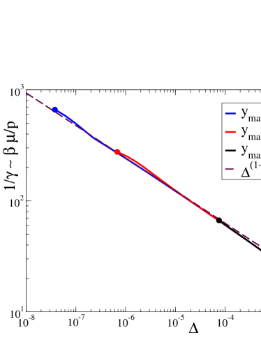
Figure 2: (Left) Schematic evolution of the shear modulus $\mu(t,t_{w})$ and the mean square displacement $\Delta(t,t_{w})$, for a large time $t_{w}$ after a quench, as a function of $t-t_{w}$. (Right) The function $\frac{\beta\widehat{\mu}(\Delta)}{p}\sim 1/\gamma(\Delta)$ that characterizes the reparametrization invariant regime, obtained from the numerical solution of the fullRSB equations Charbonneau et al. (2013). The dots mark the intra-state point $(\widehat{\Delta}_{\rm EA},\beta\widehat{\mu}_{\rm EA}/p)$. The three curves correspond to different cutoffs $y_{\rm max}\propto p$. The slight bending of the curves around the dots is an artifact of the numerical computation Charbonneau et al. (2013).

A more stringent test of the theory can be performed by looking at the so-called reparametrization invariant regime of the out-of-equilibrium dynamics after a quench. Suppose that we perform the aging experiment described above, and starting from a time $t_{w}$ after the quench, we measure both the mean square displacement $\Delta(t,t_{w})=N^{-1}\sum_{i}\langle[x_{i}(t)-x_{i}(t_{w})]^{2}\rangle$ and the shear modulus $\mu(t,t_{w})$. After a short transient, both quantities reach their asymptotic values inside a glass basin, hence $\Delta(t,t_{w})\sim\widehat{\Delta}_{\rm EA}$ and $\mu(t,t_{w})\sim\widehat{\mu}_{\rm EA}$. For large $t_{w}$, and at larger times $t\sim\tau_{\rm mb}(t_{w})$, the dynamics enter in a reparametrization invariant regime Cugliandolo and Kurchan (1994). In this regime, larger and larger groups of states are explored in a restricted equilibrium. Hence, $\Delta(t,t_{w})\sim\Delta(y)$ and $\mu(t,t_{w})\sim\widehat{\mu}(y)$ with the same value of $y$ that is dynamically selected. One can then eliminate time $t$ parametrically from the dynamical data to obtain a curve $\widehat{\mu}(\Delta,t_{w})$. The same can be done in the replica result by eliminating $y$ parametrically to obtain a curve $\widehat{\mu}(\Delta)$. Based on general results obtained in the context of spin glasses Cugliandolo and Kurchan (1994), one expects that

$$\lim_{t_{w}\rightarrow\infty}\widehat{\mu}(\Delta,t_{w})=\widehat{\mu}(\Delta)\ ,$$ (53)

provided in the replica calculation the parameter $m$ is selected to be on the threshold line Cugliandolo and Kurchan (1994); Charbonneau et al. (2013) corresponding to the pressure at which the dynamics is investigated.

The replica prediction is that

$$\frac{\beta\widehat{\mu}(\Delta)}{p}\propto\beta m\widehat{\mu}(\Delta)=\frac{1}{\gamma(\Delta)}\ ,$$ (54)

and because $\Delta(y)\sim y^{-\kappa}$ and $\gamma(y)\sim y^{-\kappa+1}$ for $y\rightarrow\infty$, we have that for $\Delta\rightarrow 0$, $\frac{\beta\widehat{\mu}(\Delta)}{p}\sim 1/\gamma(\Delta)\sim\Delta^{(1-\kappa)/\kappa}$. In other words, in the jamming limit $p\rightarrow\infty$, $\beta\widehat{\mu}(\Delta)$ is proportional to reduced pressure, in such a way that $\frac{\beta\widehat{\mu}(\Delta)}{p}$ tends to a finite limit function. At finite pressure, this master function is defined in an interval $\Delta\in[\widehat{\Delta}_{\rm EA},\widehat{\Delta}_{1}]$. For large pressures, $\widehat{\Delta}_{\rm EA}\sim p^{-\kappa}$ goes to zero, while $\widehat{\Delta}_{1}$ stays finite. Correspondingly the shorter time plateau of the shear modulus diverges faster than $p$, leading to the divergent behavior of the master function, $\frac{\beta\widehat{\mu}(\Delta)}{p}\sim\Delta^{(1-\kappa)/\kappa}$. An illustrative example, obtained from the numerical data of Charbonneau et al. (2013) for $\gamma(y)$ and $\Delta(y)$, is given in Fig. 2.

V Conclusions

By means of the exact solution of amorphous infinite-dimensional hard spheres Kurchan et al. (2012, 2013); Charbonneau et al. (2013), we are able to compute the shear modulus in the whole phase diagram. We found that in $d\rightarrow\infty$ the intra-state shear modulus is simply given by Eq. (48), $\widehat{\mu}_{\rm EA}=T/\widehat{\Delta}_{\rm EA}$ and is equal to temperature divided by the cage radius of the glass. This formula predicts that, at the dynamical transition, $\widehat{\mu}_{\rm EA}$ jumps from zero to a finite value, followed by a square-root singularity, according to Eq. (47). Moreover, it predicts that around the jamming transition $\widehat{\mu}_{\rm EA}$ has critical scalings, described in Sec. IV.2, with critical exponents that are predicted analytically Charbonneau et al. (2013).

Although our results have been obtained in the limit of $d\rightarrow\infty$, which is the only case where an exact solution is possible, they agree with previous analytical results obtained using MCT Fuchs and Cates (2002); Szamel and Flenner (2011), replicas Yoshino (2012, 2013) and effective medium DeGiuli et al. (2014b, a) approaches. We are able to unify these different approaches and put them on a firm theoretical basis, thanks to the fact that the method is exact for $d\rightarrow\infty$. Moreover, our predictions are qualitatively consistent with the most recent and detailed numerical investigations Ikeda et al. (2012). Hence, we believe that our results provide a comprehensive picture of the rheology of complex amorphous fluids.

We also analyzed the behavior of the inter-state shear moduli, that characterize the behavior of the system in situations where it is not confined in a single glass basin, but can also explore neighboring states within larger metabasins. This can happen for example during the out-of-equilibrium dynamics after a sudden deep quench. An interesting result is that the inter-state shear modulus has a different scaling with pressure on approaching jamming, $\beta\widehat{\mu}(y)\sim p\ll p^{\kappa}\sim\beta\widehat{\mu}_{\rm EA}$. This means that if the system is able to explore a little bit of phase space beyond a single glass basin, its rigidity is decreased dramatically. This effect, which is a new prediction, could be detected in numerical simulations and experiments Okamura and Yoshino (2013). We have also discussed the possibility of constructing reparametrization-invariant parametric plots of different observables Cugliandolo and Kurchan (1994), a procedure that should allow one to probe the fullRSB structure of the states close to jamming. Finally, let us recall that the notions of basins and metabasins were proposed within the energy landscape picture of structural glasses Heuer (2008), which naturally implies a hierarchy of rigidities Yoshino (2012).

There are several points that should be discussed further. First of all, this approach can be extended to finite dimensional systems under a mean-field approximation Mezard and Parisi (2012); Parisi and Zamponi (2010); Yoshino (2012). In that case the method is of course approximate, but the qualitative picture (including the scaling properties) is unchanged and the method provides good quantitative estimates of physical observables, the equation of state of the glass Mezard and Parisi (2012); Parisi and Zamponi (2010) and the different transition densities or temperatures. This will be useful to perform more direct comparisons between the theory and numerical simulations Ikeda et al. (2012) or experiments Mason et al. (1997); Klix et al. (2012). Most importantly, the exponent $\nu$ that characterises harmonic soft spheres at zero temperature should be computed, to check whether the predictions of the present approach are consistent with an effective medium computation Wyart (2005); DeGiuli et al. (2014b, a). Of course, most of the conclusions of Ref. Charbonneau et al. (2013) about the fullRSB solution (e.g. how it is affected by critical fluctuations in finite dimensions) also apply to the present work.

Appendix A Fluctuation formula for the shear modulus

A.1 Fluctuation formula

In this section we provide an alternative derivation of Eq. (15) based on the fluctuation formula for the shear modulus matrix that has been derived in Yoshino (2012) and reads

$$N\mu_{ab}=\sum_{i<j}\langle\mu^{a}_{ij}\rangle\delta_{ab}-\beta\left(\sum_{i<j,k<l}\langle\sigma_{ij}^{a}\sigma_{kl}^{b}\rangle-\langle\sigma_{ij}^{a}\rangle\langle\sigma_{kl}^{b}\rangle\right)\ ,$$ (55)

where indexes $i,j,k,l=1,\cdots,N$ run over the molecules of the system, the averages are weighted by the Boltzmann distribution of the molecular liquid and

$$\begin{split}\mu_{ij}^{a}=\mu^{a}(x_{ai}-x_{aj})&=\left.\frac{\partial^{2}}{\partial\gamma_{a}^{2}}v(|S(\gamma_{a})(x_{ai}-x_{aj})|)\right|_{\gamma_{a}=0}\ ,\\ \sigma_{ij}^{a}=\sigma^{a}(x_{ai}-x_{aj})&=\left.\frac{\partial}{\partial\gamma_{a}}v(|S(\gamma_{a})(x_{ai}-x_{aj})|)\right|_{\gamma_{a}=0}\ .\end{split}$$ (56)

This formula can be derived by considering the molecular liquid in the canonical ensemble, without introducing the density field $\rho({\overline{x}})$, and taking the second derivative with respect to shear.

We now introduce a molecular version of the usual $n$-point density functions Hansen and McDonald (1986), which are defined as

$$\rho^{(n)}({\overline{x}}_{1}\cdots{\overline{x}}_{n})=\sum_{i_{1}\neq i_{2}\neq\cdots\neq i_{n}}\langle\delta({\overline{x}}_{i_{1}}-{\overline{x}}_{1})\cdots\delta({\overline{x}}_{i_{n}}-{\overline{x}}_{n})\rangle\ ,$$ (57)

and give the probability of finding $n$ molecules in positions ${\overline{x}}_{1}\cdots{\overline{x}}_{n}$. In terms of these objects, and introducing functions $\mu^{a}({\overline{x}},{\overline{y}})=\mu^{a}(x_{a}-y_{a})$ and $\sigma^{a}({\overline{x}},{\overline{y}})=\sigma^{a}(x_{a}-y_{a})$, we have, as in standard liquid theory Hansen and McDonald (1986):

$$\begin{split}\sum_{i<j}\langle\mu^{a}_{ij}\rangle=&\frac{1}{2}\int d{\overline{x}}d{\overline{y}}\rho^{(2)}({\overline{x}},{\overline{y}})\mu^{a}({\overline{x}},{\overline{y}})\ ,\\ \sum_{i<j}\langle\sigma^{a}_{ij}\rangle=&\frac{1}{2}\int d{\overline{x}}d{\overline{y}}\rho^{(2)}({\overline{x}},{\overline{y}})\sigma^{a}({\overline{x}},{\overline{y}})\ ,\\ \sum_{i<j,k<l}\langle\sigma_{ij}^{a}\sigma_{kl}^{b}\rangle=&\frac{1}{2}\int d{\overline{x}}d{\overline{y}}\rho^{(2)}({\overline{x}},{\overline{y}})\sigma^{a}({\overline{x}},{\overline{y}})\sigma^{b}({\overline{x}},{\overline{y}})\\ &+\int d{\overline{x}}_{1}d{\overline{x}}_{2}d{\overline{x}}_{3}\rho^{(3)}({\overline{x}}_{1},{\overline{x}}_{2},{\overline{x}}_{3})\sigma^{a}({\overline{x}}_{1},{\overline{x}}_{2})\sigma^{b}({\overline{x}}_{1},{\overline{x}}_{3})\\ &+\frac{1}{4}\int d{\overline{x}}_{1}d{\overline{x}}_{2}d{\overline{x}}_{3}d{\overline{x}}_{4}\rho^{(4)}({\overline{x}}_{1},{\overline{x}}_{2},{\overline{x}}_{3},{\overline{x}}_{4})\sigma^{a}({\overline{x}}_{1},{\overline{x}}_{2})\sigma^{b}({\overline{x}}_{3},{\overline{x}}_{4})\ .\end{split}$$ (58)

We now make use of the fact that, according to the analysis of Frisch and Percus (1999); Torquato and Stillinger (2006) in the limit $d\rightarrow\infty$, many-body correlations factor in products of two body correlations, and moreover the two-body correlation is given by its first virial contribution. Equivalently one can say that all $n$-point functions are given by their lowest order virial contribution, which is Salpeter (1958):

$$\rho^{(n)}({\overline{x}}_{1}\cdots{\overline{x}}_{n})=\prod_{i=1}^{n}\rho({\overline{x}}_{i})\prod_{i<j}^{1,n}e^{-\beta v({\overline{x}}_{i},{\overline{x}}_{j})}\ ,$$ (59)

where

$$e^{-\beta v({\overline{x}},{\overline{y}})}=\prod_{a=1}^{m}e^{-\beta v(x_{a}-y_{a})}$$ (60)

is the replicated interaction potential.

Using this, we get

$$\begin{split}N\mu_{ab}=&\frac{1}{2}\int d{\overline{x}}d{\overline{y}}\rho({\overline{x}})\rho({\overline{y}})e^{-\beta v({\overline{x}},{\overline{y}})}[\mu^{a}({\overline{x}},{\overline{y}})\delta_{ab}-\beta\sigma^{a}({\overline{x}},{\overline{y}})\sigma^{b}({\overline{x}},{\overline{y}})]\\ &-\beta\int d{\overline{x}}_{1}d{\overline{x}}_{2}d{\overline{x}}_{3}\rho({\overline{x}}_{1})\rho({\overline{x}}_{2})\rho({\overline{x}}_{3})e^{-\beta v({\overline{x}}_{1},{\overline{x}}_{2})}e^{-\beta v({\overline{x}}_{2},{\overline{x}}_{3})}e^{-\beta v({\overline{x}}_{3},{\overline{x}}_{1})}\sigma^{a}({\overline{x}}_{1},{\overline{x}}_{2})\sigma^{b}({\overline{x}}_{1},{\overline{x}}_{3})\\ &-\frac{\beta}{4}\int d{\overline{x}}_{1}d{\overline{x}}_{2}d{\overline{x}}_{3}d{\overline{x}}_{4}\prod_{i=1}^{4}\rho({\overline{x}}_{i})\left[\prod_{i<j}^{1,4}e^{-\beta v({\overline{x}}_{i},{\overline{x}}_{j})}-e^{-\beta v({\overline{x}}_{1},{\overline{x}}_{2})}e^{-\beta v({\overline{x}}_{3},{\overline{x}}_{4})}\right]\sigma^{a}({\overline{x}}_{1},{\overline{x}}_{2})\sigma^{b}({\overline{x}}_{3},{\overline{x}}_{4})\end{split}$$ (61)

It is easy to show that the last two lines of the previous equation vanish in $d\rightarrow\infty$. Consider for example the three-body term. The integral is dominated by configurations where ${\overline{x}}_{1}-{\overline{x}}_{2}\sim D$ is orthogonal to ${\overline{x}}_{1}-{\overline{x}}_{3}\sim D$, so that ${\overline{x}}_{1}$ and ${\overline{x}}_{3}$ are far away and $e^{-\beta v({\overline{x}}_{3},{\overline{x}}_{1})}\sim 1$ and can be neglected. The remaining integral can be evaluated through a saddle point and to leading order it is equal to the square of the average of $\sigma^{a}$, which vanishes in an isotropic liquid. Similarly, the last line is dominated by configurations where e.g. 1 and 3 overlap, 1 and 2 (and 3 and 4) are at distance $\sim D$, and 2 and 4 are far away. Again at this leading order one obtains the square of the average of $\sigma^{a}$, which vanishes. This analysis is consistent with the general principle that all contributions to thermodynamic averages coming from $n$-body correlation for $n>2$ vanish in high dimensions Torquato and Stillinger (2006). Since the only two body contribution in the second and third line of Eq. (61) is the average of $\sigma^{a}$ which is zero,  these contributions must vanish.

We obtain

$$\mu_{ab}=\frac{1}{2N}\int d{\overline{x}}d{\overline{y}}\rho({\overline{x}})\rho({\overline{y}})e^{-\beta v({\overline{x}},{\overline{y}})}[\mu^{a}({\overline{x}},{\overline{y}})\delta_{ab}-\beta\sigma^{a}({\overline{x}},{\overline{y}})\sigma^{b}({\overline{x}},{\overline{y}})]\ ,$$ (62)

and inserting the explicit expressions of $\mu^{a}$ and $\sigma^{a}$ it is easy to check that this expression becomes

$$\beta\mu_{ab}=-\frac{1}{2N}\int d\overline{x}d\overline{y}\rho(\overline{x})\rho(\overline{y})(x_{a2}-y_{a2})(x_{b2}-y_{b2})\frac{\partial^{2}f}{\partial x_{a1}\partial x_{b1}}(\overline{x}-\overline{y})\ ,$$ (63)

where $f$ is the usual replicated Mayer function in absence of shear-strain Kurchan et al. (2012), corresponding to Eq. (4) for $\gamma_{a}=0$. We now take into account translational invariance following the discussion of Kurchan et al. (2012). We introduce coordinates $u_{a}=x_{a}-X$ with $X=m^{-1}\sum_{a}x_{a}$, and we use that $\rho(\overline{x})$ does not depend on $X$, to obtain, following the notations of Kurchan et al. (2012):

$$\beta\mu_{ab}=-\frac{1}{2\rho}\int dX{\cal D}\overline{u}{\cal D}\overline{v}\rho(\overline{u})\rho(\overline{v})(X_{2}+u_{a2}-v_{a2})(X_{2}+u_{b2}-v_{b2})\frac{\partial^{2}f}{\partial u_{a1}\partial u_{b1}}(X+\overline{u}-\overline{v})\ .$$ (64)

A.2 Simplifications for $d\rightarrow\infty$

We now make use of the results of (Kurchan et al., 2012, Sec. 5), that show that the integral in Eq. (64) is dominated by the region where $u_{a}\sim v_{a}\sim d^{-1/2}$, while $X$ is decomposed in a $(d-m)$-component vector $X_{\perp}$, orthogonal to the plane defined by $\overline{u}-\overline{v}$, that is of order $D$, and a $m$-component vector $X_{\parallel}\sim d^{-1/2}$. This structure allows us to perform a series of crucial simplifications of Eq. (64). It is clear, in fact, that with probability going to 1 for $d\rightarrow\infty$ with respect to the random choice of $\overline{u},\overline{v}$ according to the probability density $\rho(\overline{u})\rho(\overline{v})$, the direction $\mu=2$ is orthogonal to all the vectors $u_{a}$ and $v_{a}$, and therefore we can neglect the terms $u_{a2}$ and $v_{a2}$ in Eq. (64). This is further supported by the fact that the vectors $u_{a}$ and $v_{a}$ are small in the limit $d\rightarrow\infty$ while $X=X_{\perp}+X_{\parallel}$ remains of order 1 in most directions. We therefore obtain

$$\beta\mu_{ab}=-\frac{1}{2\rho}\int{\cal D}\overline{u}{\cal D}\overline{v}\rho(\overline{u})\rho(\overline{v})\frac{\partial^{2}}{\partial u_{a1}\partial u_{b1}}\int dX(X_{2})^{2}f(X+\overline{u}-\overline{v})$$ (65)

We now observe that direction $\mu=2$ is equivalent to any other direction $\mu>1$, because the shear-strain has been eliminated and we are now considering an isotropic system. Direction $\mu=1$ is still special due to the presence of the derivative, but we can consider this as a $1/d$ correction, therefore we can write

$$\beta\mu_{ab}=-\frac{1}{2\rho}\int{\cal D}\overline{u}{\cal D}\overline{v}\rho(\overline{u})\rho(\overline{v})\frac{\partial^{2}}{\partial u_{a1}\partial u_{b1}}\frac{1}{d}\int dXX^{2}f(X+\overline{u}-\overline{v})\ ,$$ (66)

and, recalling once again that $X=X_{\perp}+X_{\parallel}$ with $X_{\perp}\sim D$ and $X_{\parallel}\sim d^{-1/2}$, we have at leading order

$$\beta\mu_{ab}=-\frac{1}{2\rho}\int{\cal D}\overline{u}{\cal D}\overline{v}\rho(\overline{u})\rho(\overline{v})\frac{\partial^{2}}{\partial u_{a1}\partial u_{b1}}\frac{1}{d}\int dXX_{\perp}^{2}f(X+\overline{u}-\overline{v})\ ,$$ (67)

Now we specialize to the case of hard spheres, and following exactly the same steps of (Kurchan et al., 2012, Sec. 5, Eqs.(31)-(33)), we obtain

$$\int dXX_{\perp}^{2}f(X+\overline{u})=-V_{d}D^{d}\,\frac{\int d^{m}X_{\parallel}\,\Theta_{d-m+2}(D^{2}-\min_{a}|X_{\parallel}+u_{a}|^{2})}{\int d^{m}X_{\parallel}\,\Theta_{d-m}(D^{2}-|X_{\parallel}|^{2})}\ .$$ (68)

Next, following the steps of (Kurchan et al., 2012, Sec. 5.2), and introducing $x_{a}$ by $u_{a}=x_{a}D/\sqrt{d}$, we obtain

$$\int dXX_{\perp}^{2}f(X+\overline{u})=-V_{d}D^{d+2}\ \frac{\int d^{m}\epsilon\,e^{-\frac{1}{2}\min_{a}|\epsilon+x_{a}|^{2}}}{\int d^{m}\epsilon\,e^{-\frac{1}{2}|\epsilon|^{2}}}=-V_{d}D^{d+2}{\cal F}(\overline{x})=-V_{d}D^{d+2}{\cal F}\left(\frac{\sqrt{d}}{D}\,\overline{u}\right)\ ,$$ (69)

and

$$\beta\mu_{ab}=\frac{V_{d}D^{d+2}}{2\rho\,d}\int{\cal D}\overline{u}{\cal D}\overline{v}\rho(\overline{u})\rho(\overline{v})\frac{\partial^{2}}{\partial u_{a1}\partial u_{b1}}{\cal F}\left(\frac{\sqrt{d}}{D}\,(\overline{u}-\overline{v})\right)\ .$$ (70)

A.3 Saddle point evaluation

It has been shown in Kurchan et al. (2012) that for $d\rightarrow\infty$, integrals such as (70) are dominated by a saddle point on $\overline{u}$ and $\overline{v}$, due to the fact that $\rho(\overline{u})$ is exponential in $d$. Because the function ${\cal F}$ is not exponential in $d$, it does not contribute to the saddle point. Because $\int{\cal D}\overline{u}\rho(\overline{u})=\rho$, we obtain, recalling that $\rho V_{d}D^{d}=2^{d}\varphi=d\widehat{\varphi}$ where $\varphi$ is the packing fraction and $\widehat{\varphi}$ a scaled packing fraction,

$$\beta\mu_{ab}=\frac{\rho V_{d}D^{d+2}}{2d}\frac{\partial^{2}}{\partial u_{a1}\partial u_{b1}}{\cal F}\left(\frac{\sqrt{d}}{D}\,(\overline{u}^{\rm sp}-\overline{v}^{\rm sp})\right)=\frac{\widehat{\varphi}D^{2}}{2}\frac{\partial^{2}}{\partial u_{a1}\partial u_{b1}}{\cal F}\left(\frac{\sqrt{d}}{D}\,(\overline{u}^{\rm sp}-\overline{v}^{\rm sp})\right)\ .$$ (71)

The function ${\cal F}$ is rotationally invariant, hence it depends only on $(u_{a}-v_{a})\cdot(u_{b}-v_{b})$. We can choose any values of $\overline{u}^{\rm sp}$ and $\overline{v}^{\rm sp}$, provided they respect the saddle point equations, which state Kurchan et al. (2012) that $u_{a}\cdot u_{b}=q_{ab}$, $v_{a}\cdot v_{b}=p_{ab}$, and $u_{a}\cdot v_{b}=0$, hence $(u_{a}-v_{a})\cdot(u_{b}-v_{b})=q_{ab}+p_{ab}$. We have that $\hat{q}=\hat{p}$, however when we take the derivative with respect to $u_{a}$ we should only differentiate with respect to $\hat{q}$ and not to $\hat{p}$. We can simplify this by writing

$$\beta\mu_{ab}=\frac{\widehat{\varphi}D^{2}}{2}\left.\frac{\partial^{2}}{\partial u_{a1}\partial u_{b1}}{\cal F}\left(\frac{d}{D^{2}}\,(\hat{q}_{ab}+\hat{p}_{ab})\right)\right|_{\hat{p}=\hat{q}}=\frac{\widehat{\varphi}D^{2}}{4}\frac{\partial^{2}}{\partial u_{a1}\partial u_{b1}}{\cal F}\left(2\frac{d}{D^{2}}\,\hat{q}_{ab}\right)\ .$$ (72)

Also, following Kurchan et al. (2013); Charbonneau et al. (2013) we can introduce the matrix

$$\Delta_{ab}=\frac{d}{D^{2}}(u_{a}-u_{b})^{2}=\frac{d}{D^{2}}(q_{aa}+q_{bb}-2q_{ab})\ ,$$ (73)

and we have, following the definitions of Charbonneau et al. (2013), that

$$\beta\mu_{ab}=\frac{\widehat{\varphi}D^{2}}{4}\frac{\partial^{2}}{\partial u_{a1}\partial u_{b1}}{\cal F}(\hat{\Delta})\ ,$$ (74)

with ${\cal F}(\hat{\Delta})$ given in Charbonneau et al. (2013). We have then

$$\frac{\partial}{\partial u_{a1}}{\cal F}(\hat{\Delta})=\frac{d}{D^{2}}\sum_{c(\neq a)}2(u_{a1}-u_{c1})\frac{\partial{\cal F}}{\partial\Delta_{ac}}\ ,$$ (75)

and

$$\frac{\partial^{2}}{\partial u_{a1}\partial u_{b1}}{\cal F}(\hat{\Delta})=\frac{d}{D^{2}}\times\begin{cases}2\sum_{c(\neq a)}\frac{\partial{\cal F}}{\partial\Delta_{ac}}+\sum_{c(\neq a),d(\neq a)}\frac{\partial^{2}{\cal F}}{\partial\Delta_{ac}\partial\Delta_{ad}}4\frac{d}{D^{2}}(u_{a1}-u_{c1})(u_{a1}-u_{d1})&\text{for }a=b\\ -2\frac{\partial{\cal F}}{\partial\Delta_{ab}}+\sum_{c(\neq a),d(\neq b)}\frac{\partial^{2}{\cal F}}{\partial\Delta_{ac}\partial\Delta_{bd}}4\frac{d}{D^{2}}(u_{a1}-u_{c1})(u_{b1}-u_{d1})&\text{for }a\neq b\\ \end{cases}$$ (76)

In each line of the previous equation, the second term is a factor $1/d$ smaller than the first, because it contains terms like $\frac{d}{D^{2}}u_{a1}^{2}=\frac{d}{D^{2}}q_{aa}/d\propto\Delta/d$, hence it can be neglected. We obtain

$$\frac{\partial^{2}}{\partial u_{a1}\partial u_{b1}}{\cal F}(\hat{\Delta})=\frac{2d}{D^{2}}\left[\delta_{ab}\sum_{c(\neq a)}\frac{\partial{\cal F}}{\partial\Delta_{ac}}-(1-\delta_{ab})\frac{\partial{\cal F}}{\partial\Delta_{ab}}\right]\ ,$$ (77)

and using this we obtain our final result

$$\beta\mu_{ab}=\frac{d}{2}\,\widehat{\varphi}\left[\delta_{ab}\sum_{c(\neq a)}\frac{\partial{\cal F}}{\partial\Delta_{ac}}-(1-\delta_{ab})\frac{\partial{\cal F}}{\partial\Delta_{ab}}\right]\ ,$$ (78)

which coincides with Eq. (15).

References

- Torquato and Stillinger (2010) S. Torquato and F. H. Stillinger, Rev. Mod. Phys. 82, 2633 (2010).
- Parisi and Zamponi (2010) G. Parisi and F. Zamponi, Rev. Mod. Phys. 82, 789 (2010).
- Berthier and Biroli (2011) L. Berthier and G. Biroli, Rev. Mod. Phys. 83, 587 (2011).
- Ikeda et al. (2012) A. Ikeda, L. Berthier, and P. Sollich, Phys. Rev. Lett. 109, 018301 (2012).
- Szamel and Flenner (2011) G. Szamel and E. Flenner, Physical review letters 107, 105505 (2011).
- Yoshino (2012) H. Yoshino, The Journal of Chemical Physics 136, 214108 (2012).
- Fuchs and Cates (2002) M. Fuchs and M. E. Cates, Physical Review Letters 89, 248304 (2002).
- Mason and Weitz (1995) T. Mason and D. Weitz, Physical review letters 75, 2770 (1995).
- Brito and Wyart (2006) C. Brito and M. Wyart, Europhysics Letters (EPL) 76, 149 (2006).
- Pusey and Van Megen (1986) P. Pusey and W. Van Megen, Nature 320, 340 (1986).
- Bernal and Mason (1960) J. Bernal and J. Mason, Nature 188, 910 (1960).
- Liu et al. (2011) A. Liu, S. Nagel, W. Van Saarloos, and M. Wyart, in Dynamical Heterogeneities and Glasses, edited by L. Berthier, G. Biroli, J.-P. Bouchaud, L. Cipelletti, and W. van Saarloos (Oxford University Press, 2011), eprint arXiv:1006.2365.
- O’Hern et al. (2002) C. S. O’Hern, S. A. Langer, A. J. Liu, and S. R. Nagel, Phys. Rev. Lett. 88, 075507 (2002).
- Mason et al. (1997) T. G. Mason, M.-D. Lacasse, G. S. Grest, D. Levine, J. Bibette, and D. A. Weitz, Phys. Rev. E 56, 3150 (1997).
- Ikeda et al. (2013) A. Ikeda, L. Berthier, and G. Biroli, J. Chem. Phys. 138, 12A507 (2013).
- Berthier and Witten (2009) L. Berthier and T. A. Witten, Phys. Rev. E 80, 021502 (2009).
- Berthier et al. (2011) L. Berthier, H. Jacquin, and F. Zamponi, Phys. Rev. E 84, 051103 (2011).
- Yoshino (2013) H. Yoshino, AIP Conference Proceedings 1518, 244 (2013), eprint arXiv:1210.6826.
- Zaccone and Scossa-Romano (2011) A. Zaccone and E. Scossa-Romano, Phys. Rev. B 83, 184205 (2011).
- Wyart (2005) M. Wyart, Annales de Physique 30, 1 (2005), eprint arXiv:cond-mat/0512155.
- DeGiuli et al. (2014a) E. DeGiuli, E. Lerner, C. Brito, and M. Wyart, arXiv:1402.3834 (2014a).
- DeGiuli et al. (2014b) E. DeGiuli, A. Laversanne-Finot, G. Düring, E. Lerner, and M. Wyart, arXiv:1401.6563 (2014b).
- Charbonneau et al. (2012) P. Charbonneau, E. I. Corwin, G. Parisi, and F. Zamponi, Phys. Rev. Lett. 109, 205501 (2012).
- Lerner et al. (2013) E. Lerner, G. During, and M. Wyart, Soft Matter 9, 8252 (2013).
- Götze (2009) W. Götze, Complex dynamics of glass-forming liquids: A mode-coupling theory, vol. 143 (Oxford University Press, USA, 2009).
- Ikeda and Berthier (2013) A. Ikeda and L. Berthier, Phys. Rev. E 88, 052305 (2013).
- Mezard and Parisi (2012) M. Mezard and G. Parisi, in Structural Glasses and Supercooled Liquids: Theory, Experiment and Applications, edited by P.G.Wolynes and V.Lubchenko (Wiley & Sons, 2012), eprint arXiv:0910.2838.
- Yoshino and Mézard (2010) H. Yoshino and M. Mézard, Phys. Rev. Lett. 105, 015504 (2010).
- Okamura and Yoshino (2013) S. Okamura and H. Yoshino, arXiv:1306.2777 (2013).
- Kirkpatrick and Wolynes (1987) T. R. Kirkpatrick and P. G. Wolynes, Phys. Rev. A 35, 3072 (1987).
- Kirkpatrick and Thirumalai (1987) T. R. Kirkpatrick and D. Thirumalai, Phys. Rev. Lett. 58, 2091 (1987).
- Kirkpatrick et al. (1989) T. R. Kirkpatrick, D. Thirumalai, and P. G. Wolynes, Phys. Rev. A 40, 1045 (1989).
- Witten (1980) E. Witten, Physics Today 33, 38 (1980).
- Kurchan et al. (2012) J. Kurchan, G. Parisi, and F. Zamponi, Journal of Statistical Mechanics: Theory and Experiment 2012, P10012 (2012).
- Kurchan et al. (2013) J. Kurchan, G. Parisi, P. Urbani, and F. Zamponi, J. Phys. Chem. B 117, 12979 (2013).
- Charbonneau et al. (2013) P. Charbonneau, J. Kurchan, G. Parisi, P. Urbani, and F. Zamponi, arXiv:1310.2549 (2013).
- Charbonneau et al. (2014) P. Charbonneau, J. Kurchan, G. Parisi, P. Urbani, and F. Zamponi, Nature Communications 5, 3725 (2014).
- Gardner (1985) E. Gardner, Nuclear Physics B 257, 747 (1985).
- Mézard et al. (1987) M. Mézard, G. Parisi, and M. A. Virasoro, Spin glass theory and beyond (World Scientific, Singapore, 1987).
- Charbonneau et al. (2011) P. Charbonneau, A. Ikeda, G. Parisi, and F. Zamponi, Phys. Rev. Lett. 107, 185702 (2011).
- Castellani and Cavagna (2005) T. Castellani and A. Cavagna, Journal of Statistical Mechanics: Theory and Experiment 2005, P05012 (2005).
- Monasson (1995) R. Monasson, Phys. Rev. Lett. 75, 2847 (1995).
- Mézard and Parisi (1996) M. Mézard and G. Parisi, Journal of Physics A: Mathematical and General 29, 6515 (1996).
- Frisch and Percus (1999) H. L. Frisch and J. K. Percus, Phys. Rev. E 60, 2942 (1999).
- Klix et al. (2012) C. L. Klix, F. Ebert, F. Weysser, M. Fuchs, G. Maret, and P. Keim, Phys. Rev. Lett. 109, 178301 (2012).
- Cugliandolo and Kurchan (1994) L. F. Cugliandolo and J. Kurchan, Journal of Physics A: Mathematical and General 27, 5749 (1994).
- Yeo and Moore (2012) J. Yeo and M. A. Moore, Phys. Rev. E 86, 052501 (2012).
- Fullerton and Moore (2013) C. J. Fullerton and M. Moore, arXiv:1304.4420 (2013).
- Franz and Parisi (2013) S. Franz and G. Parisi, Journal of Statistical Mechanics: Theory and Experiment 2013, P11012 (2013).
- Biroli et al. (2013) G. Biroli, C. Cammarota, G. Tarjus, and M. Tarzia, arXiv:1309.3194 (2013).
- (51) G. Biroli and P. Urbani, in preparation.
- Rizzo (2013) T. Rizzo, Phys. Rev. E 88, 032135 (2013).
- Heuer (2008) A. Heuer, Journal of Physics: Condensed Matter 20, 373101 (2008).
- Hansen and McDonald (1986) J.-P. Hansen and I. R. McDonald, Theory of simple liquids (Academic Press, London, 1986).
- Torquato and Stillinger (2006) S. Torquato and F. H. Stillinger, Experimental Mathematics 15, 307 (2006).
- Salpeter (1958) E. E. Salpeter, Annals of Physics 5, 183 (1958).