Representation and Network Synthesis for a Class of Mixed Quantum-Classical Linear Stochastic Systems

Abstract

The purpose of this paper is to present a network realization theory for a class of mixed quantum-classical linear stochastic systems. Two forms, the standard form and the general form, of this class of linear mixed quantum-classical systems are proposed. Necessary and sufficient conditions for their physical realizability are derived. Based on these physical realizability conditions, a network synthesis theory for this class of linear mixed quantum-classical systems is developed, which clearly exhibits the quantum component, the classical component, and their interface. An example is used to illustrate the theory presented in this paper.

Index Terms— linear stochastic systems, mixed quantum-classical linear stochastic systems, quantum systems, classical probability, quantum probability, network synthesis theory, physical realizability condition.

I Introduction

Linear systems are of basic importance to classical control engineering, and also arise in the modeling and control of quantum systems; see, e.g., [14], [1], [28], [15], [36], [41], [11], [48], [49], [4], [22], [19], [44], [50], [45], [32], [51]. A classical linear system described by the state space representation can be realized using electrical components by linear electrical network synthesis theory, see [2]. Linear quantum optical systems may be described by linear quantum differential equations in the Heisenberg picture of quantum mechanics, [14], [23], [29], [41], [15], [43], [19], [44], [32], [51]. Such quantum linear systems described by the state space representation can be built by optical cavities, degenerate parametric amplifiers (DPA), phase shifters, beam splitters, and squeezers, etc; interested readers may refer to [25], [5], [30], [32] for a more detailed introduction to these optical devices. Quantum technologies often comprise quantum systems interconnected with classical (non-quantum) devices, which means that the two types of systems may be connected as an integral whole (called mixed quantum-classical systems in this paper) by appropriate interfaces that convert quantum signals to classical signals, and vice-versa. Traditionally, such quantum optical networks would be implemented on an optical table. However, it is now becoming possible to consider implementation in semiconductor chips, [7], [35], [43].

In classical control engineering, many methods have been developed for designing controllers that meet various control specifications. The design process begins with some form of specification for the system, and concludes with a physical realization of the controller that meets the specifications. Often, mathematical models for the controller are used in the design process, such as state space equations for the controller. These state space equations may result from a mathematical optimization procedure, such as $H^{\infty}$, LQG, or some other procedure. The process of going from such mathematical models to the desired physical systems is a process of synthesis or physical realization, part of the design methodologies widely used in classical engineering [2]. Analogous design issues are beginning to present themselves in quantum technology. A quantum control system often has both quantum and classical components. Indeed, in measurement-based feedback control, a classical controller is used to control a quantum plant. That is, a quantum control system is often a mixed quantum-classical system. Figure 1 illustrates an example of a mixed quantum-classical linear system studied in [36]. In this measurement-based feedback control system, a Fabry-Perot optical cavity [5], [30], [40], which is described quantum-mechanically, is connected to a classical controller via a homodyne detector (HD) and a piezo-electric actuator [41], [39]. The light field (quantum signal) reflected from the cavity is first separated from the incoming laser beam by an optical isolator, and then is detected by a HD (a quantum-to-classical converter), thus yielding a photocurrent which is a classical signal. The classical controller processes such classical signals to generate a classical control input $u$, which is then fed back to regulate the optical path length of the cavity via the piezo-electric actuator in order to actuate the resonant frequency of the cavity. Interested reader may refer to [36] for more details.

The purpose of this paper is to propose canonical representations for a class of linear stochastic differential equations that may describe mixed quantum-classical systems and then develop a network synthesis theory for such class of equations that reveals in a clear way the internal structure of a mixed quantum-classical system. Furthermore, arbitrary linear stochastic differential equations for mixed systems need not correspond to a physical system, and so we derive conditions ensuring that they do; that is, physical realizability. This work generalizes and extends earlier work [23], [31], [42]. In [42], we only consider a standard model for mixed quantum-classical linear stochastic systems for the design process. However, in this paper, we will investigate a more general model for the physical realization of mixed quantum-classical linear stochastic systems.

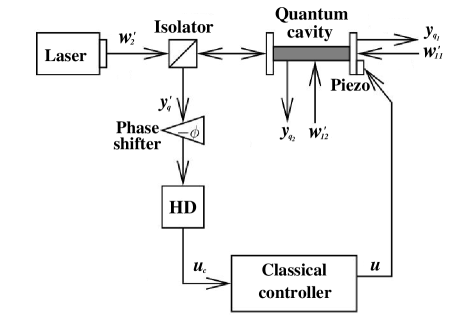
Figure 1: A mixed quantum-classical system (Cavity locking feedback control loop) studied in [36].

The rest of the paper is organized as follows. Section II introduces some concepts about classical and quantum random variables as well as probabilities, briefly describes closed quantum harmonic oscillators, and also gives a brief overview of linear non-commutative stochastic systems and non-demolition conditions. Section III proposes two models of mixed quantum-classical linear stochastic systems for the design process and presents a connection between these models. Section IV presents physical realizability definitions and constraints for the two models defined in Section III, respectively. Section V develops a network synthesis theory for a mixed quantum-classical system. Section VI presents a potential application of the main results of Section V. Finally, Section VII gives the conclusion of this paper.

II Preliminaries

II-A Notation

The notations used in this paper are as follows. The imaginary unit is $i=\sqrt{-1}$. The commutator of two operators $A$ and $B$ is defined by $[A,~{}B]=AB-BA$. If $x$ and $y$ are column vectors of operators, the commutator is defined by $[x,~{}y^{T}]=xy^{T}-(yx^{T})^{T}$. If $X=[x_{jk}]$ is a matrix of linear operators or complex numbers, then $X^{\#}=[x^{*}_{jk}]$ denotes the operation of taking the adjoint of each element of $X$, and $X^{{\dagger}}=[x^{*}_{jk}]^{T}$. We also define $\Re(X)=(X+X^{\#})/2$ and $\Im(X)=(X-X^{\#})/2i$. The symbol $I_{k}$ denotes the $k\times k$ identity matrix, $0_{j\times k}$ denotes the $j\times k$ zero matrix and $0_{k}\equiv 0_{k\times k}$. Let $J=\left[\begin{array}[]{cc}0&1\\ -1&0\\ \end{array}\right]$ and $\mathrm{diag}_{k}(M)$ denote a block diagonal matrix with the square matrix $M$ appearing $k$ times on the diagonal block. A symplectic matrix $V$ of dimension $2k\times 2k$ is a real matrix satisfying $V\Theta_{k}V^{T}=\Theta_{k}$, where $\Theta_{k}={\rm diag}_{k}(J)$. We set $\hbar=1$ throughout this paper.

II-B Classical and quantum random variables

A classical random variable, usually written as $X$, is a variable whose possible values are numerical outcomes of a random phenomenon. A random variable $X$ with mean $\mu=\mathbf{E}[X]$ and variance $\sigma^{2}=\mathbf{E}[(X-\mu)^{2}]$ is said to be Gaussian if its probability distribution function $F$ is Gaussian, i.e.,

$$F(a<X\leq b)=\int_{a}^{b}p_{X}(x)dx,~{}~{}~{}\forall-\infty<a<b<\infty,$$ (1)

where $p_{X}(x)=\frac{1}{\sigma\sqrt{2\pi}}\mathrm{exp}(-\frac{(x-\mu)^{2}}{2\sigma^{2}})$ is of course the well-known Gaussian probability density function.

In quantum physics, a quantum random variable $A$ is an operator defined on a Hilbert space $\mathfrak{H}$. In particular, if $A$ is self-adjoint, it is called an observable and can be used to represent some physical quantity. Because an observable is self-adjoint, by the spectral theory, its spectra are real numbers. Actually, an observable can be physically measured to generate outcomes which are real numbers. On the other hand, a quantum state $\psi$ encodes an experimenter’s knowledge or information about some aspect of reality and is given mathematically as a vector of $\mathfrak{H}$, permitting the calculation of expected values of quantum random variables. If an observable $A$ is measured on a quantum system prepared in the state $\psi$, then its mean value is given by the inner product $\langle\psi,A\psi\rangle=\int_{-\infty}^{\infty}\psi(q)^{*}A\psi(q)dq$. In quantum mechanics, the Dirac “ket” notation $|\psi\rangle$ is always used to denote a pure quantum state $\psi$. The adjoint of $|\psi\rangle$ is the “bra” vector $\langle\psi|$. Then, we can write the previous inner product as $\langle\psi,A\psi\rangle=\langle\psi|A\psi\rangle$. Moreover, we can associate a density operator $\rho$ with state $|\psi\rangle$ as $\rho=|\psi\rangle\langle\psi|$. The density operator $\rho$ defined in this way corresponds to a pure state and is a rank-1 projector, but in general $\rho$ can also be used to describe a classical mixture of pure states, [27, 41].

Consider an example of a quantum harmonic oscillator with amplitude quadrature operator $Q$ and phase quadrature operator $P$, a model for an optical mode in a cavity. The two observables $Q$ and $P$ are defined by

$$(Q\psi)(q)=q\psi(q),\ \ \ (P\psi)(q)=-i\frac{d}{dq}\psi(q)$$ (2)

for $\psi\in\mathfrak{H}=L^{2}(\mathbb{R})$, respectively. In quantum mechanics, the amplitude and phase quadrature observables satisfy the commutation relation $[Q,~{}P]=2i$, and such non-commuting observables are referred to as being incompatible. The state vector

$$\psi(q)=(2\pi)^{-\frac{1}{4}}\sigma^{-\frac{1}{2}}\mathrm{exp}\left(-\frac{(q-\mu)^{2}}{4\sigma^{2}}\right)$$ (3)

is an instance of what is known as a quantum Gaussian state. For this particular Gaussian state, the means of $P$ and $Q$ are given by $\int_{-\infty}^{\infty}\psi(q)^{*}Q\psi(q)dq=\mu$, and $\int_{-\infty}^{\infty}\psi(q)^{*}P\psi(q)dq=0$, and similarly the variances are $\sigma^{2}$ and $\frac{1}{4\sigma^{2}}$, respectively.

II-C Classical probability and quantum probability

In the classical probability theory, a probability model is given by a triple ($\Omega,F,\nu$), where

1. the sample space $\Omega$ is the set of all possible outcomes of some experiment;

2. $F$ is a collection of events, which are subsets of $\Omega$;

3. $\nu$ is a probability measure.

Classical random variables can be defined on the probability space ($\Omega,F,\nu$). For instance, when $\Omega=\mathbb{R}$, $F$ is the $\sigma$-field generated by all the sets of the form $(a,b]$, and probability measure $\nu$ is defined in terms of $p_{X}(x)$ used given in Eq. (1), specifically,

$$\nu(A)=\int_{A}p_{X}(x)dx,~{}~{}~{}\forall A\in F,$$

then the associated random variable $X$ is a Gaussian random variable.

The quantum probability model, a generalization of the classical probability model [3], [20], [6], can be defined at the level of von Neumann algebra and density operators. More specifically, a quantum probability model ($\mathcal{A},\rho$) (also called a quantum probability space) consists of

1. a von Neumann algebra $\mathcal{A}$ generated by a collection of projection operators on a Hilbert space $\mathfrak{H}$ (the projections $E\in\mathcal{A}$ are called events in $\mathcal{A}$);

2. a density operator $\rho$. The trace ${\rm tr}[\rho E]$ gives the probability that an event $E\in\mathcal{A}$ occurs, where events in a quaantum probability space are represented by projection operators.

The quantum probability model is the most natural non-commutative generalization of classical probability, in the sense that every classical probability space can be embedded in a quantum probability space. For example, given a vector of classical Gaussian random variables $\tilde{X}=[X_{1}\quad X_{2}\quad\cdots\quad X_{k}]^{T}$ with joint probability density function

$$f(q)=(2\pi)^{-\frac{k}{2}}|\Sigma|^{-\frac{1}{2}}\mathrm{exp}\left(-\frac{1}{2}(q-\tilde{\mu})^{T}\Sigma^{-1}(q-\tilde{\mu})\right)$$ (4)

with mean $\tilde{\mu}\in\mathbb{R}^{k}$ and covariance matrix $\Sigma\in\mathbb{R}^{k\times k}$, we may define the quantum state $\psi=\sqrt{f(q)}$ and a vector of quantum observables $\check{X}_{Q}=[Q_{1}\quad Q_{2}\quad\cdots\quad Q_{k}]^{T}$ by means of $(Q_{j}\psi)(q)=q_{j}\psi(q)$ for $j=1,\ldots,k$. It is easy to show that the classical Gaussian random variables $\tilde{X}$ and the quantum Gaussian random variables $\check{X}_{Q}$ have the same mean and variance values, thus having the identical distribution. So statistically, $\tilde{X}\equiv\check{X}_{Q}$. In the similar way as in Eq. (2), we may define a vector of quantum observables $\check{X}_{P}=[P_{1}\quad P_{2}\quad\cdots\quad P_{k}]^{T}$ by means of $(P_{j}\psi)(q)=-i\frac{\partial}{\partial q_{j}}\psi(q)$ for $j=1,\ldots,k$. Then it is easy to see that $[\check{X}_{Q},~{}\check{X}_{P}^{T}]=2iI_{k}$. Let $\mathbf{P}\in\mathbb{R}^{2k\times 2k}$ be a permutation matrix such that $\mathbf{P}\check{X}=[Q_{1}\quad P_{1}\quad\cdots\quad Q_{k}\quad P_{k}]^{T}$. Then the commutation relation becomes $[(\mathbf{P}\check{X}),~{}(\mathbf{P}\check{X})^{T}]=2i{\rm diag}_{k}(J)\equiv 2i\Theta_{k}$. The quantum vector $\check{X}=[\check{X}_{Q}^{T}\quad\check{X}_{P}^{T}]^{T}$ is called an augmentation of $\tilde{X}$. The relation between classical and quantum random variables may be expressed as $\tilde{X}\equiv[\begin{array}[]{cc}I_{k}&0_{k}\end{array}]\left[\begin{array}[]{c}\check{X}_{Q}\\ \check{X}_{P}\end{array}\right]$. In the rest of the paper, we use symbol “$=$” instead of “$\equiv$” to represent such equivalence relation. However, “$=$” here only means that the classical random variable $\tilde{X}$ and the quantum observable $\check{X}_{Q}$ have the same probability distribution. Recall that the probability distribution $\nu_{Q}$ of $\check{X}_{Q}$ can be defined as follows. Let $E_{Q_{j}}$ be the spectral measure of $Q_{j}$ (i.e., the projection operator-valued measure such that $Q_{j}(A)=\int_{A}xE_{Q_{j}}(dx)$ for all Borel subsets $A$ of $\mathbb{R}$). Let $B(\mathbb{R}^{j})$ denote the $\sigma$-algebra generated by the Borel subsets of $\mathbb{R}^{j}$ for any positive integer $j$. Then the probability distribution of $\check{X}_{Q}$ is the probability measure $\nu_{Q}$ on the measurable space $(\mathbb{R}^{n},B(\mathbb{R}^{n}))$ defined as $\nu_{Q}(A_{1}\times A_{2}\times\cdots\times A_{j})={\rm tr}(\rho\prod_{j=1}^{k}E_{Q_{j}}(A_{j}))$ for any $A_{l}\in B(\mathbb{R})$, $l=1,\ldots,k$ and then uniquely extended to a probability measure on $(\mathbb{R}^{k},B(\mathbb{R}^{k})$). Note that $E_{Q_{j}}(A)$ and $E_{Q_{k}}(B)$ commute for any $j\neq k$ and any $A,B$, and $E_{Q_{j}}(A_{j})$ under the trace should be interpreted as the amplitation of $E_{Q}(A_{j})$ to a projection operator on the composite Hilbert space of the $k$ oscillators.

II-D Classical linear stochastic systems

As is well known, in control engineering, a state-space representation is a mathematical model of a physical system as a set of input, output and state variables described by a set of ordinary differential equation. Consider a classical linear system $G_{1}$ given in a state space representation which may describe an electrical or electronic circuit as:

$$dx_{c}(t) = A_{cc}^{\prime}x_{c}(t)dt+B_{c}^{\prime}du_{c}(t),$$ (5)

$$dy_{c}(t) = C_{cc}^{\prime}x_{c}(t)dt+D_{c}^{\prime}du_{c}(t),$$ (6)

$$y_{c1}^{\prime}(t) = C^{\prime}_{c_{1}}x_{c}(t),\quad y_{c2}^{\prime}(t)=C^{\prime}_{c_{2}}x_{c}(t),~{}~{}~{}t\geq 0.$$ (7)

Here, $x_{c}(t)$ represents a vector of $n_{c}$ classical variables; $y_{c}$, $y_{c1}^{\prime}$ and $y_{c2}^{\prime}$ are vectors of classical output signals of dimension $n_{y_{c}}$, $2n_{w_{1}}$, and $2n_{w_{2}}$ respectively. The classical input signal $u_{c}(t)$ has the form $du_{c}(t)=\alpha_{c}(t)dt+dw_{c}(t)$, where $w_{c}(t)$ is a vector of independent standard classical Wiener processes, and $\alpha_{c}(t)$ is a vector of real stochastic processes of locally bounded variation. $A_{cc}^{\prime}$, $B_{c}^{\prime}$, $C_{cc}^{\prime}$, $D_{c}^{\prime}$, $C^{\prime}_{c_{1}}$ and $C^{\prime}_{c_{2}}$ are all real constant matrices.

II-E Quantum linear stochastic systems and physical examples

In this subsection, we will introduce some basic examples of physical systems that are linear quantum stochastic systems, coming from the field of quantum optics. At the end of the section we then provide a description of a general class of linear quantum stochastic systems.

Before presenting the basic examples, we start with a model of a closed quantum harmonic oscillator which may help readers better understand our models proposed later in the paper. For a more detailed exposition, we refer to [12, 14, 15, 32].

II-E1 Closed quantum harmonic oscillator

A quantum harmonic oscillator is said to be a closed quantum harmonic oscillator if it is completely isolated from any external environment. In other words, it does not interact with an environment and evolves only under its own Hamiltonian. Now we describe the dynamics of a closed quantum harmonic oscillator with position and momentum operators $Q$ and $P$ as defined in Subsection II-B. Its Hamiltonian $H_{o}$ is given by

$$H_{o}={\frac{{P}^{2}}{2m}}+{\frac{1}{2}}m\omega^{2}{Q}^{2},$$ (8)

where $m$ is the oscillator’s mass and $\omega$ is the angular frequency of the oscillator. From (8), we have the Heisenberg equations of motion for $Q$ and $P$ given by

$$\left[\begin{array}[]{c}\frac{dQ}{dt}\\ \frac{dP}{dt}\\ \end{array}\right]=\left[\begin{array}[]{cc}0&\frac{1}{m}\\ -m\omega^{2}&0\\ \end{array}\right]\left[\begin{array}[]{c}Q\\ P\\ \end{array}\right].$$ (9)

Therefore, $Q(t)=\mathrm{cos}(\omega t)Q(0)-\mathrm{sin}(\omega t)P(0)$,  $P(t)=\mathrm{sin}(\omega t)Q(0)+\mathrm{cos}(\omega t)P(0)$. Next we we will allow quantum harmonic oscillators to interact with electromagnetic fields to produce open quantum systems. The dynamical behavior of open quantum systems plays a key role in many applications of quantum mechanics.

II-E2 Quantum fields and examples of open quantum optical systems

No quantum system is completely isolated from its environment. The quantum system is said to be an open quantum system if it is interacting with an environment. In particular, in quantum optics this environment can take the form of an external electromagnetic (EM) field, which is a boson field.

Under some physical assumptions regarding the interaction of the field and the oscillator, the field can be modelled as an operator-valued white noise field $b(t)$ satisfying the singular commutation relation $[b(t),b^{*}(s)]=\delta(t-s)$. These assumptions can include a combination of rotating wave approximation and the Markov assumption, or the weak coupling limit between the oscillator and the field and coarse graining of time, depending on the system being considered. For a detailed discussion of these assumptions and their physical motivations, we refer the reader to the seminal contributions of Gardiner and Collett [12] and the physics text [14, Chapters 3, 5 and 10] and [13]. The class of models described herein are widely accepted as highly accurate models for linear quantum optical devices as well as for devices from other related domains such as optomechanics and microwave superconducting circuits. The interaction Hamiltonian $H_{\rm int}(t)$ between the oscillator and the field, given in the interaction picture with respect to the free-field dynamics, takes the form

$$H_{\rm int}(t)=-i(b(t)^{*}L-L^{*}b(t)),$$

where $L$ is an operator of the oscillator. Let

$$a=\frac{Q+iP}{2}$$

be the annihilation operator for the oscillator, satisfying the commutation relation $[a,a^{*}]=1$. For the concrete examples below $L$ takes on the form $L=\sqrt{\kappa}a$, where $\kappa$ is a constant called the decay rate and $a$ is the annihilation operator of the field.

1) Optical Cavity: Consider a single open optical cavity as shown in Figure 2. This type of cavity is known as a Fabry-Perot cavity with a mode corresponding to a standing light field formed between the mirrors $\mathrm{M}_{1}$ and $\mathrm{M}_{2}$ by the bouncing of light back and forth between them.

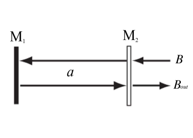
Figure 2: Open optical cavity. The cavity consists of two mirrors: $\mathrm{M_{1}}$ denotes a fully reflecting mirror and $\mathrm{M_{2}}$ denotes a partially transmitting mirror.

The cavity alone is modeled by a single quantum harmonic oscillator with Hamiltonian $H_{\rm cav}=\omega_{cav}a^{*}a$ with the resonance frequency $\omega_{cav}$ and the cavity annihilation operator $a$ is as defined before. However, the optical cavity in the figure will interact with an external EM field through the mirror $\mathrm{M}_{2}$, therefore it is an open quantum system. At this mirror there can be an exchange of photon between the cavity and the external field. It is convenient to work with the integrated version of the white noise field $B(t)=\int_{0}^{t}b(s)ds=(w_{q}(t)+iw_{p}(t))/2$, where $w_{q}(t)$ and $w_{p}(t)$ are self-adjoint non-commuting quantum Wiener processes. These processes can be realized as on symmetric Fock space over the space of square integrable complex functions [20, 15]. We remark that each of the processes $w_{q}(t)$ and $w_{p}(t)$ are individually isomorphic to a classical Wiener process but, since they do not commute, they cannot be realized on a common classical probability space.

As alluded to earlier, for the optical cavity, $L=\sqrt{\kappa}a$, where $a$ is the cavity annihilation operator. The joint dynamics of an open optical cavity coupled to the bosonic field $B(t)$ may be described by a unitary propagator $U(t)$ satisfying the quantum stochastic differential equation [20, 40],

$$dU(t)=\left(-(iH_{\rm cav}+\frac{\kappa}{2}a^{*}a)dt+\sqrt{\gamma}dB^{*}(t)a-\sqrt{\gamma}a^{*}dB(t)\right)U(t),$$

with initial condition $U(0)=1$. For each $t\geq 0$, the solution of this equation is unitary, $U(t)^{*}U(t)=U(t)U(t)^{*}=I$. The Heisenberg picture evolution of the cavity’s annihilation operator $a$ and creation operator $a^{*}$, are respectively, $a(t)=U(t)^{*}aU(t)$ and $a^{*}(t)=U(t)^{*}aU(t)$. They satisfy the linear quantum stochastic differential equation, [14, 15]:

$$\left[\begin{array}[]{c}da(t)\\ da^{*}(t)\\ \end{array}\right] = \left[\begin{array}[]{cc}-\frac{\kappa}{2}-i\omega_{cav}&0\\ 0&-\frac{\kappa}{2}+i\omega_{cav}\\ \end{array}\right]\left[\begin{array}[]{c}a(t)\\ a^{*}(t)\\ \end{array}\right]dt-\sqrt{\kappa}\left[\begin{array}[]{c}dB(t)\\ dB^{*}(t)\\ \end{array}\right].$$ (18)

After interacting with the cavity the field $B(t)$ also undergoes a transformation in the Heisenberg picture, yielding the output field $B_{\rm out}(t)=U(t)^{*}B(t)U(t)$. This is the field reflected from the cavity that contains any photons that have escaped from the cavity through the mirror $\mathrm{M}_{2}$, see Fig. 2. The output field $B_{\rm out}(t)$ satisfies the output equation:

$$dB_{out}(t) = \sqrt{\kappa}a(t)dt+dB(t).$$ (19)

2) Degenerate Parametric Amplifier: Now we briefly describe a degenerate parametric amplifier (DPA) as shown in Figure 3. It is an open oscillator with a classical pump that can produce squeezed output field (a field with reduced fluctuations along one of its quadratures and increased fluctuations on the conjugate quadrature). The pump field provides quanta and interacts with the cavity mode in a type of crystal called a $\chi^{(2)}$ crystal. In this crystal one photon from the pump field is annihilated to produce two photons of the cavity mode. The amplifier’s Hamiltonian can be written as

$$H_{SQ}=\omega_{cav}a^{*}a+\frac{i}{2}(\epsilon e^{-i\omega_{p}t}a^{*2}-\epsilon^{*}e^{i\omega_{p}t}a^{2}),$$

where $\omega_{p}$ is the frequency of the pump beam and $\epsilon$ a measure of the effective pump amplitude.

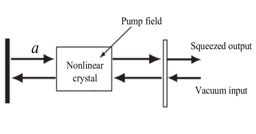
Figure 3: Degenerate parametric amplifier coupled to an bosonic field.

Following the same procedure as for the optical cavity, the Heisenberg picture dynamics of a degenerate parametric amplifier coupled to a bosonic field $B(t)$ is now given by (see [14, Chapter 10])

$$\left[\begin{array}[]{c}da(t)\\ da^{*}(t)\\ \end{array}\right] = \left[\begin{array}[]{cc}-\frac{\kappa}{2}-i\omega_{cav}&\epsilon e^{-i\omega_{p}t}\\ \epsilon^{*}e^{i\omega_{p}t}&-\frac{\kappa}{2}+i\omega_{cav}\\ \end{array}\right]\left[\begin{array}[]{c}a(t)\\ a^{*}(t)\\ \end{array}\right]dt-\sqrt{\kappa}\left[\begin{array}[]{c}dB(t)\\ dB^{*}(t)\\ \end{array}\right],$$

$$dB_{out}(t) = \sqrt{\kappa}a(t)dt+dB(t).$$

If we now switch to a rotating frame at half of the pump beam frequency $\omega_{p}/2$, we can remove the time-dependence in the system matrices to transform the system into a time-invariant one. This entails making the substitution $a(t)\rightarrow a(t)e^{-i\omega_{p}t/2}$, $a^{*}(t)\rightarrow a^{*}(t)e^{i\omega_{p}t/2}$, $B(t)\rightarrow B(t)e^{-i\omega_{p}t/2}$, $B^{*}(t)\rightarrow B^{*}(t)e^{i\omega_{p}t/2}$, and $B_{\rm out}(t)\rightarrow B_{\rm out}(t)e^{-i\omega_{p}t/2}$. These substitutions yield the time-invariant equation,

$$\left[\begin{array}[]{c}da(t)\\ da^{*}(t)\\ \end{array}\right] = \left[\begin{array}[]{cc}-\frac{\kappa}{2}-i(\omega_{cav}-\omega_{p}/2)&\epsilon\\ \epsilon^{*}&-\frac{\kappa}{2}+i(\omega_{cav}-\omega_{p}/2)\\ \end{array}\right]\left[\begin{array}[]{c}a(t)\\ a^{*}(t)\\ \end{array}\right]dt-\sqrt{\kappa}\left[\begin{array}[]{c}dB(t)\\ dB^{*}(t)\\ \end{array}\right],$$ (29)

$$dB_{out}(t) = \sqrt{\kappa}a(t)dt+dB(t).$$ (30)

The output field of a degenerate parametric amplifier as shown in Fig. 3 will be a squeezed field.

II-E3 More general model of open quantum stochastic systems

It can be seen from from (18)-(19) and (30), that the system coefficients are complex. However, for solving the control engineering problems, it is sometimes more convenient to work with systems with real-valued coefficients. Using the relations $x_{q_{1}}=Q(t)=a(t)+a^{*}(t)$, $x_{q_{2}}=P(t)=-i\left(a(t)-a^{*}(t)\right)$, $w_{1}^{\prime}(t)=B(t)+B^{*}(t)$, $w_{2}^{\prime}(t)=-i\left(B(t)-B^{*}(t)\right)$, $y_{q_{1}}=B_{out}(t)+B_{out}^{*}(t)$ and $y_{q_{2}}=-i\left(B_{out}(t)-B_{out}^{*}(t)\right)$, we can rewrite (18) and (19) in the quadrature representation (all system coefficients are real) as follows

$$dx_{q}(t) = \left[\begin{array}[]{cc}-\frac{\kappa}{2}&\omega_{cav}\\ -\omega_{cav}&-\frac{\kappa}{2}\\ \end{array}\right]x_{q}(t)dt-\sqrt{\kappa}dw^{\prime}(t),$$ (33)

$$dy_{q}(t) = \sqrt{\kappa}x_{q}(t)dt+dw^{\prime}(t),~{}~{}~{}t\geq 0,$$ (34)

where $x_{q}(t)=\left[\begin{array}[]{c}x_{q_{1}}\\ x_{q_{2}}\\ \end{array}\right]$, $y_{q}(t)=\left[\begin{array}[]{c}y_{q_{1}}\\ y_{q_{2}}\\ \end{array}\right]$ and $w^{\prime}(t)=\left[\begin{array}[]{c}w_{1}^{\prime}\\ w_{2}^{\prime}\\ \end{array}\right]$.

Similarly, (30) can be rewritten as

$$dx_{q}(t) = \left[\begin{array}[]{cc}-\frac{\kappa}{2}+\Re\{\epsilon\}&\quad\omega_{cav}-\omega_{p}/2+\Im\{\epsilon\}\\ -\omega_{cav}+\omega_{p}/2+\Im\{\epsilon\}&\quad-\frac{\kappa}{2}-\Re\{\epsilon\}\\ \end{array}\right]x_{q}(t)dt-\sqrt{\kappa}dw^{\prime}(t),$$ (37)

$$dy_{q}(t) = \sqrt{\kappa}x_{q}(t)dt+dw^{\prime}(t),~{}~{}~{}t\geq 0.$$ (38)

The optical cavity and degenerate parametric amplifier that we have briefly illustrated above are two important examples of linear quantum stochastic systems. We are now in the position to present a more general model for an open linear stochastic quantum system denoted by $G_{2}$ in the quadrature form given by

$$dx_{q}(t) = A_{qq}x_{q}(t)dt+B_{q}dw^{\prime}(t)+Eu(t)dt,$$ (39)

$$dy_{q}(t) = C_{qq}x_{q}(t)dt+D_{q}dw^{\prime}(t),$$ (40)

$$dy_{q}^{\prime}(t) = C^{\prime}_{qq}x_{q}(t)dt+D^{\prime}_{q}dw^{\prime}(t),~{}~{}~{}t\geq 0,$$ (41)

where $x_{q}(t)$ denotes $n_{q}$ pairs of amplitude and phase quadrature operators defined on a Hilbert space $\mathcal{H}$, $w^{\prime}(t)$ is a vector of $2m$ quantum stochastic processes that can be represented as self-adjont operators defined on a Fock space $F$, while $y_{q}(t)$ is a vector of $2n_{y_{q}}$ quantum outputs and $y_{q}^{\prime}(t)$ is a vector of $2n_{y_{q}^{\prime}}$ quantum outputs, such that $n_{y_{q}}+n_{y_{q}^{\prime}}\leq m$.

By the laws of quantum mechanics, the quantum system $G_{2}$ is required to possess the following properties; see [32, Section 2.5], [16] for a more detailed discussion.

(a)

The system variables preserve commutation relations, [23]:

$$[x_{q}(t),~{}x_{q}(t)^{T}]=[x_{q}(0),~{}x_{q}(0)^{T}]=2i\Theta_{n_{q}},~{}~{}t\geq 0,$$ (42)

where $\Theta_{n_{q}}$ is a skew-symmetric real matrix. Moreover, the matrix $\Theta_{n_{q}}$ is said to be canonical if it has the form $\Theta_{n_{q}}=\mathrm{diag}_{n_{q}}(J)$.

(b)

The system variables and the output satisfy the non-demolition condition [8], [9]:

$$\left[x_{q}(t),~{}\left[\begin{array}[]{c}y_{q}(r)\\ y_{q}^{\prime}(r)\\ \end{array}\right]^{T}\right]=0,~{}~{}~{}t\geq r\geq 0.$$ (43)

In other words, the current system variables are compatible with past outputs.

(c)

Define skew-symmetric real matrices $\Theta_{w}$ and $\Theta_{qq^{\prime}}$ by means of

$$\left[dw^{\prime}(t),~{}dw^{\prime}(t)^{T}\right] = 2i\Theta_{w},$$ (44)

$$\left[\left[\begin{array}[]{c}dy_{q}(t)\\ dy_{q}^{\prime}(t)\\ \end{array}\right],\left[\begin{array}[]{c}dy_{q}(t)\\ dy_{q}^{\prime}(t)\\ \end{array}\right]^{T}\right] = 2i\Theta_{qq^{\prime}},~{}~{}t\geq 0.$$ (49)

Then

$$\Theta_{qq^{\prime}}=\left[\begin{array}[]{c}D_{q}\\ D^{\prime}_{q}\\ \end{array}\right]\Theta_{w}\left[\begin{array}[]{c}D_{q}\\ D^{\prime}_{q}\\ \end{array}\right]^{T}.$$ (50)

This simply means that the quantum noise component at the output corresponds to a boson field, just like the input.

It turns out that the when

$$\left[\begin{array}[]{c}D_{q}\\ D^{\prime}_{q}\\ \end{array}\right]=[I_{2(n_{y_{q}}+n_{y_{q}^{\prime}})}\quad 0_{2(m-n_{y_{q}}-n_{y_{q}^{\prime}})}],$$ (51)

the above properties are guaranteed when the real constant matrices $A_{qq}$, $B_{q}$, $C_{qq}$, $D_{q}$, $C^{\prime}_{qq}$, and $D^{\prime}_{q}$ satisfy the so-called physical realizability conditions, [23, Theorem 3.4]:

$$B_{q}\Theta_{w}\left[\begin{array}[]{c}D_{q}\\ D^{\prime}_{q}\end{array}\right]^{T}=-\Theta_{n_{q}}[\begin{array}[]{cc}C_{qq}&C^{\prime}_{qq}\end{array}]^{T}$$ (55)

$$A_{qq}\Theta_{n_{q}}+\Theta_{n_{q}}A_{qq}^{T}+B_{q}\Theta_{w}B_{q}^{T}=0.$$ (56)

We remark that (51) is not the most general form possible for $[D_{q}^{T},(D^{\prime}_{q})^{T}]^{T}$. The general setting only requires that (50) holds without imposing any further conditions on the structure or form of $[D_{q}^{T},(D^{\prime}_{q})^{T}]^{T}$. Moreover, in the general setting the requirements for properties (a) and (b) are again given by (55) and (56), respectively [32, Theorems 2.1 and 2.2].

Remark 1

In fact, as shown in the proof of [23, Theorem 3.4], Eq. (42) is equivalent to Eq. (56). Moreover, noticing

$$\left[\left[\begin{array}[]{c}dy_{q}(t)\\ dy_{q}^{\prime}(t)\\ \end{array}\right],\left[\begin{array}[]{c}dy_{q}(t)\\ dy_{q}^{\prime}(t)\\ \end{array}\right]^{T}\right]=[dw^{\prime}(t),~{}dw^{\prime}(t)^{T}],$$

Eq. (51) leads to Eq. (50). Finally, for the special form of $D_{q}$ and $D_{q}^{\prime}$ as in Eq. (51), Eq. (43) is equivalent to Eq. (55).

Finally, since the system $G_{2}$ is a quantum linear system, it has an effective Hamiltonian of the form $H_{q}=\frac{1}{2}x_{q}^{T}R_{q}x_{q}+x_{q}^{T}K_{q}u(t)$, where $R_{q}=R_{q}^{T}\in\mathbb{R}^{2n_{q}\times 2n_{q}}$, and $K_{q}=-\Theta_{n_{q}}E\in\mathbb{R}^{2n_{q}\times 2m}$. The first term of $H_{q}$, namely $\frac{1}{2}x_{q}^{T}R_{q}x_{q}$, is the isolated Hamiltonian (also called free Hamiltonian) of the system $G_{2}$, while its second term $x_{q}^{T}K_{q}u(t)$, often called a control Hamiltonian, is induced by the coupling to the external environment through the classical signal $u(t)$ which is a vector of real locally square integrable functions. Some discussions on effective Hamiltonians for the linear case can be found in, e.g., [41, Chapter 6] (in particular Eq. (6.219) in [41]), and discussions on more general nonlinear case can be found in, e.g., [24, Eq. (2) and Sec. 5] and [38, Sec. 1-C]. More details on the implementation of $x_{q}^{T}K_{q}u$ using classical devices can be found in, e.g., [46], [17].

II-F Mixed quantum-classical linear stochastic systems with quantum inputs and quantum outputs

Equations (39)-(41) look superficially like the classical state space equations familiar to control engineers, but in fact are fundamentally different because they are equations for a collection of quantum degrees of freedom (noncommutative variables), not a collection of classical degrees of freedom (commutative variables). Even so, the classical system described by (5)-(7) and the quantum system given by (39)-(41) may be interconnected as a mixed quantum-classical system via appropriate interfaces (homodyne detectors and modulators). As introduced in Subsection II-C, any classical probability model ($\Omega,F,\nu$) can be viewed as a commutative quantum probability model ($\mathcal{A},\rho$), which means that classical components can be treated within the formalisms of quantum mechanics by embedding them as commutative subsystem in a quantum system. The problem of putting quantum and classical degrees of freedom within the same formalism has also been discussed in [33, 37, 23, 15, 31, 34] and the references therein. In particular, in the physics literature the formalism is known as the Koopman-von Neumann formulation (of classical mechanics) and the embedding of a classical dynamical system in a quantum one is referred to as a “quantum mechanics-free subsystem” [34]. In this paper, we aim to develop a mathematical representation for a class of mixed quantum-classical linear stochastic systems.

We briefly review some results about mixed quantum-classical linear stochastic systems with quantum inputs and quantum outputs studied in [23] and [31]. Let $x$ have both quantum and classical degrees of freedom, such that $x=[x_{q}^{T}\quad x_{c}^{T}]^{T}$. To be interpreted a classical variable, we require that the entries of ${x}_{c}(t)$ commute with one another and with entries of the vector of quantum observables $x_{q}(t)$. Thus, the commutation relation for $x(t)$ satisfies

$$[x(t),~{}x(t)^{T}]=2i\Theta_{n},$$

where $\Theta_{n}=\mathrm{diag}(\Theta_{n_{q}},0_{n_{c}\times n_{c}})$. In particular, if $\Theta_{n_{q}}=\mathrm{diag}_{n_{q}}(J)$, then $\Theta_{n}$ is said to be degenerate canonical, [23]. Actually, we require more, that $x_{c}(t)$ is isomorphic to a classical stochastic process. That is, $[x_{c}(t),x_{c}(s)]^{T}=0$ for all $s\geq 0$ not necessarily equal to $t$. This does in fact hold, and we will say more about this immediately after Theorem 1. Following [23], we thus consider a linear mixed quantum-classical system of the form

$$dx(t) = Ax(t)dt+Bdw(t),$$ (57)

$$dy_{q}(t) = C_{q}x(t)dt+D_{q}dw(t),$$ (58)

where $w(t)$ and $y_{q}(t)$ are quantum input and output fields, respectively, and $A\in\mathbb{R}^{n\times n}$, $B\in\mathbb{R}^{n\times 2m}$, $C_{q}\in\mathbb{R}^{2n_{y_{q}}\times n}$ and $D_{q}\in\mathbb{R}^{2n_{y_{q}}\times 2m}$, $n=2n_{q}+n_{c}$. As discussed in Subsection II-C, if we are given a component of a vector of classical system variables $x_{c}$ denoted by $x_{c_{k}}$, we may consider $x_{c_{k}}$ as one of the quadratures of a quantum harmonic oscillator, say the amplitude quadrature $q_{k}$. Then we may define an augmentation of $x_{c_{k}}(t)$, say $\tilde{x}_{k}(t)=\left[\begin{array}[]{c}q_{k}(t)\\ p_{k}(t)\\ \end{array}\right]$. Therefore, $x(t)$ can be embedded in a larger vector $\tilde{x}(t)=[x(t)^{T}\quad\eta(t)^{T}]^{T}$, where any element of $\eta(t)=[p_{1}(t)~{}p_{2}(t)~{}\cdots~{}p_{n_{c}}(t)]^{T}$ commutes with any component of $x_{q}(t)$, and are conjugate to the components of $x_{c}(t)$, satisfying $[x_{c_{j}}(t),\eta_{k}(t)]=2i\delta_{jk}$, where $\delta_{jk}$ is the Kronecker delta function. As a result, the commutation relation for $\tilde{x}(t)$ is $[\tilde{x}(t),~{}\tilde{x}(t)^{T}]=2i\tilde{\Theta}$, where

$$\tilde{\Theta}\!=\!\!\left[\!\begin{array}[]{cc}\Theta_{n}&\left[\begin{array}[]{c}0\\ I_{n_{c}}\\ \end{array}\right]\\ \left[\begin{array}[]{cc}0&-I_{n_{c}}\\ \end{array}\right]&0\\ \end{array}\!\right]$$

is an invertible matrix satisfying $\tilde{\Theta}\tilde{\Theta}=-I$ and $\tilde{\Theta}=-\tilde{\Theta}^{T}$. Moreover, as shown in [23], there is an augmentation of the system (57)-(58) in terms of $\tilde{x}$, which can be written as

$$d\tilde{x}(t) = \tilde{A}\tilde{x}(t)dt+\tilde{B}dw(t),$$ (59)

$$dy_{q}(t) = \tilde{C}\tilde{x}(t)dt+D_{q}dw(t),$$ (60)

where $\tilde{A}\!\!=\!\!\left[\begin{array}[]{cc}A&0\\ A^{\prime}&A^{\prime\prime}\\ \end{array}\right]$, $\tilde{B}\!=\!\!\left[\begin{array}[]{c}B\\ B^{\prime}\\ \end{array}\right]$, and $\tilde{C}\!=\!\!\left[\begin{array}[]{cc}C_{q}\quad 0\\ \end{array}\right]$.

We first have the following definition when $D_{q}$ takes on a particular form.

Definition 1

[[23]] Let $D_{q}=I_{2m}$ or $D_{q}=[I_{2n_{y_{q}}}\quad 0_{2(m-n_{y_{q}})}]$. The mixed quantum-classical system (57)-(58) with quantum inputs and quantum outputs is physically realizable if there exists an augmentation of the form (59) and (60) that is a physically realizable fully quantum system. That is, if there exist matrices $A^{\prime}$, $A^{\prime\prime}$, $B^{\prime}$ such that (55)-(56) hold with matrices $A_{qq}$, $B_{q}$, $\left[\begin{array}[]{c}C_{qq}\\ C^{\prime}_{qq}\\ \end{array}\right]$ and $\left[\begin{array}[]{c}D_{q}\\ D^{\prime}_{q}\\ \end{array}\right]$ replaced by corresponding matrices $\tilde{A}$, $\tilde{B}$, $\tilde{C}$, $D_{q}$, respectively.

The following result gives the physical realizability conditions for the mixed quantum-classical system (57)-(58) that follow from those for the fully quantum system (59)-(60). Note that the conditions below do not depend on $A^{\prime}$, $A^{\prime\prime}$, $B^{\prime}$. That is, the conditions are intrinsic on the system (57)-(58). If these conditions are fulfilled then there exist suitable choices of $A^{\prime}$, $A^{\prime\prime}$, $B^{\prime}$ to construct a physically realizable augmentation.

Theorem 1

[[23]] Let $D_{q}=I_{2m}$ or $D_{q}=[I_{2n_{y_{q}}}\quad 0_{2(m-n_{y_{q}})}]$. The mixed quantum-classical system (57)-(58) with quantum inputs and quantum outputs is physically realizable if and only if

$$A\Theta_{n}+\Theta_{n}A^{T}+B{\rm diag}_{m}(J)B^{T}=0,$$

$$\Theta_{n}C^{T}=-B{\rm diag}_{m}(J)D_{q}^{T}.$$

From the above theorem, it will be guaranteed that $[x(t),x(t)^{T}]=2i\Theta_{n}$ for all $t\geq 0$. However, as alluded to earlier, for $x_{c}(t)$ to be interpretable as a classical stochastic process, we require that $[x_{c}(t),x_{c}(s)^{T}]=0$ for all $s\geq 0$ not necessarily equal to $t$. In a more general setting to be given in Definition 4, we make this explicit by imposing the requirement that the entries of $x_{c}(t)$ commute will every entry of $x_{c}(s)$ for any time $s\geq 0$ not necessarily equal to $t$. That this is indeed the case will be seen in the proof of Theorem 3 where it emerges as an easy consequence of the equal time commutation relations $[x_{c}(t),x(t)^{T}]=0$. In other words, the equal time commutation relations that forms a basis for the physical realizability of the augmentation (59) and (60) is enough to characterize the mixed quantum-classical system given by (57)-(58). Yet another way to view this is that the definition of physical realizability in Definition 1 given through an augmentation of (57)-(58) is perfectly consistent with $x_{c}(t)$ being isomorphic to a classical stochastic process, despite the fact that this requirement is not explicitly stated in the definition.

Remark 2

We have the following observations for the abstractly defined mixed quantum-classical linear stochastic system (57)-(58) with quantum inputs and outputs, as studied in [23]:

(a)

The inputs and outputs are all purely quantum;

(b)

The matrix $D_{q}$ is in the form of $D_{q}=I_{2m}$ (or $D_{q}=[I_{2n_{y_{q}}}\quad 0_{2(m-n_{y_{q}})}]$ if $n_{y_{q}}<m$).

(c)

It is not immediately apparent how quantum and the classical components are interconnected and what are the interfaces that are required make the interconnection.

In the sections that will follow, we will relax the requirements (a) and (b) and also address (c) in a more general setting.

III Canonical representation of mixed linear stochastic systems

In this section, we give two forms for mixed quantum-classical linear stochastic systems described by LSDEs, one being a general form in which the mixed system is often obtained in real experiments and the other being a standard form in which the mixed system can be easily decomposed for analysis and synthesis. We also derive relations between the two forms. Notice that in this paper we allow the general form to include classical inputs and outputs as well as scattering processes, which are more general than the mixed quantum-classical linear stochastic systems of the form (57)-(58) with quantum inputs and outputs, as discussed in Subsection II-F; cf. Remark 2.

III-A A standard form for mixed linear stochastic systems with quantum inputs and mixed outputs

Consider the following mixed linear stochastic system with quantum inputs and mixed outputs:

$$dx(t) = Ax(t)dt+Bdw(t),$$ (61)

$$dy(t) = Cx(t)dt+Ddw(t).\$$ (62)

As specified before, the system variables are $x=[x_{q}^{T}\quad x_{c}^{T}]^{T}$, the system outputs are $y=[y_{q}^{T}\quad y_{c}^{T}]^{T}$. Define a constant real matrix $F_{y}$ by

$$dy(t)dy(t)^{T}=F_{y}dt.$$ (63)

Also, define a real skew-symmetric matrix $\Theta_{y_{q}}$ in terms of

$$[dy_{q}(t),~{}dy_{q}(t)^{T}]=2i\Theta_{y_{q}}.$$ (64)

Clearly, the mixed output $y_{q}(t)$ is a vector of dimension $n_{y}=2n_{y_{q}}+n_{y_{c}}$. For later use, the system input $w(t)$ is partitioned to be $w(t)=[w_{1}(t)^{T}\quad w_{2}(t)^{T}]^{T}$ where $w_{1}(t)$ is of dimension $2n_{w_{1}}$ and $w_{2}(t)$ is of dimension $2n_{w_{2}}$. However, instead of being of the form $I$ or $[\begin{array}[]{cc}I&0\end{array}]$ as in Eq. (51), or equivalently $D_{q}$ specified in Theorem 1, in general, the matrix $D$ is associated with gauge processes representing the photon exchange among the external fields represented here by $w(t)$.

Remark 3

It will be shown later in Remark 7 that

$$[dw(t),~{}dw(t)^{T}]=2i\Theta_{w},$$ (65)

where the skew-symmetric matrix $\Theta_{w}$ is given in Eq. (44).

The transfer function for system (61)-(62) is

$$\Xi_{S}(s)=\left[\begin{tabular}[]{l|ll}$A$&$B$\\ \hline\cr\vspace{-2em}\\ $C$&$D$\\ \end{tabular}\right](s)=C\left(sI_{n}-A\right)^{-1}B+D.$$

Definition 2

The mixed quantum-classical linear stochastic system (61)-(62) is said to be standard if the following holds:

1. $\Theta_{n}=\mathrm{diag}(\Theta_{n_{q}},0_{n_{c}\times n_{c}})$ with $\Theta_{n_{q}}=\mathrm{diag}_{n_{q}}(J)$.

2. $\Theta_{w}=\mathrm{diag}_{m}(J)$.

3. The matrix $F_{y}$ defined in Eq. (63) satisfies $F_{y}=I_{n_{y}}+i\,\mathrm{diag}(\Theta_{y_{q}},0_{n_{{y_{c}}}\times n_{{y_{c}}}})$, where $\Theta_{y_{q}}=\mathrm{diag}_{n_{y_{q}}}(J)$.

Now let the matrices $A$, $B$, $C$, $D$ be partitioned compatibly with partitioning of $x(t)$ into $x_{q}(t)$ and $x_{c}(t)$ as

$$A=\left[\begin{array}[]{cc}A_{qq}&A_{qc}\\ A_{cq}&A_{cc}\\ \end{array}\right],\quad B=\left[\begin{array}[]{c}B_{q}\\ B_{c}\\ \end{array}\right],\quad C\!=\left[\begin{array}[]{c}C_{q}\\ C_{c}\\ \end{array}\right]\!=\!\left[\begin{array}[]{cc}C_{qq}&C_{qc}\\ C_{cq}&C_{cc}\\ \end{array}\right],\quad D=\left[\begin{array}[]{c}D_{q}\\ D_{c}\\ \end{array}\right].$$ (67)

Then, the system (61)-(62) can be rewritten as follows:

$$dx_{q}(t) = [\begin{array}[]{cc}A_{qq}\quad A_{qc}\\ \end{array}]x(t)dt+B_{q}dw(t),$$ (69)

$$dx_{c}(t) = [\begin{array}[]{cc}A_{cq}\quad A_{cc}\\ \end{array}]x(t)dt+B_{c}dw(t),$$ (71)

$$dy_{q}(t) = [\begin{array}[]{cc}C_{qq}\quad C_{qc}\\ \end{array}]x(t)dt+D_{q}dw(t),$$ (73)

$$dy_{c}(t) = [\begin{array}[]{cc}C_{cq}\quad C_{cc}\\ \end{array}]x(t)dt+D_{c}dw(t).$$ (75)

Remark 4

The features presented in Definition 2 allow us to consider classical variables $x_{c}(t)$, characterized by zero commutation relations, as well as classical noise processes $y_{c}(t)$, corresponding to the absence of the imaginary part in the Ito products, [23], [31]. The first item of Definition 2 indicates that $x(t)$ has both quantum and classical degrees of freedom, where $\Theta_{n_{q}}$ corresponds to the quantum degrees of freedom $x_{q}(t)$, while $0_{n_{c}\times n_{c}}$ corresponds to the classical degrees of freedom $x_{c}(t)$. The second item of Definition 2 shows that input signals of the system (61)-(62) are fully quantum. Finally, let

$$\Theta_{y}=\frac{[dy(t),~{}dy(t)^{T}]}{2i}=\frac{F_{y}-(F_{y})^{T}}{2i}.$$

Clearly,

$$\Theta_{y}=\mathrm{diag}(\Theta_{y_{q}},0_{n_{y_{c}}}).$$

Therefore, the third item of Definition 2 implies that $\Theta_{y_{q}}$ corresponds to quantum outputs $y_{q}(t)$ while the matrix $0_{n_{y_{c}}}$ corresponds to classical outputs $y_{c}(t)$. Finally, in analogy to Eq. (50), we have

$$\Theta_{y}=D\Theta_{w}D^{T}.$$ (76)

Remark 5

The difference between the mixed linear systems (57)-(58) and (61)-(62) is that the latter explicitly exhibits classical output signals, and the matrix $D$ has a more general form satisfying condition (76), which is equivalent to the following equations:

$$D_{q}\Theta_{w}D^{T}_{q} = \Theta_{y_{q}},$$ (77)

$$D_{q}\Theta_{w}D^{T}_{c} = 0,$$ (78)

$$D_{c}\Theta_{w}D^{T}_{c} = 0.$$ (79)

III-B A general form for mixed linear stochastic systems with mixed inputs and mixed outputs

In Definition 2, the quantum-classical nature of the standard form is captured in the matrices $\Theta_{n}$, $\Theta_{w}$, $F_{y}$ specifying the commutation relations of the system and signal. In general, we may take the commutation matrix to be an arbitrary real skew-symmetric matrix, while the Ito matrix $F$ is a free non-negative Hermitian matrix. To this end, consider a general form for linear mixed quantum-classical stochastic systems given by

$$d\mathbf{x}(t) = \mathbf{A}\mathbf{x}(t)dt+\mathbf{B}dv(t),$$ (80)

$$d\mathbf{y}(t) = \mathbf{C}\mathbf{x}(t)dt+\mathbf{D}dv(t),$$ (81)

where $\mathbf{A}\in\mathbb{R}^{n\times n}$, $\mathbf{B}\in\mathbb{R}^{n\times n_{v}}$, $\mathbf{C}\in\mathbb{R}^{n_{\mathbf{y}}\times n}$ and $\mathbf{D}\in\mathbb{R}^{n_{\mathbf{y}}\times n_{v}}$; $\mathbf{x}(t)$ includes quantum and classical system variables satisfying the commutation relation, such that $[\mathbf{x}(t),~{}~{}(\mathbf{x}(t))^{T}]=2i\hat{\Theta}_{n}$ with a skew-symmetric matrix $\hat{\Theta}_{n}$; the vector $v(t)$ represents the input signals, which contains quantum and classical noises; $\mathbf{y}(t)$ represents mixed quantum-classical outputs. $F_{v}$ and $F_{\mathbf{y}}$ are nonnegative definite Hermitian matrices satisfying $dv(t)dv(t)^{T}=F_{v}dt$ and $d\mathbf{y}(t)d\mathbf{y}(t)^{T}=F_{\mathbf{y}}dt$. Define

$$\Theta_{\bf y}=\frac{F_{\bf y}-(F_{\bf y})^{T}}{2i}.$$

The transfer function $\Xi_{G}(s)$ for a system of the form (80)-(81) is given by

$$\Xi_{G}(s)=\left[\begin{tabular}[]{l|ll}$\mathbf{A}$&$\mathbf{B}$\\ \hline\cr\vspace{-2em}\\ $\mathbf{C}$&$\mathbf{D}$\\ \end{tabular}\right](s)=\mathbf{C}\left(sI_{n}-\mathbf{A}\right)^{-1}\mathbf{B}+\mathbf{D}.$$

III-C Relations between the General and Standard Forms

The standard form (61)-(62) and the general form (80)-(81) can be related by the following lemmas and theorem:

Lemma 1

Given an arbitrary $n\times n$ real skew-symmetric matrix $\hat{\Theta}_{n}$ ($n\geq 2$), there exists a real nonsingular matrix $P_{n}$ and a block diagonal matrix $\Theta_{n}=\mathrm{diag}(\Theta_{n_{q}},0_{n_{c}\times n_{c}})$ such that

$$\Theta_{n}=P_{n}\hat{\Theta}_{n}P_{n}^{T}.$$ (83)

A similar proof of Lemma 1 can be found in [21, Theorem 2.5.8] and hence the proof is omitted here.

Lemma 2

Given an arbitrary $m\times m$ nonnegative definite Hermitian matrix $F_{v}$, there exists a $2m\times 2m$ matrix $F_{w}$=$I_{2m}$+$i\ \mathrm{diag}_{m}(J)$ and a $m\times 2m$ real matrix $W$ such that

$$F_{v}=WF_{w}W^{T}.$$ (84)

Proof: Hermitian matrices $F_{v}$ and $F_{w}$ can be diagonalized by unitary matrices $U_{v}$ and $U_{w}$, respectively, such that

$$F_{v} = U_{v}\Lambda_{v}U_{v}^{\dagger},$$ (85)

$$F_{w} = U_{w}\Lambda_{w}U_{w}^{\dagger},$$ (86)

where $\Lambda_{v}$=diag$(\lambda_{1},\lambda_{2},\cdots\lambda_{m})$, ($\lambda_{j}\geq 0$ is an eigenvector of $F_{v}$), $\Lambda_{w}$=diag${}_{m}\left(\left[\begin{array}[]{cc}0,&0\\ 0,&2\\ \end{array}\right]\right)$, $U_{w}$=diag${}_{m}\left(\frac{\sqrt{2}}{2}\left[\begin{array}[]{cc}i,&i\\ -1,&1\\ \end{array}\right]\right)$. Since $\Lambda_{v}$ and $\Lambda_{w}$ are two real diagonal matrices, there exists a $m\times 2m$ complex matrix $Q=[q_{1},q_{2},\cdots,q_{2m}]$ such that

$$\Lambda_{v}=Q\Lambda_{w}Q^{\dagger}.$$ (87)

In order to let (87) hold, for simplicity we choose $q_{2}=\left[\begin{array}[]{cccc}\sqrt{\frac{\lambda_{1}}{2}}&0&\cdots&0\\ \end{array}\right]^{T}$ , $q_{4}=\left[\begin{array}[]{ccccc}0&\sqrt{\frac{\lambda_{2}}{2}}&0&\cdots&0\\ \end{array}\right]^{T}$, $\cdots$, $q_{2m}=\left[\begin{array}[]{cccc}0&\cdots&0&\sqrt{\frac{\lambda_{m}}{2}}\end{array}\right]^{T}$, and $q_{1},q_{3},\cdots,q_{2m-1}$ now are arbitrary column vectors of length $m$ and to be determined later. Combining (85), (86) and (87) gives

$$F_{v}=U_{v}QU_{w}^{\dagger}F_{w}(UQU_{w}^{\dagger})^{\dagger}.$$ (88)

Let $W$ be defined as $W=U_{v}QU_{w}^{\dagger}$. Then we have

$$U_{v}Q=[U_{v}q_{1},U_{v}q_{2},\cdots,U_{v}q_{2m}].$$ (89)

Next, we will show that $Q$ can be chosen to let $W$ be real. Observing the structure of $U_{w}$, such that

$$U_{w}=\mathrm{diag}_{m}\left(\frac{\sqrt{2}}{2}\left[\begin{array}[]{cc}i,&i\\ -1,&1\\ \end{array}\right]\right),$$

we require that $q_{1},q_{3},\cdots,q_{2m-1}$ be chosen as

$$q_{1}=-U_{v}^{\dagger}U_{v}^{\#}q_{2},\quad q_{3}=-U_{v}^{\dagger}U_{v}^{\#}q_{4},\quad\cdots,\quad q_{2m-1} = -U_{v}^{\dagger}U_{v}^{\#}q_{2m}.$$

The matrix $Q$ is hence constructed as

$$Q=\left[\begin{array}[]{ccccccc}-U_{v}^{\dagger}U_{v}^{\#}q_{2},&q_{2},&-U_{v}^{\dagger}U_{v}^{\#}q_{4},&q_{4},&\cdots&-U_{v}^{\dagger}U_{v}^{\#}q_{2m},&q_{2m}\\ \end{array}\right].$$

We can get the representation (84) with $W=U_{v}QU_{w}^{\dagger}$. $\blacksquare$

Let us look at an example applying Lemma 2.

$\mathbf{Example\ 1}$: Consider a nonnegative definite Hermitian matrix given by

$$F_{v}\!=\!\!\left[\!\!\!\begin{array}[]{ccc}8.9286&-0.2143+4.8107i&0.1429+7.2161i\\ -0.2143-4.8107i&8.3571+0.0000i&0.4286-2.4054i\\ 0.1429-7.2161i&0.4286+2.4054i&8.7143\\ \end{array}\!\!\!\right].$$

It is easily obtained that $F_{v}=U_{v}\Lambda_{v}U^{\dagger}$ with

$$U_{v}=\left[\!\!\begin{array}[]{ccc}0.6814&0.6814&0.2673\\ -0.1572-0.3922i&-0.1572+0.3922i&0.8018\\ 0.1048-0.5883i&0.1048+0.5883i&-0.5345\\ \end{array}\right]$$

and

$$\Lambda_{v}=\left[\begin{array}[]{ccc}18&0&0\\ 0&0&0\\ 0&0&8\\ \end{array}\right].$$

Now following the construction in the proof of Lemma 2, we want to find a real matrix $W$. Choosing $q_{2}=[3\quad 0\quad 0]^{T},q_{4}=[0\quad 0\quad 0]^{T}$ and $q_{6}=[0\quad 0\quad 2]^{T}$ we get $q_{1}=[0\quad-3\quad 0]^{T},q_{3}=[0\quad 0\quad 0]^{T}$ and $q_{5}=[0\quad 0\quad-2]^{T}$. So the matrix $Q=\left[\begin{array}[]{cccccc}0&3&0&0&0&0\\ -3&0&0&0&0&0\\ 0&0&0&0&-2&2\\ \end{array}\right]$. It follows from the above construction that $W=\left[\begin{array}[]{cccccc}0&2.8909&0&0&0&0.7559\\ -1.6641&-0.6671&0&0&0&2.2678\\ -2.4962&0.4447&0&0&0&-1.5119\\ \end{array}\right]$. It is easily checked that $F_{v}=WF_{w}W^{T}$ with $F_{w}$=$I_{6}$+$i\ \mathrm{diag}_{3}(J)$.

Theorem 2

Given a mixed quantum-classical stochastic system of the general form (80)-(81), there exists a corresponding standard form (61)-(62).

Proof: By Lemmas 1 and 2, there exist matrices $P_{n}$, $W$ and $P_{\mathbf{y}}$ such that the coordinate transformations

$$x=P_{n}{\bf x},\quad y=P_{\mathbf{y}}\mathbf{y},\quad w=W^{T}v$$

yields

$$\left.\begin{array}[]{ccc}\Theta_{n}=P_{n}\hat{\Theta}_{n}P_{n}^{T},\quad\Theta_{y}=P_{\mathbf{y}}\Theta_{\mathbf{y}}P_{\mathbf{y}}^{T},\quad\Theta_{v}=W\Theta_{w}W^{T},\\ \quad A=P_{n}\mathbf{A}P_{n}^{-1},\quad B=P_{n}\mathbf{B}W,\quad C=P_{\mathbf{y}}\mathbf{C}P_{n}^{-1},\quad D=P_{\mathbf{y}}\mathbf{D}W.\\ \end{array}\right\}$$ (93)

Substituting (93) into (80)-(81) gives (61)-(62). Now, we can verify the following relation between the standard $\Xi_{S}(s)$ and general $\Xi_{G}(s)$ transfer functions:

$$\Xi_{S}(s) = C\left(sI_{n}-A\right)^{-1}B+D$$

$$= P_{\mathbf{y}}\mathbf{C}P_{n}^{-1}\left(sP_{n}P_{n}^{-1}-P_{n}\mathbf{A}P_{n}^{-1}\right)^{-1}P_{n}\mathbf{B}W+P_{\mathbf{y}}\mathbf{D}W$$

$$= P_{\mathbf{y}}\left(\mathbf{C}\left(sI_{n}-\mathbf{A}\right)^{-1}\mathbf{B}+\mathbf{D}\right)W$$

$$= P_{\mathbf{y}}\Xi_{G}(s)W.\vspace{-1em}$$

Thus, the general form (80)-(81) can be linearly transformed into its corresponding standard form (61)-(62). $\blacksquare$

IV Physical realizability of mixed quantum-classical linear stochastic systems

In this section, we will introduce the definition of physical realizability of the standard form (61)-(62) and a theorem on necessary and sufficient conditions for its physical realizability. Analogous physical realizability definition and conditions for the general form (80)-(81) are also presented in this section.

IV-A Physical realizability for the standard form

The following concepts and lemmas will be used for introducing the definition of physical realizability of the system (61)-(62).

The Belavkin’s nondemolition principle requires an observable $X(t)$ at a time instant $t$ to be compatible with the past output process $Y(s)$ ($s\leq t$) [8], [9], that is:

$$[X(t),~{}Y(s)^{T}]=0,\ \forall\ t\geq s\geq 0.$$ (94)

Condition (94) is known as non-demolition condition.

Lemma 3

Non-demolition condition $[\tilde{x}(t),~{}y_{q}(s)^{T}]=0$, $\forall$ $t\geq s\geq 0$ for the augmented system (59)-(60) of the system (57)-(58) holds, if and only if

$$\tilde{B}\Theta_{w}D_{q}^{T}=-\tilde{\Theta}\tilde{C}^{T}.$$ (95)

Proof: First, we will argue that $[\tilde{x}(t),y_{q}(s)^{T}]=0$ is equivalent to $[\tilde{x}(t),y_{q}^{T}(t)]=0$, for all $t\geq s\geq 0$. Let $g_{s}(t)=[\tilde{x}(t),y_{q}(s)^{T}]$, for all $t\geq s\geq 0$, where $s$ is fixed. From $[\tilde{x}(t),y_{q}(t)^{T}]=0$ for all $t\geq s\geq 0$, we can infer that $g_{s}(s)=0$ and then have

$$dg_{s}(t) = d[\tilde{x}(t),y_{q}(s)^{T}]$$

$$= [d\tilde{x}(t),y_{q}(s)^{T}]$$

$$= \tilde{A}[\tilde{x}(t),y_{q}(s)^{T}]dt$$

$$= \tilde{A}g_{s}(t)dt.$$

Solving the above equation gives $g_{s}(t)=\mathrm{exp}\left(\tilde{A}(t-s)\right)g_{s}(s)=0$. Therefore, $[\tilde{x}(t),y_{q}(t)^{T}]=0$ implies $[\tilde{x}(t),y_{q}(s)^{T}]=0$, for all $t\geq s\geq 0$. Conversely, it is trivial to verify that $[\tilde{x}(t),y_{q}(s)^{T}]=0$ for all $t\geq s\geq 0$ implies $[\tilde{x}(t),y_{q}(t)^{T}]=0$ for all $t\geq 0$.

Thus, we just need to consider the case where $t=s$. Let $g(t)=[\tilde{x}(t),y_{q}(t)^{T}]$ with $g(0)=0$ and then we have

$$dg(t) = d[\tilde{x}(t),y_{q}(t)^{T}]$$

$$= [d\tilde{x}(t),y_{q}(t)^{T}]+[\tilde{x}(t),dy_{q}(t)^{T}]+[d\tilde{x}(t),dy_{q}(t)^{T}]$$

$$= \tilde{A}g(t)dt+2i(\tilde{\Theta}\tilde{C}^{T}+\tilde{B}\Theta_{w}D_{q}^{T})dt.$$

Solving the above equation gives

$$g(t)=\mathrm{exp}(\tilde{A}t)g(0)+2i\int^{t}_{0}\mathrm{exp}(\tilde{A}(t-\tau))\left(\tilde{\Theta}\tilde{C}^{T}+\tilde{B}\Theta_{w}D_{q}^{T}\right)d\tau.$$ (96)

It can be easily verified from (96) that $g(t)=0$ holds for all $t\geq 0$, if and only if $\tilde{\Theta}\tilde{C}^{T}+\tilde{B}\Theta_{w}D_{q}^{T}=0$, which is Eq. (95). $\blacksquare$

Lemma 4

Non-demolition condition $[x(t),y(s)^{T}]=0$, $\forall$ $t\geq s\geq 0$ for the system (61)-(62) holds, if and only if

$$B\Theta_{w}D^{T}=-\Theta_{n}C^{T}.$$ (97)

The proof of Lemma 4 is similar to that of Lemma 3 and is thus omitted.

For a better understanding of Definitions 3 and 4 to be given later, a discussion regarding the physical realizability of the standard form (61)-(62) will be given first. The system (61)-(62) can be divided into two parts: one is the system (57)-(58), or equivalently the system (69)-(73), with $D_{q}$ satisfying Eq. (77); the other is the output equation (75). Therefore, the system (61)-(62) is physically realizable if the two parts are both physically realizable. First, we consider physical realizability conditions of the system (57)-(58). From the structure of system matrices of the augmented system (59)-(60), it is clear that the dynamics of $x(t)$ of system (57)-(58) embedded in system (59)-(60) are not affected by the augmentation, and moreover, it will be shown in the proof of Theorem 3 below that matrices $A^{\prime},A^{\prime\prime},B^{\prime}$ in system (59)-(60) can be chosen to preserve commutation relations for augmented system variables $\tilde{x}$ . As given in Definition 1, the system (57)-(58) with $D_{q}$ satisfying (77) is physically realizable if its augmented system (59)-(60) is physically realizable, with explicit physical realizability conditions stated in Theorem 1. It is worthing noting that these physical realizability conditions are only suitable for an augmented system (59)-(60) with $D_{q}=I$ or $D_{q}=[\begin{array}[]{cc}I&0\end{array}]$ (no scattering processes involved). However, the matrix $D_{q}$ in the standard form system (59)-(60) is allowed to be more general, namely, the one satisfying Eq. (77). To deal with this, we need to extend the physical realizability condition of the system (59)-(60) by allowing a general matrix $D_{q}$ satisfying Eq. (77). We first transform the augmented system (59)-(60) into a familiar form without scattering processes. Suppose that non-demolition condition $[\tilde{x}(t),y_{q}(s)^{T}]=0$, $\forall$ $t\geq s\geq 0$ holds. So, we apply Eq. (95) in Lemma 3 to the quantum output $y_{q}$ in Eq. (60) to get $y_{q}=D_{q}\bar{y}_{q}$ with $\bar{y}_{q}$ defined as $d\bar{y}_{q}=\bar{C}\tilde{x}(t)dt+dw(t)$, where $\bar{C}=\Theta_{w}\tilde{B}^{T}\tilde{\Theta}$. Then, a reduced system for the augmented system (59)-(60) is defined as

$$d\tilde{x}(t) = \tilde{A}\tilde{x}(t)dt+\tilde{B}dw(t),$$ (98)

$$d\bar{y}_{q} = \bar{C}\tilde{x}(t)dt+dw(t).$$ (99)

It is straightforward to verify that the reduced system (98)-(99) is physically realizable in the sense of Definition 1 and satisfying the conditions of Theorem 1. The definition of physical realizability of an augmented system of the system (57)-(58) is as follows:

Definition 3

An augmentation (59)-(60) of the system (57)-(58) with a general matrix $D_{q}$ is said to be physically realizable if the following statements hold:

1. The reduced system (98)-(99) is physically realizable in the sense of Definition 1.

2. For the augmented system (59)-(60), non-demolition condition $[\tilde{x}(t),y_{q}(s)^{T}]=0,\ \forall\ t\geq s\geq 0$ holds.

3. $D_{q}$ is of the form $[\begin{array}[]{cc}I_{n_{y_{q}}}&0\end{array}]\tilde{V}$ with $\tilde{V}$ a symplectic matrix [16] or unitary symplectic [30] such that relation (77) holds.

Next we will consider physical realizability conditions of the system (75). Classical systems are always regarded as being physically realizable since they can be approximately built via digital and analog circuits. Thus, we just need to make sure that output equation (75) is classical. Now, we can present a formal definition of physical realizability of the system (61)-(62).

Definition 4

A system of the standard form (61)-(62) is said to be physically realizable if the following statements hold:

1. There exists an augmented system (59)-(60) of the system (57)-(58) with $D_{q}$ satisfying (77), which is physically realizable in the sense of Definition 3.

2. For the system (61)-(62), non-demolition condition $[x(t),~{}y(s)^{T}]=0,\ \forall\ t\geq s\geq 0$ holds.

3. The output (75) and system variables $x_{c}$ both represent classical stochastic processes in the sense of the following commutation relations $[x_{c}(t),~{}x^{T}_{c}(s)]=0$, $[x_{c}(t),~{}y^{T}_{c}(s)]=0$, and $[y_{c}(t),~{}y^{T}_{c}(s)]=0$ for all $t,s\geq 0$.

The following theorem shows necessary and sufficient conditions for physical realizability of system (61)-(62).

Theorem 3

A system of the form (61)-(62) is physically realizable, if and only if matrices $A,B,C$, and $D$ satisfy the following constraints:

$$A\Theta_{n}+\Theta_{n}A^{T}+B\Theta_{w}B^{T}=0,$$ (100)

$$B\Theta_{w}D^{T}=-\Theta_{n}C^{T},$$ (101)

$$D\Theta_{w}D^{T}=\Theta_{y}.$$ (102)

Proof: (Sufficiency.) Let conditions (100)-(102) hold. we proceed along the following steps.

$(i)$ Post-multiplying both sides of (101) by $\left[\begin{array}[]{c}I_{2n_{y_{q}}}\\ 0\\ \end{array}\right]$, we get

$$B\Theta_{w}D_{q}^{T}=-\Theta_{n}C_{q}^{T}.$$ (103)

It follows by inspection that under conditions (100) and (103), there exist matrices $\tilde{A},\tilde{B},\tilde{C}$ and $\tilde{\Theta}$ satisfying the following conditions

$$\tilde{A}\tilde{\Theta}+\tilde{\Theta}\tilde{A}^{T}+\tilde{B}\Theta_{w}\tilde{B}^{T}=0,$$ (104)

$$\tilde{C}=D_{q}\Theta_{w}\tilde{B}^{T}\tilde{\Theta},$$ (105)

where $A^{\prime}$, $A^{\prime\prime}$, $B^{\prime}$ are given by the following relations:

$$B^{\prime}\Theta_{w}D_{q}^{T}=[0\quad I]C_{q}^{T},$$ (106)

$$\left[0\quad I\right]A^{\prime T}-A^{\prime}\left[\begin{array}[]{c}0\\ I\\ \end{array}\right]=B^{\prime}\Theta_{w}B^{\prime T},$$ (109)

$$A^{\prime\prime}=\left(A^{\prime}\Theta_{n}-[0\quad I]A^{T}+B^{\prime}\Theta_{w}B^{T}\right)\left[\begin{array}[]{c}0\\ I\\ \end{array}\right].$$ (112)

From (60) and (105), we get

$$\bar{C}=\Theta_{w}\tilde{B}^{T}\tilde{\Theta}.$$ (113)

Conditions (104) and (113) imply the reduced system (98)-(99) satisfies the physically realizability condition of Theorem 1. By Lemma 3, condition (105) implies that $[\tilde{x}(t),y_{q}(s)^{T}]=0,\ \forall\ t\geq s\geq 0$ holds, which satisfies the second condition of Definition 3. Pre-multiplying and post-multiplying both sides of (102) by $[\begin{array}[]{cc}I&0\end{array}]$ and $\left[\begin{array}[]{c}I\\ 0\end{array}\right]$ respectively, we can obtain (77). Thus, the augmented system (59)-(60) is physically realizable in the sense of Definition 3.

$(ii)$ By Lemma 4, condition (101) implies that $[x(t),y(s)^{T}]=0,\ \forall\ t\geq s\geq 0$ holds, which satisfies the second condition of Definition 4.

$(iii)$ Combining conditions (79), (101) and using the same approach as shown in the proof of Lemma 3, we get $d_{t}[y_{c}(t),y_{c}(s)^{T}]=0,d_{t}[y_{c}(s),y_{c}(t)^{T}]=0$ and $d[y_{c}(t),y_{c}(t)^{T}]=0,$ for all $t\geq s\geq 0$ (here the symbol $d_{t}$ denotes the forward differential with respect to $t$), which imply that $[y_{c}(t),y_{c}(s)^{T}]=0$ holds for all $t,s\geq 0$ under the fact that $[y_{c}(0),y_{c}(0)^{T}]=0$ given in Definition 4. Applying a similar trick, we have $[x_{c}(t),x_{c}(s)^{T}]=0,[y_{c}(t),x_{c}(s)^{T}]=0$ for all $t,s\geq 0$. We infer that output (75) and $x_{c}$ are both classical in the sense of the third item of Definition 4. Therefore, we conclude that the system (61)-(62) is physically realizable in the sense of Definition 4, which shows that (100)-(102) are sufficient for physical realizability.

(Necessity.) Conversely, now suppose that a system of the form (61)-(62) is physically realizable. It follows from Theorem 1 and the first item of Definition 4 that condition (104) holds. Then, reading off the first $n$ rows and columns of both sides of (104) gives us condition (100). By the second item of Definition 4, we have condition (101) in the sense of Lemma 4. Since the system (61)-(62) is a standard form, it follows from the third item of Definition 2 that condition (102) holds. Therefore, constraints (100)-(102) are necessary for physical realizability. $\blacksquare$

IV-B Physical realizability for the general form

In this subsection, we give an definition of the physical realizability definition for the general form (80)-(81). A necessary and sufficient condition is also given.

Definition 5

A system of the general form (80)-(81) is said to be physically realizable if its corresponding standard form (61)-(62) is physically realizable in the sense of Definition 4.

Theorem 4

A system of the general form (80)-(81) is physically realizable, if and only if the following constraints are satisfied:

$$\mathbf{A}\hat{\Theta}_{n}+\hat{\Theta}_{n}\mathbf{A}^{T}+\mathbf{B}\Theta_{v}\mathbf{B}^{T}=0,$$ (114)

$$\mathbf{B}\Theta_{v}\mathbf{D}^{T}=-\hat{\Theta}_{n}\mathbf{C}^{T},$$ (115)

$$\mathbf{D}\Theta_{v}\mathbf{D}^{T}=\Theta_{\mathbf{y}}.$$ (116)

Proof: Suppose that equations (114)-(116) hold. It follows from Theorem 2 that the general system (80)-(81) can be transformed to its corresponding standard system (61)-(62). Using relations (93) and equations (114)-(116), we get constraints (100)-(102). The corresponding standard system (61)-(62) is physically realizable in the sense of Theorem 3. Therefore, we conclude that (114)-(116) are sufficient for physical realizability.

Conversely, suppose that a system of the general form (80)-(81) is physically realizable. It follows from Definition 5 and Theorem 3 that constraints (100)-(102) hold. Conditions (114)-(116) can be obtained from constraints (100)-(102) by direct substitution using relations (93). Thus, constraints (114)-(116) are necessary for realizability. $\blacksquare$

V Systematic synthesis of mixed quantum-classical linear stochastic systems

By Theorem 2 and Definition 5, we know that a system of the general form (80)-(81) can be physically realized, if its corresponding standard form (61)-(62) is physically realizable. Therefore, our purpose in this section is to develop a network synthesis theory only for a mixed quantum-classical system of the standard form (61)-(62) that generalizes the results in [31].

Lemma 5

The mixed quantum-classical linear stochastic system (61)-(62) is physically realizable if and only if conditions (77)-(79) and the constraints below are all satisfied

$$A_{qq}\Theta_{n_{q}}+\Theta_{n_{q}}A_{qq}^{T}+B_{q}\Theta_{w}B_{q}^{T}=0,$$ (117)

$$A_{cq}\Theta_{n_{q}}+B_{c}\Theta_{w}B_{q}^{T}=0,$$ (118)

$$B_{c}\Theta_{w}B_{c}^{T}=0,$$ (119)

$$B_{c}\Theta_{w}D_{q}^{T}=0,$$ (120)

$$B_{q}\Theta_{w}D_{q}^{T}=-\Theta_{n_{q}}C_{qq}^{T},$$ (121)

$$B_{c}\Theta_{w}D_{c}^{T}=0,$$ (122)

$$B_{q}\Theta_{w}D_{c}^{T}=-\Theta_{n_{q}}C_{cq}^{T}.$$ (123)

Proof: By Theorem 3, it is easily checked that conditions (77)-(79) are equivalent to (102) while (117)-(123) are equivalent to (100)-(101). $\blacksquare$

Lemma 6

If a matrix $D_{q}$ satisfies the condition

$$D_{q}\Theta_{w}D_{q}^{T} = \Theta_{y_{q}},$$ (124)

then there exists a matrix $D_{q}^{\prime}$ such that

$$\left[\begin{array}[]{c}D_{q}\\ D_{q}^{\prime}\\ \end{array}\right]\Theta_{w}\left[\begin{array}[]{c}D_{q}\\ D_{q}^{\prime}\\ \end{array}\right]^{T}=\Theta_{w}.$$ (125)

Proof: The matrix $D_{q}$ can be written in the form of

$$D_{q}=\left[\begin{array}[]{cc}I&0_{2n_{y_{q}}\times(2m-2n_{y_{q}})}\\ \end{array}\right]\left[\begin{array}[]{c}D_{q}\\ D_{q}^{\prime}\\ \end{array}\right],$$ (129)

where $D_{q}^{\prime}$ is a $(2m-2n_{y_{q}})\times 2m$ matrix to be constructed. Let the rows of $D_{q}$ be denoted by $d_{1},d_{2},\cdots,d_{2n_{y_{q}}}$. Let $P(a|b_{1},b_{2},\cdots,b_{k})$ denote the orthogonal projection of the row vector $a$ onto the subspace spanned by the row vectors $b_{1},b_{2},\cdots,b_{k}$. Now, we build a $(2m-2n_{y_{q}})\times 2m$ matrix $D_{q}^{\prime}$, following analogously the construction of the matrix $V$ defined in [31, Lemma 6]. First, choose a row vector $v^{(1)}_{1}\in\mathbb{R}^{2m}$ linearly independent of $d_{1},d_{2},\cdots,d_{2n_{y_{q}}}$, and set $v^{(2)}_{1}=v^{(1)}_{1}-P(v^{(1)}_{1}|d_{1},d_{2},\cdots,d_{2n_{y_{q}}})$ and $v_{1}=v^{(2)}_{1}\Theta_{w}$. Next, choose a row vector $v^{(1)}_{2}\in\mathbb{R}^{2m}$ linearly independent of $d_{1},d_{2},\cdots,d_{2n_{y_{q}}}$ and set $v^{(2)}_{2}=v^{(1)}_{2}-P(v^{(1)}_{2}|d_{1},d_{2},\cdots,\\ d_{2n_{y_{q}}},v_{1})$ and $v_{2}=v^{(2)}_{2}\Theta_{w}$. Repeat this procedure analogously for $k=3,\cdots,m-n_{y_{q}}$ to obtain vectors $v_{k}=v^{(k)}_{k}\Theta_{w}$ with $v^{(k)}_{k}=v^{(k-1)}_{k}-P(v^{(k-1)}_{k}|d_{1},d_{2},\cdots,d_{2n_{y_{q}}},v_{1},\cdots,v_{k-1})$. Then, we choose a row vector $w^{(1)}_{1}\in\mathbb{R}^{2m}$ that is linearly independent of $d_{1},d_{2},\cdots,d_{2n_{y_{q}}}$ and $v_{2},v_{3},\cdots,v_{m-n_{y_{q}}}$ such that $(w^{(1)}_{1}-P(w^{(1)}_{1}|d_{1},d_{2},\cdots,d_{2n_{y_{q}}}$, $v_{2},v_{3},\cdots,v_{m-n_{y_{q}}}))v_{1}^{T}\neq 0$. Set $w_{1}^{(2)}=w_{1}^{(1)}-P(w^{(1)}_{1}|d_{1},d_{2},\cdots,d_{2n_{y_{q}}}$, $v_{2},v_{3},\cdots,v_{m-n_{y_{q}}})$ and $w_{1}=w_{1}^{(2)}\Theta_{w}/(v_{1}w_{1}^{(2)T})$. Next, we choose $w^{(1)}_{2}\in\mathbb{R}^{2m}$ that is linearly independent of $d_{1},d_{2},\cdots,d_{2n_{y_{q}}}$ and $v_{1},w_{1},v_{3},v_{4},\cdots,v_{m-n_{y_{q}}}$ such that $(w^{(1)}_{1}\!-\!P(w^{(1)}_{1}|d_{1},d_{2},\cdots,d_{2n_{y_{q}}}$, $v_{1},w_{1},v_{3},v_{4}\cdots,v_{m-n_{y_{q}}}))v_{2}^{T}\neq 0$. Set $w_{2}^{(2)}=w_{2}^{(1)}\!-\!P(w^{(1)}_{2}|d_{1},d_{2}$, $\cdots,d_{2n_{y_{q}}},v_{1},w_{1},v_{3},v_{4},\cdots,v_{m-n_{y_{q}}})$ and $w_{2}=w_{2}^{(2)}\Theta_{w}/(v_{2}w_{2}^{(2)T})$. Repeat the procedure in an analogous manner to construct $w_{3},w_{4},\cdots$, $w_{m-n_{y_{q}}}$. Then the matrix $D_{q}^{\prime}$ is defined as

$$D_{q}^{\prime}=[v_{1}^{T},w_{1}^{T},v_{2}^{T},w_{2}^{T},\cdots,v_{m-n_{y_{q}}}^{T},w_{m-n_{y_{q}}}^{T}]^{T}\in\mathbb{R}^{2(m-n_{y_{q}})\times 2m}.$$ (130)

By the construction above it is clear that Eq. (125) holds. $\blacksquare$

Remark 6

According to Eq. (125), the matrix $D_{q}$ can be embedded into a symplectic matrix

$$\tilde{V}=\left[\begin{array}[]{c}D_{q}\\ D_{q}^{\prime}\end{array}\right]\in\mathbb{R}^{2m\times 2m}$$ (131)

which satisfies $\tilde{V}\Theta_{w}\tilde{V}^{T}=\Theta_{w}$.

Suppose that the system (61)-(62), or equivalently system (69)-(75), is physically realizable. We are now in a position to explain how to realize the system (61)-(62) as an interconnection of a classical system $G_{1}$ described by (5)-(7) and a quantum system $G_{2}$ described by (39)-(41). To do this, we have to determines the system matrices for $G_{1}$ and $G_{2}$. Notice that $A_{qq},B_{q},C_{qq},D_{q}$ are already given in Eq. (67) for system (69)-(75), all the undetermined matrices are those with superscript ^′. In what follows we show how they can all be determined under the assumption of the physical realizability of the system (61)-(62).

First of all, in analogy to the partitioning of $w(t)$ in Subsection III-A, we partition $w^{\prime}(t)=\left[\begin{array}[]{c}w^{\prime}_{1}(t)\\ w^{\prime}_{2}(t)\\ \end{array}\right]$, where $w^{\prime}_{k}(t)$ is of the same dimension as $w_{k}(t)$, ($k=1,2$).

Secondly, by Lemma 6, the matrix $D^{\prime}_{q}$ in Eq. (41) can be constructed.

Thirdly, the matrix $C^{\prime}_{qq}$ in Eq. (41) can be constructed by means of

$$C^{\prime}_{qq}=D^{\prime}_{q}\Theta_{w}B_{q}^{T}\Theta_{n_{q}}.$$ (132)

Finally, the remaining undefined system matrices, input and output signals appearing in (5)-(41) can be found in the following theorem, which also presents a feedback architecture for the realization of the system (61)-(62).

Theorem 5

Assume that the system (61)-(62), or equivalently system (69)-(75) with system matrices given in Eq. (67), is physically realizable and all its system matrices are already known. Then there exist matrices $C^{\prime}_{c}\equiv\left[\begin{array}[]{c}C_{c_{1}}^{\prime}\\ C_{c_{2}}^{\prime}\end{array}\right]$, $G$, $B_{c}^{\prime}$, and $D_{c}^{\prime}$, such that

$$D_{q}C^{\prime}_{c} = C_{qc},$$ (133)

$$B_{c}^{\prime}GC^{\prime}_{qq} = A_{cq},$$ (134)

$$B_{c}^{\prime}GD^{\prime}_{q} = B_{c},$$ (135)

$$D_{c}^{\prime}GC^{\prime}_{qq} = C_{cq},$$ (136)

$$D_{c}^{\prime}GD^{\prime}_{q} = D_{c}.$$ (137)

Moreover, a feedback network realization of the system (61)-(62) shown in Figure 4, with the identification

$$E = A_{qc}-B_{q}C^{\prime}_{c},$$ (138)

$$A_{cc}^{\prime} = A_{cc}-B_{c}^{\prime}GD^{\prime}_{q}C^{\prime}_{c},$$ (139)

$$C_{cc}^{\prime} = C_{cc}-D_{c}^{\prime}GD^{\prime}_{q}C^{\prime}_{c},$$ (140)

$$u(t) = x_{c}(t),$$ (141)

$$u_{c}(t) = Gy^{\prime}_{q}(t),$$ (142)

$$w^{\prime}_{1}(t) = y_{c_{1}}^{\prime}(0)+\int^{t}_{0}y_{c_{1}}^{\prime}(s)ds+w_{1}(t),$$ (143)

$$w^{\prime}_{2}(t) = y_{c_{2}}^{\prime}(0)+\int^{t}_{0}y_{c_{2}}^{\prime}(s)ds+w_{2}(t),$$ (144)

is a physical realization of the system (61)-(62) consisting of a classical system $G_{1}$ described by (5)-(7) and a quantum system $G_{2}$ described by (39)-(41). The network $G$ in Figure 4, which corresponds to measurement processes, can realize the matrix $G=KV$ (to be given in Eq. (165) below) to produce classical signals $u_{c}=Gy_{q}^{\prime}(t)$ satisfying $[u_{c}(t),~{}u_{c}(s)^{T}]=0,\forall t,s\geq 0$; the network S realizes the symplectic transformation $\tilde{V}$ in Eq. (131).

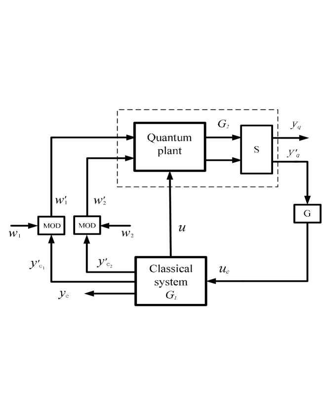
Figure 4: Feedback interconnection of a classical system $G_{1}$ and a quantum system $G_{2}$.

Proof: The proof consists of the following six steps.

Step 1. Construct the matrix $C^{\prime}_{c}$ satisfying Eq. (133). It follows from Eq. (77) with an invertible $\Theta_{y_{q}}$ that the matrix $D_{q}$ has full row rank and thus $\mathrm{rank}(\!D_{q}\!)\!=\!\mathrm{rank}\left(\![\begin{array}[]{cc}D_{q}\quad C_{qc}\\ \end{array}\!]\right)$. Consequently, the solution of Eq. (133) can be given as $C^{\prime}_{c}=D_{q}^{T}(D_{q}D_{q}^{T})^{-1}C_{qc}+N(D_{q})$, where $N(D_{q})$ denotes a matrix of the same dimension as $C^{\prime}_{c}$ whose columns are in the kernel space of $D_{q}$.

Step 2. Let

$$\bar{B}_{c}=B_{c}^{\prime}G,~{}~{}\bar{D}_{c}=D_{c}^{\prime}G.$$ (145)

Then Eqs. (135) and (137) can be re-written as

$$\left[\begin{array}[]{c}\bar{B}_{c}\\ \bar{D}_{c}\\ \end{array}\right]D^{\prime}_{q}=\left[\begin{array}[]{c}B_{c}\\ D_{c}\\ \end{array}\right].$$ (146)

We show that Eq. (146) has a solution $\left[\begin{array}[]{c}\bar{B}_{c}\\ \bar{D}_{c}\\ \end{array}\right]$. Combining Eqs. (78), (120) and (125) gives

$$\left[\begin{array}[]{c}D_{q}\\ D^{\prime}_{q}\\ \end{array}\right]\Theta_{w}(D^{\prime}_{q})^{T} = \left[\begin{array}[]{c}0_{2n_{y_{q}}\times(2m-2n_{y_{q}})}\\ \Theta_{y_{q}^{\prime}}\\ \end{array}\right],$$ (151)

$$\left[\begin{array}[]{c}D_{q}\\ D^{\prime}_{q}\\ \end{array}\right]\Theta_{w}\left[\begin{array}[]{cc}B_{c}^{T}\quad D_{c}^{T}\\ \end{array}\right] = \left[\begin{array}[]{c}0_{2n_{y_{q}}\times(n_{c}+n_{y_{c}})}\\ D^{\prime}_{q}\Theta_{w}\left[\begin{array}[]{cc}B_{c}^{T}&D_{c}^{T}\\ \end{array}\right]\\ \end{array}\right],$$ (158)

where $\Theta_{y_{q}^{\prime}}=\mathrm{diag}_{(m-n_{y_{q}})}(J)$. From equations (151) and (158), we can infer that $\mathrm{rank}\left((D^{\prime}_{q})^{T}\right)=\mathrm{rank}(\Theta_{y_{q}^{\prime}})$ , $\mathrm{rank}\left([\begin{array}[]{ccc}B_{c}^{T}\quad D_{c}^{T}\\ \end{array}]\right)=\mathrm{rank}\left(D^{\prime}_{q}\Theta_{w}[\begin{array}[]{cc}B_{c}^{T}\quad D_{c}^{T}\\ \end{array}]\right)$. Given that $\Theta_{y_{q}^{\prime}}$ has full row rank, we can conclude that $\mathrm{rank}\left(\Theta_{y_{q}^{\prime}}\right)=\mathrm{rank}\left(\left[\Theta_{y_{q}^{\prime}}\quad D^{\prime}_{q}\Theta_{w}[\begin{array}[]{cc}B_{c}^{T}\quad D_{c}^{T}\\ \end{array}]\right]\right)$, which implies that $\mathrm{rank}\left((D^{\prime}_{q})^{T}\right)=\mathrm{rank}\left(\left[\begin{array}[]{ccc}(D^{\prime}_{q})^{T}\quad B_{c}^{T}\quad D_{c}^{T}\\ \end{array}\right]\right)$. So, there exist $\bar{B}_{c}$ and $\bar{D}_{c}$ satisfying Eq. (146).

Step 3. We construct matrices $C^{\prime}_{c}$, $G$, and $B_{c}^{\prime}$. We get from equations (79), (119), (122), (135), (137), and (151) that

$$\left[\begin{array}[]{c}\bar{B}_{c}\\ \bar{D}_{c}\\ \end{array}\right]\Theta_{y_{q}^{\prime}}\left[\begin{array}[]{c}\bar{B}_{c}\\ \bar{D}_{c}\\ \end{array}\right]^{T}=0.$$ (163)

From equation (163), we know that the matrix $\left[\begin{array}[]{c}\bar{B}_{c}\\ \bar{D}_{c}\\ \end{array}\right]$ with $\mathrm{rank}\left(\left[\begin{array}[]{c}\bar{B}_{c}\\ \bar{D}_{c}\\ \end{array}\right]\right)=r$ can be decomposed as

$$\left[\begin{array}[]{c}\bar{B}_{c}\\ \bar{D}_{c}\\ \end{array}\right]=PZKV=\left[\begin{array}[]{c}P_{1}Z\\ P_{2}Z\\ \end{array}\right]KV,$$

where $P=\left[\begin{array}[]{c}P_{1}\\ P_{2}\\ \end{array}\right]$ is a permutation matrix; $Z$ is a matrix of the form $Z=\left[\begin{array}[]{c}I_{r}\\ X\\ \end{array}\right]$ if $r<n_{c}+n_{y_{c}}$, where $X$ is some $(n_{c}+n_{y_{c}}-r)\times r$ matrix, $Z=I_{(n_{c}+n_{y_{c}})}$ if $r=n_{c}+n_{y_{c}}$,

$$K=\left[\begin{array}[]{c}k_{1}\\ k_{2}\\ \vdots\\ k_{r}\end{array}\right]=\left[\begin{array}[]{cc}I_{r}&0_{r\times(n_{y_{q}^{\prime}}-r)}\end{array}\right]\in\mathbb{R}^{r\times n_{y_{q}^{\prime}}},$$ (164)

and $V$ is a symplectic matrix (see [31, Lemma 6] for details). Being symplectic, the matrix $V$ can be realized as a suitable static quantum optical network, [26]. We define

$$G=KV,\quad B_{c}^{\prime}=P_{1}Z,\quad D_{c}^{\prime}=P_{2}Z.$$ (165)

Step 4. From Eqs. (118), (123), and $C^{\prime}_{qq}$ defined in Eq. (132), we conclude that Eq. (135) implies Eq. (134), and Eq. 137 implies Eq. (136), respectively.

Step 5. It is straightforward to verify from Eqs. (133)-(144) that interconnecting the classical system $G_{1}$ and the quantum system $G_{2}$ gives the standard form (61)-(62), or equivalently described by (69)-(75). Now let us check that the system $G_{2}$ is a physically realizable fully quantum system. It follows from conditions (77) and (117) that the system $G_{2}$ satisfies constraints (100) and (102) in the sense of Theorem 3 with matrices $A$, $B$, $D$, $\Theta_{n}$ and $\mathrm{diag}(\Theta_{y_{q}},0_{n_{y_{c}}\times n_{y_{c}}})$ replaced by corresponding matrices $A_{qq}$, $B_{q}$, $D_{q}$, $\Theta_{n_{q}}$ and $\Theta_{y_{q}}$, respectively. The system $G_{2}$ also satisfies constraint (101) with its matrices replaced by corresponding matrices in equations (5)-(7) with the proof as follows:

$$-\Theta_{n_{q}}\left(\left[\begin{array}[]{c}D_{q}\\ D^{\prime}_{q}\\ \end{array}\right]\Theta_{w}B_{q}^{T}\Theta_{n_{q}}\right)^{T} = -\Theta_{n_{q}}\Theta_{n_{q}}^{T}B_{q}\Theta_{w}^{T}\left[\begin{array}[]{c}D_{q}\\ D^{\prime}_{q}\\ \end{array}\right]^{T}=B_{q}\Theta_{w}\left[\begin{array}[]{c}D_{q}\\ D^{\prime}_{q}\\ \end{array}\right]^{T}.$$

So, the system $G_{2}$ is a physically realizable quantum system, where $y_{q}^{\prime}$ is the input to the network G.

Step 6. By Eqs. (164) and (165), Applying $K$ to $Vy^{\prime}_{q}(t)$ is to measure the first $r$ amplitude quadrature components of $Vy^{\prime}_{q}(t)$ to obtain the measurement result $u_{c}(t)=KVy^{\prime}_{q}(t)=Gy^{\prime}_{q}(t)$. So, $G$ represents measurement processes, [31], [32]. Then we can show that

$$[u_{c}(t),~{}u_{c}(s)^{T}]=G[y_{q}^{\prime}(t),~{}y_{q}^{\prime}(s)^{T}]G^{T}=2i\delta_{ts}G\Theta_{y_{q}^{\prime}}G^{T}=2i\delta_{ts}\times 0=0,\forall t,s\geq 0,$$

which implies that $u_{c}$ is classical. Thus $G_{1}$ described by (5)-(7) is a classical system, where the classical vector signals $y^{\prime}_{c_{1}}(t)$ and $y^{\prime}_{c_{2}}(t)$ are used to modulate $w_{1}(t)$ and $w_{2}(t)$ to produce the quantum signals $w^{\prime}_{1}(t)$ and $w^{\prime}_{2}(t)$ which are then injected into $G_{2}$. $\blacksquare$

Remark 7

By Eqs. (143)-(144), we have

$$[dw^{\prime}_{1}(t),~{}dw^{\prime}_{2}(t)^{T}]=[dw_{1}(t),~{}dw_{2}(t)^{T}].$$

VI Application

When a system is described by a certain mathematical model, it is often important to perform some form of analysis on it. Our paper provides a mathematical means to convert a general representation of a mixed system to a standard form in which the system can be decomposed into two subsystems which make clear the quantum and classical components of the system. The main results of this paper may thus have a practical application in the analysis of measurement-based feedback control of quantum systems described by LSDEs, where the plant is a quantum system while the controller is a classical system [41], [18], [47], [44], [32]. This decomposition results in the mixed system with a more illuminating structure, making it easier to draw conclusions on the system’s quantum and classical subspaces. Then the quantum subsystem can be synthesized by quantum optical devices like beam splitters, phase shifters, optical cavities, squeezers, etc, and the classical subsystem can be built by standard analog or digital electronics; see [29], [43], [32]. Now an example is given to illustrate our main results.

$\mathbf{Example\ 2}$: Consider a mixed quantum-classical system of the standard form with $A,B,C,D$ satisfying the physical realizability conditions (100)-(102),

$$A=\left[\begin{array}[]{ccc}-9&-3&-1\\ 1&-7&-3\\ -0.72&-0.6&-12\\ \end{array}\right],\quad B=\left[\begin{array}[]{cccccc}1&2&-7&0&-3&5\\ 2&5&1&-3&6&-8\\ 0&0.12&0&0&0&-0.16\\ \end{array}\right],$$

$$C=\left[\begin{array}[]{ccc}38&46&-42\\ 0.31&0.4&0.35\\ 4.2&-6&5\\ \end{array}\right],\quad D=\left[\begin{array}[]{cccccc}8&0&10&0&6&0\\ 0&0.04&0&0.05&0&0.03\\ 0&0.8&0&-1&0&0.6\\ \end{array}\right].$$

Following the construction in the proof of Theorem 5, we have the classical system $G_{1}$ described by

$$dx_{c}(t) = -12x_{c}(t)+[3.6836\quad-0.4345]du_{c}(t),$$

$$dy_{c}(t) = 12x_{c}(t)dt+[-0.2065\quad 1.2388]du_{c}(t),$$

$$y_{c_{1}}^{\prime}(t) = 0,$$

$$y_{c_{2}}^{\prime}(t) = \left[\begin{array}[]{c}-4.2\\ 7\\ 0\\ 0\end{array}\right]x_{c}(t),$$

the quantum system $G_{2}$ given by

$$dx_{q}(t) = \left[\begin{array}[]{cc}-9&-3\\ 1&-7\\ \end{array}\right]x_{q}(t)dt\!+\!\left[\begin{array}[]{cc|cccc}1&2&-7&0&-3&5\\ 2&5&1&-3&6&-8\\ \end{array}\right]\!\!\left[\begin{array}[]{c}dw_{1}(t)\\ dw_{2}(t)\\ \end{array}\right]\!+\!\left[\begin{array}[]{c}-30.4\\ 22.2\\ \end{array}\right]du(t),$$

$$dy_{q}(t) = \left[\begin{array}[]{cc}38&46\\ 0.31&0.4\\ \end{array}\right]x_{q}(t)dt+\left[\begin{array}[]{cc|cccc}8&0&10&0&6&0\\ 0&0.04&0&0.05&0&0.03\\ \end{array}\right]\left[\begin{array}[]{c}dw_{1}(t)\\ dw_{2}(t)\\ \end{array}\right],$$

$$dy_{q}^{\prime}(t) = \left[\begin{array}[]{c}dy_{q_{1}}^{\prime}(t)\\ dy_{q_{2}}^{\prime}(t)\\ \end{array}\right]=\left[\begin{array}[]{cc}-1.1&2.3\\ 4.2&-6\\ -47&-14\\ -0.72&-0.6\\ \end{array}\right]x_{q}(t)dt\!+\!\left[\!\!\!\begin{array}[]{cc|cccc}0.4&0&-0.5&0&0.3&0\\ 0&0.8&0&-1&0&0.6\\ 3&0&0&0&-4&0\\ 0&0.12&0&0&0&-0.16\\ \end{array}\!\!\!\right]\left[\begin{array}[]{c}dw_{1}(t)\\ dw_{2}(t)\\ \end{array}\!\!\right],$$

and the matrix $G$ is given by

$$G\!=\!\left[\!\begin{array}[]{cccc}0&0.0971&0&0.2769\\ 0&0.8235&0&0.0462\\ \end{array}\!\right].$$

It can be easily checked that the closed-loop system described by (61)-(62) with the above matrices $A$, $B$, $C$, $D$ is obtained by making the identification

$$u(t) = x_{c}(t),$$

$$du_{c}(t) = \left[\begin{array}[]{cc}0.2086&-0.7489\\ 3.4253&-4.9684\\ \end{array}\right]x_{q}(t)dt+\!\!\left[\!\begin{array}[]{cc|cccc}0&0.1109&0&-0.0971&0&0.014\\ 0&0.6643&0&-0.8235&0&0.4867\\ \end{array}\!\right]\!\!\!\left[\begin{array}[]{c}dw_{1}(t)\\ dw_{2}(t)\\ \end{array}\right],$$

$$dw^{\prime}_{1}(t) = dw_{1}(t),$$

$$dw^{\prime}_{2}(t) = \left[\begin{array}[]{c}-4.2\\ 7\\ 0\\ 0\end{array}\right]x_{c}(t)dt\!+\!dw_{2}(t).$$

The realization of this mixed system is shown in Figure 5. The details of the construction and the individual components involved can be found in [23], [30], [43], [32] and the references therein.

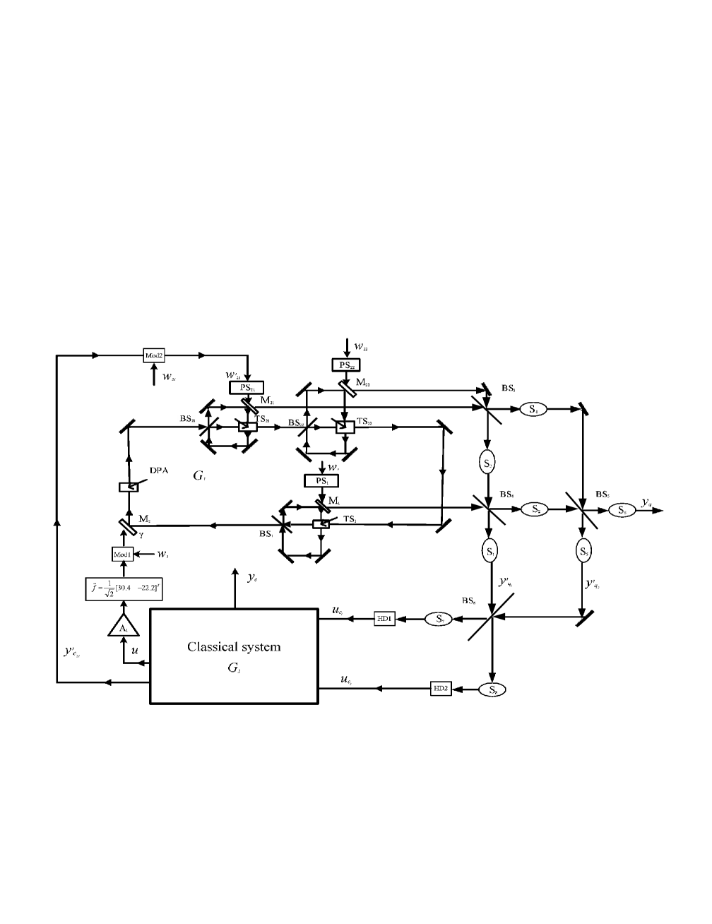
Figure 5: A realzation of the mixed quantum-classical system in Example 2. Black rectangles denote fully reflecting mirrors. $\mathrm{M_{1}},\mathrm{M_{21}},\mathrm{M_{22}}$ and $\mathrm{M_{3}}$ represent transmitting mirrors with coupling constants $\kappa_{1},\kappa_{21},\kappa_{22}$ and $\gamma$, respectively $(\gamma\ll 1,\gamma\ll\kappa_{1},\kappa_{21},\kappa_{22})$; $\mathrm{BS_{1}},\mathrm{BS_{21}},\mathrm{BS_{22}},\mathrm{BS_{3}},\mathrm{BS_{4}},\mathrm{BS_{5}}$ and $\mathrm{BS_{6}}$ represent beam splitters; $\mathrm{TS_{1}},\mathrm{TS_{21}}$ and $\mathrm{TS_{22}}$ represent two-mode squeezers; $\mathrm{PS_{1}}$, $\mathrm{PS_{21}}$, $\mathrm{PS_{22}}$ represent phase shifters; $\mathrm{S_{i}}$ $(i=1,2\cdots,8)$ represents a squeezer; DPA is short for degenerate parametric amplifier; $\mathrm{Modi}$ $(i=1,2,3,4)$ represents a modulator; $\mathrm{HDi}$ $(i=1,2)$ represents a homodyne detector; $\mathrm{A_{1}}$ is a amplifier with gain $1/\sqrt{\gamma}$. $\tilde{f}$ can be realized using a computer. $w_{1},w_{21},w_{22},w_{3}$ are vacuum noises and the contribution of $w_{3}$ to quantum system noise is negligible compared to that of other vacuum noises. $G_{2}$ can be realized by electrical and electronic devices, see [2].

VII Conclusion

In this paper, we explicitly detail how to obtain mathematical representations for a class of mixed quantum-classical linear stochastic systems; two forms (a standard form and a general form) are presented for the physical realization of such mixed systems. We have also established the relation between these two forms. Three physical realization constraints are derived for the standard form and the general form, respectively. A network theory is then developed for synthesizing linear dynamical mixed quantum-classical stochastic systems of the standard form in a systematic way. One feedback network architecture is proposed for this network realization.

References

• [1] D’Alessandro, D. (2007). Introduction to quantum control and dynamics. Chapman $\&$ Hall/CRC press.
• [2] Anderson, B. D. O., and Vongpanitlerd, S. (1973). Network analysis and synthesis: a modern systems theory approach. Networks Series, Prentice-Hall, Englewood Cliffs, NJ.
• [3] Accardi, L., Frigerio, A., and Lewis, J. T. (1982). Quantum stochastic processes. Publ. Res. Inst. Math. Sci., 18(1), 97-133.
• [4] Altafini, C., and Ticozzi, F. (2012). Modeling and control of quantum systems: An introduction. IEEE Trans. Automat. Control, 57(8), 1898-1917.
• [5] Bachor, H. A., and Ralph, T. C. (2004). A guide to experiments in quantum optics, 2nd Weinheim, Germany: Wiley-VCH.
• [6] Bouten, L., van Handel, R., and James, M. R. (2007). An introduction to quantum filtering. SIAM J. Control and Optimization, 46(6), 2199-2241.
• [7] Beausoleil, R. G., Keukes, P. J., Snider, G. S., Wang, S. Y., and Williams, R. S (2007). Nanoelectronic and nanophotonic interconnect. Proceedings of the IEEE, 96(2), 230-247.
• [8] Belavkin, V. P. (1991). Stochastic calculus of quantum input-output processes and quantum nondemolition filtering. J. of Soviet Mathematics, 56(5), 2625-2647, 1991.
• [9] Belavkin, V. P. (1994). Nondemolition principle of quantum measurement theory. Foundation of Physics, 24(5), 685-714.
• [10] Deotto, E., Gozzi, E., and Mauro, D (2003). Hilbert space structure in classical mechanics. I, II. J. Math. Phys., 44, 5902-5957.
• [11] Dong, D., and Petersen, I. (2010). Quantum control theory and applications: a survey. IET Control Theory $\&$ Applications, 4, 2651-2671.
• [12] Gardiner, C. W., and Collett, M. J. (1985). Input and output in damped quantum systems: Quantum stochastic differential equations and the master equation. Physical Review A, 31, 3761 C3774.
• [13] Accardi, L., Lu, Y. G., and Volovich, I. (2002). Quantum Theory and Its Stochastic Limit. Berlin Heidelberg: Springer.
• [14] Gardiner, C., and Zoller, P. (2004). Quantum noise, 3rd. Berlin, Germany: Springer.
• [15] Gough, J. E., and James, M. R. (2009). The series product and its application to quantum feedforward and feedback networks. IEEE Trans. Automatic Control, 54(11), 2530-2544.
• [16] Gough, J. E., James, M. R., and Nurdin, H. I. (2010). Squeezing components in linear quantum feedback networks. Phys. Rev. A, 81(2), 023804.
• [17] Gough, J. E. (2008). Construction of bilinear control Hamiltonians using the series product and quantum feedback. Phys. Rev. A, 78, 052311.
• [18] Gough, J. E.(2012). Principles and applications of quantum control engineering. Phil. Trans. R. Soc. A, 370, 5241-5258.
• [19] Gough, J. E. and Zhang, G. (2016) On realization theory of quantum linear systems, Automatica, 59, 139-151.
• [20] Hudson, R. L., and Parthasarathy, K. R. (1984). Quantum Ito’s formula and stochastic evolutions. Comm. Math. Phys., 93(3), 301-323.
• [21] Horn, R. A., and Johnson, C. R. (1985). Matrix Analysis, Cambridge University Press.
• [22] Jacobs, K. (2014). Quantum Measurement Theory and its Applications. Cambridge, UK: Cambridge University Press.
• [23] James, M. R., Nurdin, H. I., and Petersen, I. R. (2008). $H^{\infty}$ control of linear quantum stochastic systems. IEEE Trans. Automat. Control, 53, 1787-1803.
• [24] Kuang, S., and Cong. S. (2008) Lyapunov control methods of closed quantum systems. Automatica, 44(1), 98-108.
• [25] Leonhardt. U (2003). Quantum physics of simple optical instruments. Rep. Prog. Phys., 66, 1207’1249.
• [26] Leonhardt, U., and Neumaier, A. (2004). Explicit effective Hamiltonians for linear quantum-optical networks. J. Opt. B, 6, L1-L4.
• [27] Merzbacher, E. (1998). Quantum mechanics, 3rd. New York: Wiley.
• [28] Mirrahimi M., and van Handel, R. (2007) Stabilizing feedback controls for quantum systems. SIAM J. Control and Optim., 46, 445’467.
• [29] Nurdin, H.I., James, M.R., and Petersen, I. R. (2009). Coherent quantum LQG control. Automatica, 45, 1837-1846.
• [30] Nurdin, H. I., James, M. R., and Doherty, A. C. (2009). Network synthesis of linear dynamical quantum stochastic systems. SIAM J. Control and Optim., 48, 2686-2718.
• [31] Nurdin, H. I. (2011). Network synthesis of mixed quantum-classical linear stochastic systems. In Proceedings of the 2011 Australian Control Conference (AUCC), Engineers Australia, Australia, 68-75.
• [32] Nurdin H., and Yamamoto, N. (2017). Linear Dynamical Quantum Systems: Analysis, Synthesis, and Control. Springer, 2017.
• [33] Nielsen, S. and Kapral, R. (2001). Statistical mechanics of quantum-classical systems. J. of Chemical Phys., 115(13), 5805-5815.
• [34] Tsang, M. and Caves, C. (2012). Evading quantum mechanics: Engineering a classical subsystem within a quantum environment. Phys. Rev. X, 2, 031016.
• [35] O’Brien, J. L., Furusawa, A., and Vuckovic, J. (2009). Photonic quantum technologies. Nature Photonics, 3, 687-695.
• [36] Sayed Hassen, S.Z., Heurs, M., Huntington E.H., Petersen, I. R., and James, M. R. (2009). Frequency locking of an optical cavity using linear-quadratic Gaussian integral control, J. Phys. B: At. Mol. Opt. Phys., 42, 175501.
• [37] Shaiju, A. J., Petersen, I. R., and James, M. R. (2007). Guaranteed cost LQG control of uncertain linear stochastic quantum systems. In Proceedings of the 2007 American Control Conference, New York.
• [38] Ticozzi, F., and Viola, L., (2009). Analysis and synthesis of attractive quantum Markovian dynamics, Automatica 45, 2002-2009.
• [39] Wiseman, H. M., and Milburn, G. J. (1993). Quantum theory of optical feedback via homodyne detection. Phys. Rev. Lett., 70, 548-551.
• [40] Walls, D. F., and Milburn, G. J. (2008). Quantum Optics Springer-Verlag, New York.
• [41] Wiseman, H. M., and Milburn, G. J. (2010). Quantum Measurement and Control. Cambridge, UK: Cambridge University Press.
• [42] Wang, S., Nurdin, H. I., and Zhang, G. $\&$ James, R. M.(2012). Synthesis and structure of mixed quantum-classical linear systems. In Proceedings of the 51st IEEE Conference on Decision and Control (CDC), 1093-1098, Maui, Hawaii, USA.
• [43] Wang, S., Nurdin, H. I., Zhang, G., and James, R. M.(2013). Quantum optical realization of classical linear stochastic systems. Automatica, 49(10), 3090-3096.
• [44] Wilson, D. J., Sudhir, V., Piro, N., Schilling, R., Ghadimi, A., and Kippenberg, T. J. (2015). Measurement-based control of a mechanical oscillator at its thermal decoherence rate. Nature, 524, 325-329.
• [45] Xiang, C., Petersen, I. R., and Dong, D. Coherent robust H|finty control of linear quantum systems with uncertainties in the Hamiltonian and coupling operators. Automatica, 81, 8-21.
• [46] Yamamoto, N., Nurdin, H. I., James, M. R., and Petersen, I. R. (2008). Avoiding entanglement sudden death via measurement feedback control in a quantum network. Phys. Rev. A, 78, 042339.
• [47] Yamamoto, N. (2014). Coherent versus Measurement Feedback: Linear Systems Theory for Quantum Information. Phys. Rev. X, 4(4), 041029.
• [48] Zhang, G., and James M. R. (2011). Direct and indirect couplings in coherent feedback control of linear quantum systems. IEEE Trans. Automat. Contr., 56(7), 1535-1550.
• [49] Zhang, G., and James, M. R. (2012). Quantum feedback networks and control: a brief survey. Chinese Science Bulletin, 57, 2200-2214.
• [50] Zhang, J., Liu, Y-X., Wu, R-B., Jacobs, K., and Nori. F. (2017). Quantum feedback: theory, experiments, and applications. Physics Reports, 679, 1-60.
• [51] Zhang, G., Grivopoulos, S., Petersen, I. R., and Gough, J. E. (2018), The Kalman decomposition for linear quantum systems, IEEE Trans. Automat. Contr., 63(2), 331-346.