On a Theorem by Bojanov and Naidenov applied to families of Gegenbauer-Sobolev polynomials

Abstract.

Let $\{Q^{(\alpha)}_{n,\lambda}\}_{n\geq 0}$ be the sequence of monic orthogonal polynomials with respect the Gegenbauer-Sobolev inner product

$$\langle f,g\rangle_{S}:=\int_{-1}^{1}f(x)g(x)(1-x^{2})^{\alpha-\frac{1}{2}}dx+\lambda\int_{-1}^{1}f^{\prime}(x)g^{\prime}(x)(1-x^{2})^{\alpha-\frac{1}{2}}dx,$$

where $\alpha>-\frac{1}{2}$ and $\lambda\geq 0$. In this paper we use a recent result due to B.D. Bojanov and N. Naidenov [3], in order to study the maximization of a local extremum of the $k$th derivative $\frac{d^{k}}{dx^{k}}Q^{(\alpha)}_{n,\lambda}$ in $[-M_{n,\lambda},M_{n,\lambda}]$, where $M_{n,\lambda}$ is a suitable value such that all zeros of the polynomial $Q^{(\alpha)}_{n,\lambda}$ are contained in $[-M_{n,\lambda},M_{n,\lambda}]$ and the function $\left|Q^{(\alpha)}_{n,\lambda}\right|$ attains its maximal value at the end-points of such interval. Also, some illustrative numerical examples are presented.

Key words and phrases: Sobolev orthogonal polynomials; oscillating polynomials.

1. Introduction

Extremal properties for general orthogonal polynomials is an interesting subject in approximation theory and their applications permeate many fields in science and engineering [5, 18, 21, 28, 29]. Although it may seem an old subject from the view point of the standard orthogonality [5, 18, 29], this is not the case neither in the general setting (cf. [11, 12, 13, 14, 20]) nor from the view point of Sobolev orthogonality, where it remains like a partially explored subject [1]. In fact, new results continue to appear in some recent publications [10, 11, 12, 24, 26, 27].

Let $d\mu(x)=(1-x^{2})^{\alpha-\frac{1}{2}}dx$ with $\alpha>-\frac{1}{2}$, be the Gegenbauer measure supported on the interval $[-1,1]$. We consider the following Sobolev inner product on the linear space $\mathbb{P}$ of polynomials with real coefficients.

(1.1) $$\langle f,g\rangle_{S}:=\int_{-1}^{1}f(x)g(x)d\mu(x)+\lambda\int_{-1}^{1}f^{\prime}(x)g^{\prime}(x)d\mu(x),$$

where $\lambda\geq 0$. Let $\{Q^{(\alpha)}_{n,\lambda}\}_{n\geq 0}$ denote the sequence of monic orthogonal polynomials with respect to (1.1). These polynomials are usually called monic Gegenbauer-Sobolev polynomials [7, 8, 15, 16, 17, 25] and it is known that the zeros of these polynomials are in the real line [15, 16], and therefore they belong to other important class of algebraic polynomials, namely the oscillating polynomials [3, 19].

The main result of [3] allows to guarantee the maximal absolute value of higher derivatives of a symmetric oscillating polynomial on a finite interval are attained in the end-points of such interval, whenever the maximal absolute value of the polynomial is attained in the end-points of that interval. Then, [3, Section 4] contains a brief explanation about applications of previous result to orthogonal polynomials on the real line associated to symmetric weights. We focus our attention on that last part of [3, Section 4] in order to enlarge the range of application of [3, Theorem 1] to the class of Gegenbauer-Sobolev polynomials corresponding to the inner product (1.1).

The paper is structured as follows. Section 2 provides some background about structural properties of the Gegenbauer and Gegenbauer-Sobolev polynomials corresponding to the inner product (1.1), respectively. Section 3 contains some well-known characteristics of the class of oscillating polynomials on a finite interval. We also state there our main result (see Theorem 3.2) and provide some illustrative numerical examples. Throughout this paper, the notation $u_{n}\cong v_{n}$ means that the sequence $\left\{\frac{u_{n}}{v_{n}}\right\}_{n}$ converges to $1$ as $n\rightarrow\infty$. We will denote by $\mathbb{P}_{n}$ and $\|f\|_{\infty}$, the space of polynomials of degree at most $n$ and the uniform norm of $f$ on the interval in consideration, respectively. Any other standard notation will be properly introduced whenever needed.

2. Basic facts: Gegenbauer and Gegenbauer-Sobolev orthogonal polynomials

For $\alpha>-\frac{1}{2}$ we denote by $\{\hat{C}^{(\alpha)}_{n}\}_{n\geq 0}$ the sequence of Gegenbauer polynomials, orthogonal on $[-1,1]$ with respect to the measure $d\mu(x)$ (cf. [29, Chapter IV]), normalized by

$$\hat{C}^{(\alpha)}_{n}(1)=\frac{\Gamma(n+2\alpha)}{n!\Gamma(2\alpha)}.$$

It is clear that this normalization does not allow $\alpha$ to be zero or a negative integer. Nevertheless, the following limits exist for every $x\in[-1,1]$ (see [29, formula (4.7.8)].)

$$\lim_{\alpha\to 0}\hat{C}^{(\alpha)}_{0}(x)=T_{0}(x),\quad\lim_{\alpha\to 0}\frac{\hat{C}^{(\alpha)}_{n}(x)}{\alpha}=\frac{2}{n}T_{n}(x),$$

where $T_{n}$ is the $n$th Chebyshev polynomial of the first kind. In order to avoid confusing notation, we define the sequence $\{\hat{C}^{(0)}_{n}\}_{n\geq 0}$ as follows.

$$\hat{C}^{(0)}_{0}(1)=1,\quad\hat{C}^{(0)}_{n}(1)=\frac{2}{n},\quad\hat{C}^{(0)}_{n}(x)=\frac{2}{n}T_{n}(x),\quad n\geq 1.$$

We denote the $n$th monic Gegenbauer orthogonal polynomial by

(2.2) $$C^{(\alpha)}_{n}(x)=(h^{\alpha}_{n})^{-1}\hat{C}^{(\alpha)}_{n}(x),$$

where the constant $h^{\alpha}_{n}$ (cf. [29, formula (4.7.31)]) is given by

(2.3) $$h^{\alpha}_{n} = \frac{2^{n}\Gamma(n+\alpha)}{n!\Gamma(\alpha)},\quad\alpha\not=0,$$

(2.4) $$h^{0}_{n} = \lim_{\alpha\to 0}\frac{h^{\alpha}_{n}}{\alpha}=\frac{2^{n}}{n},\quad n\geq 1.$$

Then for $n\geq 1$, we have $C^{(0)}_{n}(x)=\lim_{\alpha\to 0}(h^{\alpha}_{n})^{-1}\hat{C}^{(\alpha)}_{n}(x)=\frac{1}{2^{n-1}}T_{n}(x)$.

Proposition 2.1.

Let $\{C^{(\alpha)}_{n}\}_{n\geq 0}$ be the sequence of monic Gegenbauer orthogonal polynomials. Then the following statements hold.

1. Three-term recurrence relation. For every $n\in\mathbb{N}$,

   (2.5) $$xC^{(\alpha)}_{n}(x)=C^{(\alpha)}_{n+1}(x)+\gamma_{n}^{(\alpha)}C^{(\alpha)}_{n-1}(x),\quad\alpha>-\frac{1}{2},\quad\alpha\not=0,$$

   with initial conditions $C^{(\alpha)}_{0}(x)=1$, $C^{(\alpha)}_{1}(x)=x$, and recurrence coefficient $\gamma_{n}^{(\alpha)}=\frac{n(n+2\alpha-1)}{4(n+\alpha)(n+\alpha-1)}$.

2. For every $n\in\mathbb{N}$ (see [29, formula (4.7.15)]),

   (2.6) $$\|C^{(\alpha)}_{n}\|_{\mu}^{2}=\int_{-1}^{1}[C^{(\alpha)}_{n}(x)]^{2}d\mu(x)=\pi 2^{1-2\alpha-2n}\frac{n!\Gamma(n+2\alpha)}{\Gamma(n+\alpha+1)\Gamma(n+\alpha)}.$$

3. Structure relation (see [29, formula (4.7.29)]). For every $n\geq 2$,

   (2.7) $$C^{(\alpha-1)}_{n}(x)=C^{(\alpha)}_{n}(x)+\xi_{n-2}^{(\alpha)}C^{(\alpha)}_{n-2}(x),$$

   where

   (2.8) $$\xi_{n}^{(\alpha)}=\frac{(n+2)(n+1)}{4(n+\alpha+1)(n+\alpha)},\quad n\geq 0.$$

4. For every $n\in\mathbb{N}$ (see [29, formula (4.7.14)]),

   (2.9) $$\frac{d}{dx}C^{(\alpha)}_{n}(x)=nC^{(\alpha+1)}_{n-1}(x).$$

Some well-known properties of the monic Gegenbauer-Sobolev orthogonal polynomials corresponding to the inner product (1.1) are the following.

Proposition 2.2.

Let $\{Q^{(\alpha)}_{n,\lambda}\}_{n\geq 0}$ be the sequence of monic orthogonal polynomials with respect to (1.1). Then the following statements hold.

1. The polynomials $Q^{(\alpha)}_{n,\lambda}$ are symmetric, i.e.,

   (2.10) $$Q^{(\alpha)}_{n,\lambda}(-x)=(-1)^{n}Q^{(\alpha)}_{n,\lambda}(x).$$

2. The zeros of $Q^{(\alpha)}_{n,\lambda}$ are real and simple, and they interlace with the zeros of the monic Gegenbauer orthogonal polynomials $C^{(\alpha)}_{n}$. Furthermore, for $\alpha\geq\frac{1}{2}$ they are all contained in the interval $[-1,1]$ and for $-\frac{1}{2}<\alpha<\frac{1}{2}$ there is at most a pair of zeros symmetric with respect to the origin outside the interval $[-1,1]$, (cf. [15, 16]).

3. [15, Lemma 5.1]. For $\alpha\geq\frac{1}{2}$, we have $Q^{(\alpha)}_{n,\lambda}(1)>0$.

It is worthwhile to point out that in the case $-\frac{1}{2}<\alpha<\frac{1}{2}$, no global properties about the sign $Q^{(\alpha)}_{n,\lambda}(1)$ can be deduced (cf. [15].)

However, the location of zeros of Sobolev orthogonal polynomials is not a trivial problem. For instance, if we consider $(\mu_{0},\mu_{1})$ a vector of compactly supported positive measures on the real line with finite total mass and the following Sobolev inner product on the linear space $\mathbb{P}$ of polynomials with real coefficients.

(2.11) $$\langle f,g\rangle_{(\mu_{0},\mu_{1})}:=\int f(x)g(x)d\mu_{0}(x)+\int f^{\prime}(x)g^{\prime}(x)d\mu_{1}(x),$$

then, simple examples show that the zeros of these Sobolev orthogonal polynomials do not necessarily remain in the convex hull of the union of the supports of the measures $\mu_{k}$, $k=0,1$, and they can be complex. In this regard some numerical experiments may be found in [9]. In particular, the boundedness of the zeros of Sobolev orthogonal polynomials is an open problem [1, 16], but as was stated in [10], it could be obtained as a consequence of the boundedness of the multiplication operator $Mf(z)=zf(z)$: If $M$ is bounded and $\|M\|$ is its operator norm (induced by (2.11)), then all the zeros of the Sobolev orthogonal polynomials $Q_{n}$ are contained in the disc $\{z\in\mathbb{C}:|z|\leq\|M\|\}$.

Indeed, if $x_{0}$ is a zero of $Q_{n}$ then $xp(x)=x_{0}p(x)+Q_{n}(x)$ for a polynomial $p\in\mathbb{P}_{n-1}$. Since $p$ and $Q_{n}$ are orthogonal, we get

$$|x_{0}|^{2}\|p\|_{(\mu_{0},\mu_{1})}^{2}=\|xp\|^{2}_{(\mu_{0},\mu_{1})}-\|Q_{n}\|^{2}_{(\mu_{0},\mu_{1})}\leq\|xp\|_{(\mu_{0},\mu_{1})}^{2}=\|Mp\|_{(\mu_{0},\mu_{1})}^{2}\leq\|M\|^{2}\|p\|_{(\mu_{0},\mu_{1})}^{2},$$

which yields the above result.

Thus, in the last decades the question whether or not the multiplication operator $M$ is bounded has been a topic of interest to investigators in the field, since it turns out to be a key for the location of zeros and for establishing the asymptotic behavior of orthogonal polynomials with respect to diagonal (or non-diagonal) Sobolev inner products (cf. [16, 26, 27] and the references therein)

From the structure relation (2.7) and [17, formula (3)] (see also [7, Proposition 1]) the following connection formula can be obtained.

Proposition 2.3.

For $\alpha>-\frac{1}{2}$,

(2.12) $$C^{(\alpha-1)}_{n}(x)=Q^{(\alpha)}_{n,\lambda}(x)-d_{n-2}(\alpha)Q^{(\alpha)}_{n-2,\lambda}(x),\quad n\geq 2,$$

where

(2.13) $$d_{n}(\alpha)=\xi^{(\alpha)}_{n}\frac{\|C^{(\alpha)}_{n}\|_{\mu}^{2}}{\|Q^{(\alpha)}_{n,\lambda}\|_{S}^{2}}.$$

Moreover,

(2.14) $$d_{n}(\alpha)\cong\frac{1}{16\lambda n^{2}}.$$

3. Maximization of local extremum of the derivatives for families of Gegenbauer-Sobolev polynomials

A polynomial $P\in\mathbb{P}$ is said oscillating (see [2, 3, 4, 19, 22, 23]) if it has all its zeros on the real line $\mathbb{R}$. For example, the classical orthogonal polynomials on subsets of $\mathbb{R}$ (Hermite, Laguerre and Jacobi polynomials [6, 20, 29]), orthogonal polynomials for weights in the Nevai class $M(0,1)$ [21], including whose orthogonal with respect to weights belonging to Levin-Lubinsky class $\hat{\mathcal{W}}$ [13], and a broad class of Sobolev orthogonal polynomials [7, 9, 15, 16, 17, 25] constitute an important family of oscillating polynomials. Usually, when all zeros of a polynomial $P\in\mathbb{P}_{n}$ with $\deg(P)=n$, are contained in a given finite interval $[a,b]$, it is called oscillating polynomial on $[a,b]$, (see [3, 19].)

We denote by ${\rm Osc}(\mathbb{R})$ and ${\rm Osc}[a,b]$ the classes of oscillating polynomials on $\mathbb{R}$ and $[a,b]$, respectively. For any $P\in{\rm Osc}[a,b]$ with $\deg(P)=n$, we consider the vector ${\bf h}(P)=(h_{0}(P),\ldots,h_{n}(P))$, where $h_{j}(P)=|P(t_{j})|$, $0\leq j\leq n$, $t_{0}=a$, $t_{n}=b$, and $t_{1}\leq t_{2}\leq\cdots\leq t_{n-1}$ are the zeros of $P^{\prime}$.

Amongst the main characteristics of the class ${\rm Osc}[a,b]$ we list the following.

1. $P^{\prime}\in{\rm Osc}[a,b]$, for all $P\in{\rm Osc}[a,b]$.

2. Any $P\in{\rm Osc}[a,b]$ is completely determined by its local extrema and the values at the end-points of the interval $[a,b]$ (cf. [2, Theorem 2], [4, Remark 1].)

3. For $P\in{\rm Osc}[a,b]$ with $\deg(P)=n$, there exists a monotone dependence of the parameters $h_{j}(P^{\prime})$ on the parameters $h_{0}(P),\ldots,h_{n}(P)$ of $P$ (cf. [4, Lemma 3].)

4. If $P\in{\rm Osc}[a,b]$ with $\deg(P)\geq 3$ and $\|P\|=|P(a)|$, then each local extremum of $P^{\prime}$ from the first half (i.e., with an index less than or equal to $\left\lfloor\frac{n-1}{2}\right\rfloor$, and $\lfloor t\rfloor$ denoting the integer part of $t$) is smaller in absolute value than $|P^{\prime}(a)|$.

More precisely, the property iv) was stated in the following theorem.

Theorem 3.1.

([3, Theorem 1]) Let $P\in{\rm Osc}[a,b]$ with $\deg(P)\geq 3$. Assume that $\|P\|_{\infty}=|P(a)|=1$. Then

(3.15) $$|P^{\prime}(\tau_{j})|<|P^{\prime}(a)|,\mbox{ for }j=0,\ldots,\left\lfloor\frac{n-1}{2}\right\rfloor,$$

where $\tau_{1}\leq\cdots\leq\tau_{n-2}$ are the zeros of $P^{\prime\prime}$.

Corollary 3.1.

([3, Corollary 1]) Let $P\in{\rm Osc}[-1,1]$ be a symmetric polynomial, with $\deg(P)=n$. Assume that $\|P\|_{\infty}=|P(1)|=1$. Then,

(3.16) $$\|P^{(k)}\|_{\infty}=|P^{(k)}(1)|,\,\mbox{ for }k=1,\ldots,n.$$

As a consequence of the combination of Theorem 3.1 (or Corollary 3.1) and the structural properties of the sequence $\{Q^{(\alpha)}_{n,\lambda}\}_{n\geq 0}$ given in the previous section, we can obtain the maximization of local extremum of the derivatives for the sequence $\{Q^{(\alpha)}_{n,\lambda}\}_{n\geq 0}$ as follows.

Let $\{Q^{(\alpha)}_{n,\lambda}\}_{n\geq 0}$ be the sequence of monic orthogonal polynomials with respect to (1.1). Let us consider $x_{n,\lambda}^{\alpha,[1]}<x_{n,\lambda}^{\alpha,[2]}<\cdots<x_{n,\lambda}^{\alpha,[n]}$ the zeros of the Gegenbauer-Sobolev polynomial $Q^{(\alpha)}_{n,\lambda}$ and $N$ the maximum value attained by $|Q^{(\alpha)}_{n,\lambda}(x)|$ on the interval $[x_{n,\lambda}^{\alpha,[1]},x_{n,\lambda}^{\alpha,[n]}]$. Then $M_{n,\lambda}$ can be defined to be the minimal real point such that $x_{n,\lambda}^{\alpha,[n]}<M_{n,\lambda}$ and $|Q^{(\alpha)}_{n,\lambda}(M_{n,\lambda})|=N$, i.e., $M_{n,\lambda}$ is the point closest to $x_{n,\lambda}^{\alpha,[n]}$ where the maximal absolute value of the polynomial $Q^{(\alpha)}_{n,\lambda}$ is attained. Notice that $M_{n,\lambda}$ also depends on the parameter $\alpha$ and $Q^{(\alpha)}_{n,\lambda}\in{\rm Osc}[-M_{n,\lambda},M_{n,\lambda}]$. Thus, we can consider the following normalized polynomials

(3.17) $$q^{(\alpha)}_{n,\lambda}(x):=\frac{Q^{(\alpha)}_{n,\lambda}(x)}{Q^{(\alpha)}_{n,\lambda}(M_{n,\lambda})},\quad x\in[-M_{n,\lambda},M_{n,\lambda}],\quad n\geq 0.$$

Theorem 3.2.

Let $\{q^{(\alpha)}_{n,\lambda}\}_{n\geq 0}$ be the sequence of orthogonal polynomials given in (3.17). Then $\left|\frac{d^{k}}{dx^{k}}q^{(\alpha)}_{n,\lambda}\right|$ attains its maximal value on the interval $[-M_{n,\lambda},M_{n,\lambda}]$ at the end-points, for $\alpha>-\frac{1}{2}$ and $1\leq k\leq n$.

Proof.

It suffices to follow the proof of Theorem 3.1 (or Corollary 3.1) given in [3, Theorem 1 (or Corollary 1)] by making the corresponding modifications. ∎

Notice that from a numerical point of view the value $M_{n,\lambda}$ can be difficult to obtain for $n$ large enough. However, for any value $K>0$ such that $N<|Q^{(\alpha)}_{n,\lambda}(x)|$ for $x<-K$ and $x>K$, the result of Theorem 3.2 remains true on the interval $[-K,K]$.

We finish this section providing some illustrative numerical examples (with the help of MAPLE) about the above result for different values of $n$, $\alpha$ and $\lambda$ (see Figure 1 and Figure 2 below).

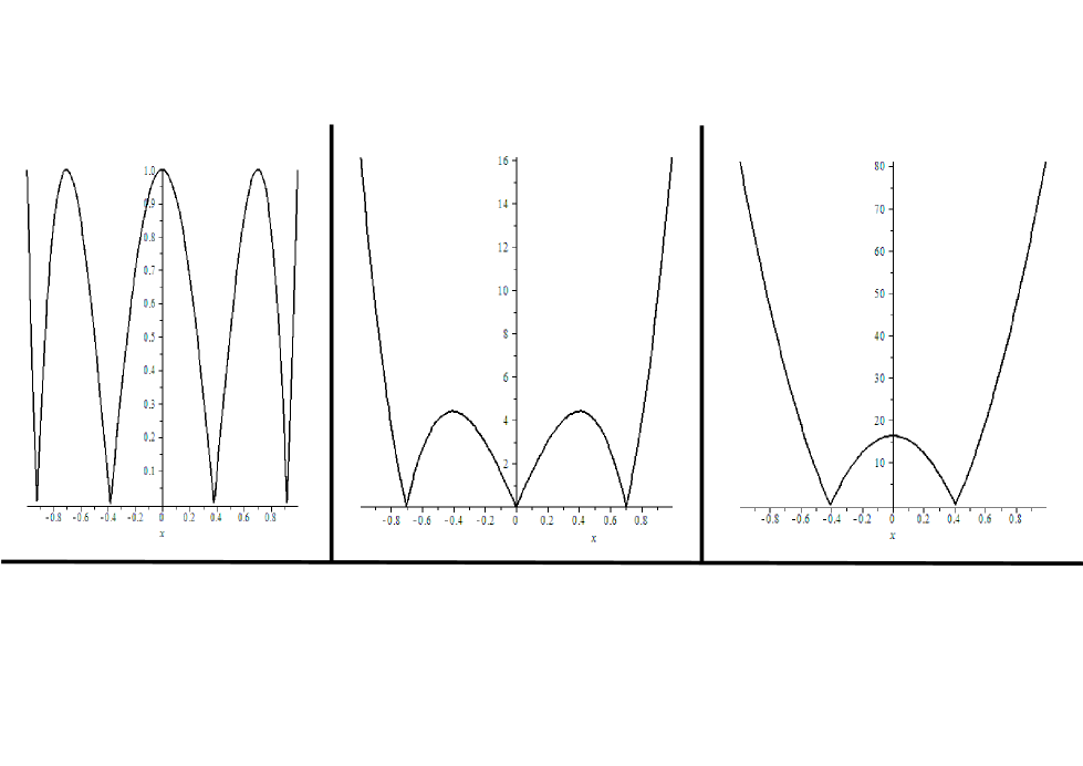
Figure 1. Graphics of $|\frac{d^{k}}{dx^{k}}q^{(\alpha)}_{n,\lambda}|$ for $n=4$, $\alpha=\lambda=1$, $M_{n,\lambda}=0.9926198253$ and $k=0,1,2$, respectively.

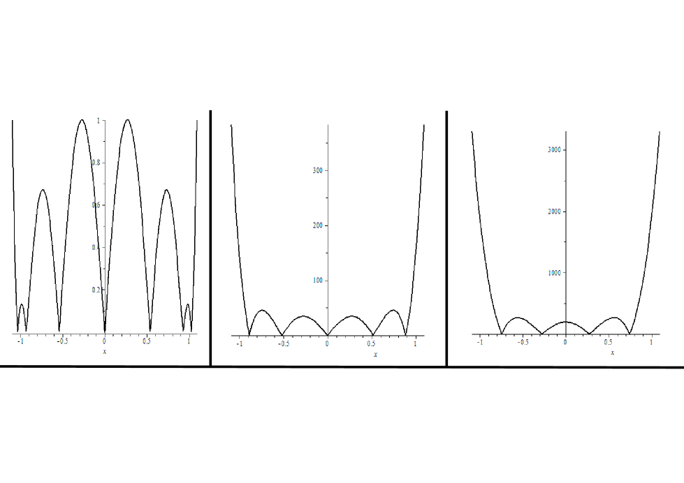
Figure 2. Graphics of $|\frac{d^{k}}{dx^{k}}q^{(\alpha)}_{n,\lambda}|$ for $n=7$, $\alpha=-\frac{1}{4}$, $\lambda=\frac{1}{2}$, $M_{n,\lambda}=1.091516326$ and $k=0,2,3$, respectively.

Acknowledgments.

The authors would like to express their gratitude to Professors D.K. Dimitrov and G. Nikolov for providing them some helpful academic materials and guidance during the preparation of this manuscript.

References

- [1] I. Baratchart, A. Martínez-Finkelshtein, D. Jiménez, D.S. Lubinsky, H.N. Mhaskar, I. Pritsker, M. Putinar, M. Stylianopoulus, V. Totik, P. Varju, Y. Xu, Open problems in Constructive Function Theory, Electron. Trans. Numer. Anal. 25 (2006), 511–525.
- [2] B.D. Bojanov, A generalization of Chebyshev polynomials, J. Approx. Theory 26 (1979), 293–300.
- [3] B.D. Bojanov, N. Naidenov, On oscillating polynomials, J. Approx. Theory 162 (2010), 1766–1787.
- [4] B.D. Bojanov, Q.I. Rahman, On certain extremal problems for polynomials, J. Math. Anal. Appl. 189 (1995), 781–800.
- [5] P. Borwein and T. Erdélyi, Polynomials and Polynomials Inequalities. Springer-Verlag, New York, EEUU, 1995.
- [6] D.K. Dimitrov, A late report on Interlacing of zeros of polynomials, Proc. Constructive Theory of Functions, Sozopol 2010. In memory of Borislav Bojanov, G. Nikolov and R. Uluchev (Eds.), 69–79. Prof. Marin Drinov Academic Publishing House, Sofia, 2012.
- [7] B. Xh. Fejzullahu, Asymptotic properties and Fourier expansions of orthogonal polynomials with a non-discrete Gegenbauer-Sobolev inner product, J. Approx. Theory 162 (2010), 397–406.
- [8] B.Xh. Fejzullahu, A Cohen type inequality for Fourier expansions of orthogonal polynomials with a non-discrete Gegenbauer-Sobolev inner product, Math. Nachr. 284 (2011), 24–254.
- [9] W. Gautschi, A.B.J. Kuijlaars, Zeros and critical points of Sobolev orthogonal polynomials, J. Approx. Theory 91 (1997), 117–137.
- [10] G. López-Lagomasino, I. Pérez-Izquierdo, H. Pijeira-Cabrera , Sobolev orthogonal polynomials in the complex plane, J. Comput. Appl. Math. 127 (2001), 219–230.
- [11] G. López-Lagomasino, I. Pérez-Izquierdo, H. Pijeira, Asymptotic of extremal polynomials in the complex plane, J. Approx. Theory 137 (2005), 226–237.
- [12] D.S. Lubinsky, A survey of weighted polynomial approximation with exponential weights, Surveys in Approximation Theory, 3 (2007), 1–105.
- [13] A.L. Levin, D.S. Lubinsky, Christoffel Functions and Orthogonal Polynomials for exponential weights on , Mem. Amer. Math. Soc. Vol. 111 (535) Amer. Math. Soc. Providence, RI (1994).
- [14] E. Levin, D.S. Lubinsky, Orthogonal polynomials for exponential weights, Springer-Verlag, New York, 2001.
- [15] F. Marcellán, T.E. Pérez, M.A. Piñar, Gegenbauer-Sobolev orthogonal polynomials in A. Cuyt (Ed.), Proc. Conf. on Nonlinear Numerical Methods and Rational Approximation II, Kluwer Academic Publishers, Dordrecht, 1994. 71-82.
- [16] A. Martínez-Finkelshtein, Analytic aspects of Sobolev orthogonal polynomials revisited, J. Comp. Appl. Math. 127 (2001), 255–266.
- [17] A. Martínez-Finkelshtein, J.J. Moreno-Balcázar, H. Pijeira-Cabrera, Strong asymptotics for Gegenbauer-Sobolev orthogonal polynomials, J. Comp. Appl. Math. 81 (1997), 211–216.
- [18] G.V. Milovanović, D.S. Mitrinović, Th.M. Rassias: Topics in Polynomials: Extremal problems, inequalities, zeros, Wordl Scientific Publishing Co. Pte. Ltd., Singapore, 1994.
- [19] N. Naidenov, Estimates for the derivatives of oscillating polynomials, East Journal on Approximations, 11 (3) (2005), 301–336.
- [20] P. Nevai, Géza Freud, Orthogonal Polynomials and Christoffel Functions. A Case Study. Journal of Approximation Theory, 48 (1986), 3–167.
- [21] P. Nevai, Orthogonal Polynomials, Mem. Amer. Math. Soc. Vol. 18 (213) Amer. Math. Soc. Providence, RI (1979).
- [22] G. Nikolov, Inequalities of Duffin-Schaeffer type, SIAM J. Math. Anal. 33 (3) (2001), 686–698.
- [23] G. Nikolov, An extension of an inequality of Duffin and Schaeffer, Constr. Approx. 21 (2005), 181–191.
- [24] D. Pérez, Y. Quintana, Some Markov-Bernstein type inequalities and certain class of Sobolev polynomials. J. Adv. Math. S. 4 (2011), 85–100.
- [25] H. Pijeira, Y. Quintana, W. Urbina, Zero location and asymptotic behavior of orthogonal polynomials of Jabobi-Sobolev, Rev. Col. Mat. 35 (2001), 77–97.
- [26] A. Portilla, Y. Quintana, J. M. Rodríguez, E. Tourís, Zero location and asymptotic behavior for extremal polynomials with non-diagonal Sobolev norms, J. Approx. Theory 162 (2010), 2225–2242.
- [27] A. Portilla, Y. Quintana, J. M. Rodríguez, E. Tourís, Concerning asymptotic behavior for extremal polynomials associated to non-diagonal Sobolev norms, J. Funct. Spaces Appl. 2013, article ID 628031 (2013), 1–11.
- [28] H. Stahl, V. Totik, General Orthogonal Polynomials, Cambridge University Press, Cambridge (1992).
- [29] G. Szegő, Orthogonal Polynomials, Coll. Publ. Amer. Math. Soc. Vol. 23, (4th ed.), Amer. Math. Soc. Providence, RI (1975).