Convergence of Markovian Stochastic Approximation with discontinuous dynamics

Abstract

This paper is devoted to the convergence analysis of stochastic approximation algorithms of the form $\theta_{n+1}=\theta_{n}+\gamma_{n+1}H_{\theta_{n}}(X_{n+1})$ where $\left\{\theta_{n},n\in\mathbb{N}\right\}$ is a $\mathbb{R}^{d}$-valued sequence, $\left\{\gamma_{n},n\in\mathbb{N}\right\}$ is a deterministic step-size sequence and $\left\{X_{n},n\in\mathbb{N}\right\}$ is a controlled Markov chain. We study the convergence under weak assumptions on smoothness-in-$\theta$ of the function $\theta\mapsto H_{\theta}(x)$. It is usually assumed that this function is continuous for any $x$; in this work, we relax this condition. Our results are illustrated by considering stochastic approximation algorithms for (adaptive) quantile estimation and a penalized version of the vector quantization.

siconxxxxxxxx–x

1 Introduction

Stochastic Approximation (SA) methods have been introduced by [35] as algorithms to find the roots of $h:\Theta\to\mathbb{R}^{d}$ where $\Theta$ is an open subset of $\mathbb{R}^{d}$ (equipped with its Borel $\sigma$-field $\mathcal{B}(\Theta)$) when only noisy measurements of $h$ are available. More precisely, let $\mathsf{X}$ be a space equipped with a countably generated $\sigma$-field $\mathcal{X}$, $\{P_{\theta},\theta\in\Theta\}$ be a family of transition kernels on $(\mathsf{X},\mathcal{X})$ and $H:\mathsf{X}\times\Theta\to\mathbb{R}^{d}$, $(x,\theta)\mapsto H_{\theta}(x)$ be a measurable function. We consider

$$\theta_{n+1}=\theta_{n}+\gamma_{n+1}H_{\theta_{n}}(X_{n+1})$$ (1)

where $\left\{\gamma_{n},n\in\mathbb{N}\right\}$ is a sequence of deterministic nonnegative step sizes and $\left\{X_{n},n\in\mathbb{N}\right\}$ is a controlled Markov chain, i.e., for any non-negative measurable function $f$,

$$\mathbb{E}[f(X_{n+1})|\mathcal{F}_{n}]=P_{\theta_{n}}f(X_{n}),\quad\mathbb{P}-\mathrm{a.s.}\ ,\quad\mathcal{F}_{n}=\sigma((X_{\ell},\theta_{\ell}),\ell\leq n).$$

It is assumed that for each $\theta\in\Theta$, $P_{\theta}$ admits a unique stationary distribution $\pi_{\theta}$ and that $h(\theta)=\int_{\mathsf{X}}H_{\theta}(x)\pi_{\theta}(\mathrm{d}x)=\pi_{\theta}(H_{\theta})$ (assuming that $\pi_{\theta}(|H_{\theta}|)<\infty$). This setting encompasses the cases $\left\{X_{n},n\in\mathbb{N}\right\}$ is a (non-controlled) Markov chain by choosing $P_{\theta}=P$ for any $\theta$; the Robbins-Monro case by choosing $P_{\theta}(x,\cdot)=\pi_{\theta}(\cdot)$ where $\pi_{\theta}$ is a distribution on $\mathsf{X}$; the case when $\left\{X_{n},n\in\mathbb{N}\right\}$ is an i.i.d. sequence with distribution $\pi$ by choosing $P_{\theta}(x,\cdot)=\pi(\cdot)$ for any $x,\theta$.

The goal of this paper is to provide almost sure convergence results of the sequence $\left\{\theta_{n},n\in\mathbb{N}\right\}$ under conditions on the regularity of the $\theta\mapsto H_{\theta}(x)$ which does not include continuity, which is usually assumed in the literature. When $\left\{X_{n},n\in\mathbb{N}\right\}$ is a controlled Markov chain, [9] and [37, Theorem 4.1] establish $\mathrm{a.s.}$ convergence under the assumption that for any $x$, $\theta\mapsto H_{\theta}(x)$ is Hölder-continuous. This assumption traces back to [22, Eq. (4.2)] and the same assumption is imposed in [3, assumption (DRI2) and Proposition 6.1.].

In order to prove convergence, a preliminary step is to establish that the sequence $\left\{\theta_{n},n\in\mathbb{N}\right\}$ is $\mathbb{P}$-$\mathrm{a.s.}$ in a compact set of $\Theta$, a property referred to as stability in [24]. It is common in applications that stability fails to hold or it cannot be theoretically guaranteed. When the ‘unconstrained’ process as stated above can be shown to be stable, the proof often requires problem specific arguments; see for instance [36, 4]. Different algorithmic modifications for ensuring stability have been suggested in the literature. It is sometimes possible to modify $H$ without modifying the stationary points in order to ensure stability as suggested in [28] (see also [7] and [18] for applications of this approach). An alternative is to adapt the step sizes that control the growth of the iterates ([19]). Another idea is to replace the single draw in (1) by a Monte Carlo sum over many realizations of $X_{n+1}$ ([39]). Such modifications usually require quite precise understanding of the properties of the system in order to be implemented efficiently. The values of $\theta_{n}$ may simply be constrained to take values in a compact set $K$ [23, 24]. The choice of the constraint set $K$ requires prior information about the stationary points of $h$, as ill-chosen constraint set $K$ may even lead to spurious convergence on the boundary of $K$. It is possible to modify the projection approach by constraining $\theta_{n}$ to take values in compact sets $K_{n}$, which eventually cover the whole parameter space $\cup_{n}K_{n}=\Theta$ [1]. In the controlled Markov chain setup, this approach requires relatively good control on the ergodic properties of the related Markov kernels near the ‘boundary’ of $\Theta$ [5].

We focus on the self-stabilized stochastic approximation algorithm with controlled Markov chains [3], which is based on truncations on random varying sets as suggested in [13]. The main difference to the expanding projections approach of [1, 5] is the occasional ‘restart’ of the process; see Section 2. The main advantages of this algorithm include that it does not introduce spurious convergence as projections to fixed set, it provides automatic calibration of the step size, but it does not require precise control of the behavior of the system near the boundary of $\Theta$ like the expanding projections and the averaging approaches. The convergence properties of the algorithm under the controlled Markov chain setup is studied in [3] and in a different setup in [27]. This algorithm has been used in various applications, including adaptive Monte Carlo [25] and adaptive Markov chain Monte Carlo [2].

Theorem 2.1 provides sufficient conditions implying that the number of truncations is finite almost surely. Therefore, this stabilized algorithm follows the equation (1) after some random (but almost surely finite) number of iterations. We then prove the almost sure convergence of $\left\{\theta_{n},n\in\mathbb{N}\right\}$ to a connected component of a limiting set which contains the roots of $h$. We also provide a new set of sufficient conditions for the almost sure convergence of a SA sequence which weakens the conditions used in earlier contributions (see Proposition 4.11). We illustrate our results for (adaptive) quantile and multidimensional median approximation. We also analyze a penalized version of the $0$-neighbors Kohonen algorithm.

The paper is organized as follows: the stabilized stochastic approximation algorithm, the main assumptions and the convergence result are given in Section 2. Section 3 is devoted to applications. The proofs are postponed to Sections 4 and 5.

2 Main results

Let $\{\mathcal{K}_{q},q\in\mathbb{N}\}$ be a sequence of compact subsets of $\Theta$ such that

$$\bigcup_{i\geq 0}\mathcal{K}_{i}=\Theta,\quad\textrm{and}\quad\mathcal{K}_{i}\subset\mathrm{int}(\mathcal{K}_{i+1}),\quad i\geq 0,$$ (2)

where $\mathrm{int}(A)$ denotes the interior of the set $A$. The stable algorithm, described in Algorithm 2, proceeds as follows. We first run SA$(\boldsymbol{\gamma},\mathcal{K}_{0},x,\theta)$ (see Algorithm 1) until the first time instant for which $\theta_{n}\not\in\mathcal{K}_{0}$. When it occurs, (i) the active set is replaced with a larger one $\mathcal{K}_{1}$, (ii) the stepsize sequence $\boldsymbol{\gamma}$ is shifted and replaced with the sequence $\boldsymbol{\gamma}^{\leftarrow 1}\stackrel{{\scriptstyle\mathrm{def}}}{{=}}\{\gamma_{1+k},k\in\mathbb{N}\}$ and (iii) SA$(\boldsymbol{\gamma}^{\leftarrow 1},\mathcal{K}_{1},x,\theta)$ is run. The above procedure is repeated until convergence; see e.g.  [3]).

Input : A positive sequence $\boldsymbol{\rho}=\{\rho_{n},n\in\mathbb{N}\}$ ;

A point $(x,\theta)\in\mathsf{X}\times\Theta$ ;

A subset $\mathcal{K}\subseteq\Theta$

1 Initialization: $(X_{0},\theta_{0})=\left(x,\theta\right)$, $n=0$ ;

2 repeat

3      Draw $X_{n+1}\sim P_{\theta_{n}}(X_{n},\cdot)$ ;

4       $\theta_{n+1}=\theta_{n}+\rho_{n+1}H_{\theta_{n}}(X_{n+1})$ ;

5       $n\leftarrow n+1$

6until $\theta_{n}\notin\mathcal{K}$;

Algorithm 1 Stochastic Approximation algorithm SA$(\boldsymbol{\rho},\mathcal{K},x,\theta)$

Input : A positive sequence $\boldsymbol{\gamma}=\left\{\gamma_{n},n\in\mathbb{N}\right\}$ and a $(x,\theta)\in\mathsf{X}\times\Theta$;

Output : The sequence $\{(X_{n},\theta_{n},I_{n}),n\in\mathbb{N}\}$

1 $(X_{0},\theta_{0},I_{0})=\left(x,\theta,0\right)$ ;

$n=0$;

  /* $n$: number of iterations */

$\zeta_{0}=0$ ;

  /* $\zeta$: number of iterations in the current active set */

2 repeat

3       if $\zeta_{n}=0$  then

4             $X_{n+1/2}=x$, $\theta_{n+1/2}=\theta$ ;

5      else

6            $X_{n+1/2}=X_{n}$, $\theta_{n+1/2}=\theta_{n}$ ;

7       end if

8      Draw $X_{n+1}\sim P_{\theta_{n+1/2}}(X_{n+1/2},\cdot)$ ;

9       $\theta_{n+1}=\theta_{n+1/2}+\gamma_{I_{n}+\zeta_{n}+1}H_{\theta_{n+1/2}}(X_{n+1})$ ;

10       if $\theta_{n+1}\in\mathcal{K}_{I_{n}}$ then

11            $I_{n+1}=I_{n}$, $\zeta_{n+1}=\zeta_{n}+1$

12      else

13            $I_{n+1}=I_{n}+1$, $\zeta_{n+1}=0$

14       end if

15      $n\leftarrow n+1$

16until convergence of the sequence $\{\theta_{n},n\in\mathbb{N}\}$;

Algorithm 2 A Stable Stochastic Approximation algorithm

Consider the following assumptions:

H 1.

The function $(x,\theta)\mapsto H_{\theta}(x)$ from $\mathsf{X}\times\Theta$ to $\mathbb{R}^{d}$ is measurable. There exists a measurable function $W:\mathsf{X}\to\left[1,\infty\right)$ such that for any compact set $\mathcal{K}\subset\Theta$, $\sup_{\theta\in\mathcal{K}}|H_{\theta}|_{W}<\infty$ where $|f|_{W}\stackrel{{\scriptstyle\mathrm{def}}}{{=}}\sup_{\mathsf{X}}|f|/W$.

H 2.

1. For any $\theta$ in $\Theta$, the kernel $P_{\theta}$ has a unique invariant distribution $\pi_{\theta}$.

2. For any compact $\mathcal{K}\subseteq\Theta$, there exist constants $C>0$ and $\lambda\in\left(0,1\right)$ such that for any $x\in\mathsf{X}$, $l\geq 0$, $\sup_{\theta\in\mathcal{K}}\|P_{\theta}^{l}(x,.)-\pi_{\theta}\|_{W}\leq C\lambda^{l}W(x)$ and $\sup_{\theta\in\mathcal{K}}\pi_{\theta}(W)<\infty$, where $\|\mu\|_{W}\stackrel{{\scriptstyle\mathrm{def}}}{{=}}\sup_{\{f,|f|_{W}\leq 1\}}|\mu(f)|$.

3. There exists $p>1$ and for any compact set $\mathcal{K}\subset\Theta$, there exist constants $\varrho\in\left(0,1\right)$ and $b<\infty$ such that $\sup_{\theta\in\mathcal{K}}P_{\theta}W^{p}(x)\leq\varrho W^{p}(x)+b$.

When $P_{\theta}=P$ for any $\theta$, sufficient conditions for H 2-(b) are given in [29, Chapters 10 and 15]: they are mainly implied by the drift condition H 2-(c) assuming the level sets $\{W\leq M\}$ are petite [16, Lemma 2.3].

We also introduce an assumption on the smoothness-in-$\theta$ of the transition kernels $\{P_{\theta},\theta\in\Theta\}$. Let $\left<\cdot,\cdot\right>$ denote the usual scalar product in $\mathbb{R}^{d}$ and $\left|\cdot\right|$ denote the associated norm. Denote

$$D_{W}(\theta,\theta^{\prime})\stackrel{{\scriptstyle\mathrm{def}}}{{=}}\sup_{x\in\mathsf{X}}\frac{\|P_{\theta}(x,\cdot)-P_{\theta^{\prime}}(x,\cdot)\|_{W}}{W(x)}.$$ (3)

H 3.

There exists $\upsilon\in\left(0,1\right]$ such that for any compact $\mathcal{K}\subset\Theta$,

$$\sup_{\theta,\theta^{\prime}\in\mathcal{K}}\frac{D_{W}(\theta,\theta^{\prime})}{\left|\theta-\theta^{\prime}\right|^{\upsilon}}<\infty.$$

In [3, Section 6] it is assumed that there exists $\alpha\in\left(0,1\right]$ such that for any compact set $\mathcal{K}$, $\sup_{\theta_{1},\theta_{2}\in\mathcal{K}}\left|\theta_{1}-\theta_{2}\right|^{-\alpha}\ |H_{\theta_{1}}-H_{\theta_{2}}|_{W}<\infty$. We consider here a weaker condition.

H 4.

Let $\alpha\in\left(0,1\right]$. For any compact set $\mathcal{K}\subseteq\Theta$, there exists a constant $C>0$ such that for all $\delta>0$,

$$\sup_{\theta\in\mathcal{K}}\int\pi_{\theta}(\mathrm{d}x)\sup_{\{\theta^{\prime}\in\mathcal{K},\left|\theta^{\prime}-\theta\right|\leq\delta\}}\left|H_{\theta^{\prime}}(x)-H_{\theta}(x)\right|\leq C\,\delta^{\alpha}.$$

Denote by $h$ the mean field

$$h(\theta)\stackrel{{\scriptstyle\mathrm{def}}}{{=}}\int\pi_{\theta}(\mathrm{d}x)\ H_{\theta}(x).$$ (4)

The following assumption is classical in stochastic approximation theory (see for example [9, Part II, Section 1.6], or [10, Section 3.3], [26]).

H 5.

There exists a continuously differentiable function $w:\Theta\to\left[0,\infty\right)$ such that

1. For any $M>0$, the level set $\{\theta\in\Theta,w(\theta)\leq M\}$ is a compact set of $\Theta$.

2. The set $\mathcal{L}$ of stationary points, defined by

   $$\mathcal{L}\stackrel{{\scriptstyle\mathrm{def}}}{{=}}\left\{\theta\in\Theta,\left<\nabla w(\theta),h(\theta)\right>=0\right\},$$ (5)

   is compact.

3. For any $\theta\in\Theta\setminus\mathcal{L}$, $\left<\nabla w(\theta),h(\theta)\right><0$.

Note that under H 2, H 3 and H 4, $h$ is Hölder-continuous on $\Theta$ (see Lemma 4.14 below). We finally provide conditions on the stepsize sequence $\boldsymbol{\gamma}=\left\{\gamma_{n},n\in\mathbb{N}\right\}$.

H 6.

$\boldsymbol{\gamma}=\{\gamma_{0}/(n+1)^{\beta},n\in\mathbb{N}\}$ with $\gamma_{0}>0$ and

$$\beta\in\left(\frac{1}{p}\vee\frac{1+(\alpha\wedge\upsilon)/p}{1+\left(\alpha\wedge\upsilon\right)};1\right],$$

where $\upsilon$ and $\alpha$ are respectively defined in H 3 and H 4.

We denote by $\overline{\mathbb{P}}_{x,\theta,i}$ (resp. $\overline{\mathbb{E}}_{x,\theta,i}$) the canonical probability (resp. the canonical expectation) associated to the process $\{(X_{n},\theta_{n},I_{n}),n\in\mathbb{N}\}$ defined by Algorithm 2 when $(X_{0},\theta_{0},I_{0})=(x,\theta,i)$. The main results of this contribution is summarized in the following theorem which shows that

1. the number of updates of the active set is finite almost surely;

2. the process converges to the set of stationary points.

Theorem 2.1.

Let $\{\mathcal{K}_{n},n\in\mathbb{N}\}$ be a compact sequence satisfying (2) and $(x_{\star},\theta_{\star})\in\mathsf{X}\times\mathcal{K}_{0}$. Assume H 1 to H 6. The sequence $\{(X_{n},\theta_{n}),n\in\mathbb{N}\}$ given by Algorithm 2 started from $(x_{\star},\theta_{\star})$ is stable:

$$\overline{\mathbb{P}}_{x_{\star},\theta_{\star},0}\left(\bigcup_{i\geq 0}\bigcap_{k\geq 0}\{\theta_{k}\in\ \mathcal{K}_{i}\}\right)=1.$$ (6)

If in addition, one of the following assumptions holds

1. $w(\mathcal{L})$ has an empty interior,

2. $\nabla w$ is locally Lipschitz on $\Theta$, H 2-(c) is satisfied with $p\geq 2$, and H 6 is strengthened with the condition $\beta>1/2$,

then the sequence $\{\theta_{k},k\geq 0\}$ converges to a connected component of $\mathcal{L}$:

$$\overline{\mathbb{P}}_{x_{\star},\theta_{\star},0}\left(\lim_{k\to\infty}\mathrm{d}(\theta_{k},\mathcal{L})=0,\lim_{k}\left|\theta_{k+1}-\theta_{k}\right|=0\right)=1,$$ (7)

where $\mathrm{d}(x,A)$ denotes the distance from $x$ to the set $A$.

Proof.

The proof is postponed to Section 4.

3 Examples

For any $x\in\mathbb{R}^{d}$ and any $r>0$, we define $\mathcal{B}(x,r)\stackrel{{\scriptstyle\mathrm{def}}}{{=}}\{y\in\mathbb{R}^{d},\left|y-x\right|\leq r\}$.

3.1 Quantile estimation

Let $P$ be a Markov kernel on $\mathsf{X}\subseteq\mathbb{R}^{d}$ having a stationary distribution $\pi$. Let $\phi:\mathsf{X}\to\mathbb{R}$ be a measurable function. We want to compute the quantile $q\in\left(0,1\right)$ under $\pi$ of the random variable $\phi(X)$. Quantile estimation has been considered in [14, Chapter 1]; more refined algorithms can also be found in [7, 15]. We consider the stochastic approximation procedure $\theta_{n+1}=\theta_{n}+\gamma_{n+1}H_{\theta_{n}}(X_{n+1})$ where

$$H_{\theta}(x)\stackrel{{\scriptstyle\mathrm{def}}}{{=}}q-\mathbbm{1}_{\{\phi(x)\leq{\theta}\}},$$ (8)

and $\{X_{k},k\geq 0\}$ is a Markov chain with Markov kernel $P$. In this example, the Markov kernel is kept fixed i.e. $P_{\theta}=P$ and $\pi_{\theta}=\pi$ for all $\theta\in\mathbb{R}$

Proposition 3.2.

Assume that the push-forward measure of $\pi$ by $\phi$ has a density w.r.t. the Lebesgue measure on $\mathbb{R}$, bounded on $\mathbb{R}$ and $\int\left|\phi(y)\right|\pi(y)\mathrm{d}y<\infty$. Assume also that H 2 is satisfied with $P_{\theta}=P$ and $\pi_{\theta}=\pi$ for any $\theta$. Then H 1, H 4 and H 5 are satisfied with $\alpha=1$ and $w$, $\mathcal{L}$ given by

$$w({\theta}) =\frac{1}{2}\int\left|{\theta}-\phi(y)\right|\pi(y)\,\mathrm{d}y+\left(\frac{1}{2}-q\right){\theta},$$ (9)

$$\mathcal{L} =\left\{\theta\in\mathbb{R}:\mathbb{P}(\phi(y)\leq\theta)=q\right\}.$$ (10)

Furthermore, $w(\mathcal{L})$ has an empty interior.

Proof.

The proof is postponed to Section 5.1.

Therefore, by Theorem 2.1, Algorithm 2 applied with a sequence $\{\gamma_{n},n\geq 0\}$ satisfying H 6, provides a sequence $\{\theta_{n},n\geq 0\}$ converging almost-surely to the quantile of order $q$ of $\phi(X)$ when $X\sim\pi$.

3.2 Stochastic Approximation Cross-Entropy (SACE) algorithm

Let $q\in\left(0,1\right)$, $\mathsf{X}\subseteq\mathbb{R}^{d}$ and $p$ be a density on $\mathsf{X}$ w.r.t. the Lebesgue measure. The goal is to find the $q$-th quantile $\theta$ of $\phi(X)$, i.e. $\theta$ such that $\int\mathbbm{1}_{\{\phi(x)\geq\theta\}}p(x)\mathrm{d}x=1-q$. We are particularly interested in extreme quantiles, i.e. $q\approx 1$ for which plain Monte Carlo methods are not efficient. We consider an approach combining MCMC and the cross-entropy method (see e.g. [21, Chapter 13]). Let $\mathcal{P}=\{g_{\nu},\nu\in\mathcal{V}\subseteq\mathbb{R}^{v}\}$ be a parametric family of distributions w.r.t. the Lebesgue measure on $\mathsf{X}\subseteq\mathbb{R}^{d}$. The importance sampling estimator amounts to compute, for a given value of $\theta$,

$$n^{-1}\sum_{i=1}^{n}\mathbbm{1}_{\{\phi(Z_{i})\geq\theta\}}w_{\nu}(Z_{i}),$$ (11)

where $\{Z_{i},i\in\mathbb{N}\}$ is an i.i.d. sequence distributed under the instrumental distribution $g_{\nu}$ and $w_{\nu}(z)=p(z)/g_{\nu}(z)$ is the importance weight function. The choice of the parameter $\nu$ is of course critical to reduce the variance of the estimator. The optimal importance sampling distribution, also called the zero-variance importance distribution, is proportional to $\mathbbm{1}_{\{\phi(z)\geq\theta\}}p(z)$. Note that the optimal sampling distribution is known up to a normalizing constant, which is the tail probability of interest.

The cross-entropy method amounts to choose the parameter $\nu$ by minimizing the Kullback-Leibler divergence of $g_{\nu}$ from the optimal importance distribution, or equivalently choose $\nu=\hat{\nu}$ with

$$\hat{\nu}=\mathrm{argmax}_{\nu\in\mathcal{V}}\int\log g_{\nu}(y)\mathbbm{1}_{\{\phi(y)\geq\theta\}}p(y)\mathrm{d}y.$$ (12)

This integral is not directly available but can be approximated by Markov Chain Monte Carlo,

$$\hat{\nu}=\mathrm{argmax}_{\nu\in\mathcal{V}}\frac{1}{m}\sum_{i=1}^{m}\log g_{\nu}(Y_{i})$$ (13)

where $\{Y_{i},i\in\mathbb{N}\}$ is a Markov chain with transition kernel $Q_{\theta}$ where $Q_{\theta}$ has stationary density $p_{\theta}(z)\propto\mathbbm{1}_{\{\phi(z)\geq\theta\}}p(z)$.

In the sequel, it is assumed that $\mathcal{P}$ is a canonical exponential family, i.e. there exist measurable functions $S:\mathsf{X}\to\mathbb{R}^{v}$, $A:\mathbb{R}^{d}\to\mathbb{R}^{+}$, $B:\mathbb{R}^{v}\to\mathbb{R}$ such that, for all $\nu\in\mathcal{V}$ and for all $x\in\mathsf{X}$,

$$g_{\nu}(x)=A(x)\,\exp\big{(}B(\nu)+\left<\nu,S(x)\right>\big{)}.$$

In such a case, solving the optimization problem (13) amounts to estimate the sufficient statistics $\bar{S}_{m}=m^{-1}\sum_{i=1}^{m}S(Y_{i})$ and then to compute the maximum of $\nu\mapsto B(\nu)+\left<\nu,\bar{S}_{m}\right>$. We assume that for any $s\in\mathbb{R}^{v}$, the function $\nu\mapsto B(\nu)+\left<\nu,s\right>$ admits a unique maximum on $\mathcal{V}$ denoted by $\hat{\nu}(s)$. When estimating the quantile, the value of $\theta$ is not known a priori, and the above process should be used several times for different values of $\theta$, which may be cumbersome.

In the Stochastic Approximation version of the Cross Entropy (SACE algorithm), we replace the Monte Carlo approximations (11) and (13) by stochastic approximations. Given a sequence of step-sizes $\{\gamma_{n},n\geq 0\}$ and a family of MCMC kernels $\{Q_{\theta},\theta\in\mathbb{R}\}$ such that $Q_{\theta}$ admits $p(x)\mathbbm{1}_{\{\phi(x)\geq\theta\}}$ as unique invariant distribution, the SACE algorithm proceeds as follows

Input : Initial values: $x\in\mathsf{X}$, $\nu_{0}\in\mathcal{V}$, $\sigma_{0}\in S(\mathsf{X})$

Output : The sequence $\{\theta_{n},n\in\mathbb{N}\}$

$n=0$ ;

  /* $n$: number of iterations */

1 $\nu_{0}=\hat{\nu}(\sigma_{0})$ ;

2 $X_{0}=x$ ;

3 repeat

4      Conditionally to the past, draw independently $Y_{n+1}\sim Q_{\theta_{n}}(Y_{n},\cdot)$ and $Z_{n+1}\sim g_{\nu_{n}}$ ;

5       $\theta_{n+1}=\theta_{n}+\gamma_{n+1}\left(q-\mathbbm{1}_{\{\phi(Z_{n+1})<\theta_{n}\}}p(Z_{n+1})/g_{\nu_{n}}(Z_{n+1})\right)$ ;

6       $\sigma_{n+1}=(1-\gamma_{n+1})\sigma_{n}+\gamma_{n+1}S(Y_{n+1})$ ;

7       $\nu_{n+1}=\hat{\nu}(\sigma_{n+1})$;

8       $n\leftarrow n+1$

9until convergence of $\{\theta_{n},n\in\mathbb{N}\}$;

Algorithm 3 SACE algorithm

This algorithm can be casted into the stochastic approximation form $\vartheta_{n+1}=\vartheta_{n}+\gamma_{n+1}H_{\vartheta_{n}}(X_{n+1})$, by setting

$$\vartheta_{n}=\begin{bmatrix}\theta_{n}\\ \sigma_{n}\end{bmatrix}\qquad X_{n}=\begin{bmatrix}Y_{n}\\ Z_{n}\end{bmatrix}\qquad H_{(\theta,\sigma)}(y,z)=\begin{bmatrix}q-\mathbbm{1}_{\{\phi(z)<\theta\}}\ p(z)/g_{\hat{\nu}(\sigma)}(z)\\ S(y)-\sigma\end{bmatrix}.$$

It is easily seen from Algorithm 3 that $\{X_{n},n\in\mathbb{N}\}$ is a controlled Markov chain: the conditional distribution of $X_{n+1}$ given the past is $P_{\vartheta_{n}}(X_{n},\cdot)$ where

$$P_{(\theta,\sigma)}((y,z),\mathrm{d}(y^{\prime},z^{\prime}))=Q_{\theta}(y,\mathrm{d}y^{\prime})\,g_{\hat{\nu}(\sigma)}(z^{\prime})\mathrm{d}z^{\prime};$$

this kernel possesses a unique invariant distribution with density

$$\pi_{(\theta,\sigma)}(y,z)=p_{\theta}(y)\,g_{\hat{\nu}(\sigma)}(z)\,.$$

Therefore, the mean field function $h$ is given by (up to a transpose)

$$(\theta,\sigma)\mapsto\left(\int\mathbbm{1}_{\{\phi(z)\geq\theta\}}p(z)\mathrm{d}z-q,\ \int S(y)p_{\theta}(y)\mathrm{d}y-\sigma\right).$$

We establish that SACE satisfies H 4 in the case $\mathcal{P}$ and $\pi$ satisfy the following assumptions

E 1.

1. There exists $\alpha\in\left(0,1\right]$ and for any compact set $\mathcal{K}$ of $S(\mathsf{X})$, there exists a constant $C$ such that $\left|B(\hat{\nu}(\sigma))-B(\hat{\nu}(\sigma^{\prime}))\right|+\left|\hat{\nu}(\sigma)-\hat{\nu}(\sigma^{\prime})\right|\leq C\left|\sigma-\sigma^{\prime}\right|^{\alpha}$ for any $\sigma,\sigma^{\prime}\in\mathcal{K}$.

2. The push-forward distribution of $p$ by $\phi$ possesses a bounded density w.r.t. the Lebesgue measure on $\mathbb{R}$. In addition, there exists $\delta>0$ such that

   $$\int\left(1+\left|S(x)\right|\right)\exp\left(1+\delta\left|S(x)\right|\right)\,p(x)\mathrm{d}x<\infty.$$

Proposition 3.3.

Assume E 1. Then H 4 holds with $\alpha$ given by E 1.

Proof.

The proof is postponed to Section 5.2.

Consider a bridge network: the network is composed with nodes and $d$ edges $\{e_{1},\cdots,e_{d}\}$ with length $\{U_{\ell},\ell\leq d\}$. Fix two nodes $N_{1},N_{2}$ in the graph; we are interested in the length of the shortest path from $N_{1}$ to $N_{2}$ defined by

$$\phi(U_{1},\cdots,U_{d})=\mathrm{min}_{\mathcal{C}}\sum_{\ell\,\text{s.t.}\,e_{\ell}\in\mathcal{C}}\mathsf{a}_{\ell}\,U_{\ell}$$

where $\mathcal{C}$ denotes a path from $N_{1}$ to $N_{2}$ ($\mathcal{C}$ is a set of edges) and $\mathsf{a}_{\ell}>0$ (see Figure 1).

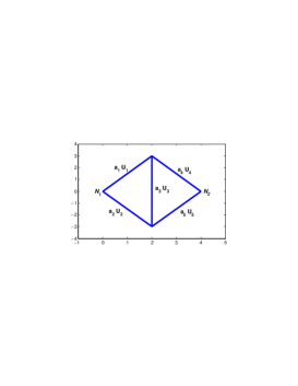
Fig. 1: A bridge network, in the case $d=5$

It is assumed that the lengths $\{U_{\ell},\ell\leq d\}$ are i.i.d. and uniformly distributed on $\left[0,1\right]$. We are interested in computing a threshold $\theta_{\star}$ such that the probability $\phi(U_{1},\cdots,U_{d})$ exceeds $\theta_{\star}$ is $1-q$ in the case $q$ is close to one. In this example,

$$\mathsf{X}=\left[0,1\right]^{d},\qquad p(u_{1},\cdots,u_{d})=\prod_{\ell=1}^{d}\mathbbm{1}_{\{\left[0,1\right]\}}(u_{\ell}).$$

The importance sampling distribution $g_{\nu}$ is a product of Beta$(\nu_{\ell},1)$ distributions:

$$\mathcal{V}=\left(\mathbb{R}^{+}\setminus\{0\}\right)^{d},\qquad g_{\nu}(u_{1},\cdots,u_{d})=\prod_{\ell=1}^{d}\nu_{\ell}\left(u_{\ell}\right)^{\nu_{\ell}-1}\mathbbm{1}_{\{\left[0,1\right]\}}(u_{\ell}).$$

$g_{\nu}$ is from a canonical exponential family with $S(u_{1},\cdots,u_{d})=\left(\ln u_{\ell}\right)_{1\leq\ell\leq d}$ and $B(\nu_{1},\cdots,\nu_{d})=\sum_{\ell=1}^{d}\ln\left(\nu_{\ell}\right)$. Furthermore, for any $1\leq\ell\leq d$, $\left(\hat{\nu}(s_{1},\cdots,s_{d})\right)_{\ell}=\left(-s_{\ell}\right)^{-1}$.

In this example, $\Theta=\mathbb{R}\times\prod_{\ell=1}^{d}\left(-\infty,0\right)$. The assumptions E 1 are easily verified with $\alpha=1$ (details are omitted). For the MCMC samplers $\{Q_{\theta},\theta\in\mathbb{R}\}$, we use a Gibbs sampler: note that for any $\ell\in\{1,\cdots,d\}$ and any $\{u_{j},j\neq\ell\}$, $u_{\ell}\mapsto\phi(u_{1},\cdots,u_{d})$ is increasing. Hence, the conditional distribution of the $\ell$-th variable conditionally to the others when the joint distribution is proportional to $p(x)\mathbbm{1}_{\{\phi(x)\geq\theta\}}$ is a uniform distribution on $\left[(\theta-\phi(u^{\ast}))_{+},1\right]$ where $u^{\ast}=(u_{1},\cdots,u_{\ell-1},0,u_{\ell+1},\cdots,u_{d})$.

We illustrate the convergence of SACE for the bridge network displayed on Figure 1 in the case $[\mathsf{a}_{1},\cdots,\mathsf{a}_{d}]=[1,2,3,1,2]$. On Figure 2[left], we show a path of $\{\theta_{n},n\geq 0\}$ for different runs of the algorithm corresponding to the different quantiles $q$. On Figure 2[right], we show the path of the $d$ components of $\hat{\nu}(\sigma_{n})$ in the case $q=0.001$. Not surprisingly, the largest values of the parameters $\hat{\nu}(\sigma_{n})_{\ell}$ at convergence are reached with $\ell=1,4$; they correspond to the shortest range of path length ($a_{1}=a_{4}=1$).

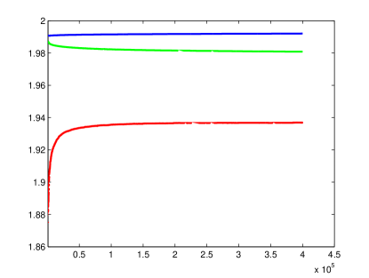
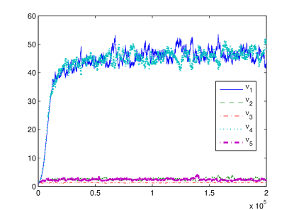
Fig. 2: [left] Paths of $\theta_{n}$ for different values of $q$ ($q=10^{-3},10^{-4}$ and $10^{-5}$) - the first $1000$ iterations are discarded. [Right] Path of the $d$ components of $\hat{\nu}(\sigma_{n})$, when $q=0.001$

3.3 Median in multi-dimensional spaces

In a multivariate setting different extensions of the median have been proposed in the literature (see for instance [11] and [12] and the references therein). We focus here on the spatial median, also named geometric median which is probably the most frequently used. The median $\theta$ of a random vector $X$ taking values in $\mathbb{R}^{d}$ with $d\geq 2$ is

$$\theta=\operatorname*{arg\,min}_{m\in\mathbb{R}^{d}}\mathbb{E}[\left|X-m\right|]$$

The median $\theta$ is uniquely defined unless the support of the distribution of $X$ is concentrated on a one dimensional subspace of $\mathbb{R}^{d}$. Note also that it is translation invariant. Following [11], we consider the stochastic approximation procedure with

$$H_{\theta}(x)\stackrel{{\scriptstyle\mathrm{def}}}{{=}}\frac{x-\theta}{\left|x-\theta\right|}\mathbbm{1}_{\{x\neq\theta\}},$$ (14)

and the following assumptions

E 2.

the condition H 2 is satisfied with $\pi_{\theta}=\pi$ for any $\theta$. The density $\pi$ is bounded on $\mathbb{R}^{d}$ and $\int\left|x\right|\pi(x)\mathrm{d}x<\infty$.

Proposition 3.4.

Assume E 2. Let $\theta_{\star}$ be the unique solution of $\int H_{\theta}(x)\pi(x)\mathrm{d}x=0$. Then H 1, H 4 and H 5 are satisfied with $w$ and $\mathcal{L}$ given by

$$w(\theta)=\int\left|x-\theta\right|\pi(x)\mathrm{d}x,\qquad\mathcal{L}=\{\theta_{\star}\},$$

and with $\alpha=d/(1+d)$.

Proof.

The proof is postponed to Section 5.3.

Here again, $w(\mathcal{L})$ has an empty interior; and theorem:general provides sufficient conditions on the kernels $\{P_{\theta},\theta\in\Theta\}$ and on the sequence $\{\gamma_{n},n\geq 0\}$ implying that $\{\theta_{n},n\geq 0\}$ converges almost-surely to $\theta_{\star}$.

3.4 Vector quantization

Vector quantization consists of approximating a random vector $X$ in $\mathbb{R}^{d}$ by a random vector taking at most $N$ values in $\mathbb{R}^{d}$. In this section, we assume that

E 3.

the distribution of $X$ is absolutely continuous with respect to the Lebesgue measure on $\mathbb{R}^{d}$ with density $\pi$ having a bounded support: $\pi(x)=0$ for any $\left|x\right|>\Delta$ for some $\Delta>0$.

Vector quantization plays a crucial role in source coding [38], numerical integration [31, 33] and nonlinear filtering [32, 34]. Several stochastic approximations procedure have been proposed to approximate the optimal quantizer; see [20, 8]. For ${\bf\theta}=(\theta^{(1)},\theta^{(2)},\dots,\theta^{(N)})\in(\mathbb{R}^{d})^{N}$, and for any $1\leq i\leq N$, define the Voronoi cells associated to the dictionary $\theta$ by

$${C}^{(i)}({\bf\theta})\stackrel{{\scriptstyle\mathrm{def}}}{{=}}\left\{u\in\mathbb{R}^{d},\left|u-\theta^{(i)}\right|=\min\limits_{1\leq j\leq N}\left|u-\theta^{(j)}\right|\right\}.$$

These cells allow to approximate a random vector $X$ by $\theta^{(i)}$ in the cell $C^{(i)}({\bf\theta})$. Denote by $\widetilde{w}$ the mean squared quantization error (or distortion) given by

$$\widetilde{w}({\bf\theta})\stackrel{{\scriptstyle\mathrm{def}}}{{=}}\sum_{i=1}^{N}\mathbb{E}_{\pi}\left[\left|X-\theta^{(i)}\right|^{2}\mathbbm{1}_{\{C^{(i)}({\bf\theta})\}}(X)\right].$$

The Kohonen algorithm (with 0 neighbors) is a stochastic approximation algorithm with field $\widetilde{H}:(\mathbb{R}^{d})^{N}\times\mathbb{R}^{d}\to(\mathbb{R}^{d})^{N}$ given by

$$\widetilde{H_{{\bf\theta}}}(u)\stackrel{{\scriptstyle\mathrm{def}}}{{=}}-2\left((\theta^{(i)}-u)\mathbbm{1}_{\{C^{(i)}({\bf\theta})\}}(u)\right)_{1\leq i\leq N}.$$

The convergence of the Kohonen algorithm has been established in dimension $d=1$ for i.i.d. observations $\{X_{n},n\in\mathbb{N}\}$ [31]. The case $d\geq 2$ is still an open question: one of the main difficulty arises from the non-coercivity of the distortion $\widetilde{w}$ and the non-smoothness property of the field $\widetilde{H_{\theta}}(x)$. The goal here is to go a step further in the study of the multidimensional case, including a generalization to the case the observations $\{X_{k},k\geq 1\}$ are Markovian (see e.g. [33, 34]):

E 4.

$\{P_{{\bf\theta}},{\bf\theta}\in\Theta\}$ is a family of kernels satisfying H 2 for some $p\geq 2$, H 3 and such that $\pi_{{\bf\theta}}=\pi$ for any ${\bf\theta}\in\Theta$.

We define

$$\Theta=\left\{{\bf\theta}=(\theta^{(1)},\dots\theta^{(N)})\in(\mathbb{R}^{d})^{N}\cap(\mathcal{B}(0,\Delta))^{N},\theta^{(i)}\neq\theta^{(j)}\ \text{for all $i\neq j$}\right\};$$

and run Algorithm 2 with $H_{{\bf\theta}}\in\mathbb{R}^{dN}$ defined by

$$H_{{\bf\theta}}(x)=\widetilde{H_{{\bf\theta}}}(x)-\lambda\left(\sum_{j\neq i}\frac{\theta^{(i)}-\theta^{(j)}}{\left|\theta^{(i)}-\theta^{(j)}\right|^{4}}\right)_{1\leq i\leq N}$$ (15)

for some $\lambda>0$ with the sequence of compact sets $\mathcal{K}_{q}=\{{\bf\theta}\in\Theta:\min_{i\neq j}\left|\theta^{(i)}-\theta^{(j)}\right|\geq 1/q\}$. Set

$$w({\bf\theta})=\widetilde{w}({\bf\theta})+\frac{\lambda}{4}\sum_{i\neq j}\left|\theta^{(i)}-\theta^{(j)}\right|^{-2}.$$ (16)

Under E 3, from [31, Proposition 9 and Lemma 29], $w$ is continuously differentiable on $\Theta$ and $\nabla w({\bf\theta})=-\int H_{{\bf\theta}}(x)\pi(x)\,\mathrm{d}x$. Furthermore, for any compact set $\mathcal{K}_{q}$, there exists a constant $C$ such that for any ${\bf\theta}\in\mathcal{K}_{q}$, $\bar{\bf\theta}\in\mathcal{K}_{q}$, $\left|\nabla w(\theta)-\nabla w(\bar{\bf\theta})\right|\leq C\left|{\bf\theta}-\bar{\bf\theta}\right|$. Hence, $\nabla w$ is locally Lipschitz on $\Theta$.

Lemma 3.5.

Assume E 3 and E 4. Then H 1, H 4 and H 5 are satisfied with $w$ defined by (16) and $\mathcal{L}\stackrel{{\scriptstyle\mathrm{def}}}{{=}}\{\theta\in\Theta:\nabla w(\theta)=0\}$.

Proof.

The proof is postponed in Section 5.4.

Theorem 2.1 shows that under E 3, E 4, the penalized $0$-neighbors Kohonen algorithm converges a.s. to a connected component of $\mathcal{L}$.

4 Proofs

In Section 4.1, we start with preliminary results on the stability and the convergence of stochastic approximation schemes. We provide a new set of sufficient conditions for the convergence of stable SA algorithms (see Proposition 4.11). In Section 4.2, some properties of the Poisson equations associated to the transition kernels $\{P_{\theta},\theta\in\Theta\}$ are discussed. In Section 4.3, we first state a control of the perturbations $H_{\theta_{n}}(X_{n+1})-h(\theta_{n})$ (see Proposition 4.16) which is the key ingredient for the proof of Theorem 2.1; we then conclude Section 4.3 by giving the proof of Theorem 2.1. The proof of Proposition 4.16 is given in Section 4.4.

4.1 Stability and Convergence of Stochastic Approximation algorithms

Let $\{\vartheta_{n},n\geq 0\}$ be defined, for all $\vartheta_{0}\in\Theta$ and $n\geq 1$ by:

$$\vartheta_{n}=\vartheta_{n-1}+\rho_{n}h(\vartheta_{n-1})+\rho_{n}\xi_{n},$$ (17)

where $\{\rho_{n},n\in\mathbb{N}\}$ is a sequence of positive numbers and $\{\xi_{n},n\in\mathbb{N}\}$ is a sequence of $\mathbb{R}^{d}$-vectors. For any $L\geq 0$, the sequence $\{\tilde{\vartheta}_{L,k},k\geq 0\}$ is defined by $\tilde{\vartheta}_{L,0}=\vartheta_{L}$, and for $k\geq 1$,

$$\tilde{\vartheta}_{L,k}=\tilde{\vartheta}_{L,k-1}+\rho_{L+k}h(\vartheta_{L+k-1}).$$ (18)

Lemma 4.6.

Assume H 5. Let $M_{0}$ be such that $\{\vartheta_{0}\}\cup\mathcal{L}\subset\{\vartheta:w(\vartheta)\leq M_{0}\}$. There exist $\delta_{\star}>0$ and $\lambda_{\star}>0$ such that for any non-increasing sequence $\{\rho_{n},n\in\mathbb{N}\}$ of positive numbers and any $\mathbb{R}^{d}$-valued sequence $\{\xi_{n},n\in\mathbb{N}\}$

$$\left(\rho_{0}\leq\lambda_{\star}\ \text{and}\ \sup_{k\geq 1}\left|\sum_{j=1}^{k}\rho_{j}\xi_{j}\right|\leq\delta_{\star}\right)\Longrightarrow\left(\sup_{k\geq 1}w(\vartheta_{k})\leq M_{0}+1\right).$$

Proof.

See [3, Theorem 2.2].

Lemma 4.7.

Let $g:\Theta\to\mathbb{R}$ be a continuous function. For any compact set $\mathcal{K}\subset\Theta$ and $\delta>0$, there exists $\eta>0$ such that for all $\vartheta\in\mathcal{K}$ and $\vartheta^{\prime}\in\Theta$ satisfying $|\vartheta-\vartheta^{\prime}|\leq\eta$, $|g(\vartheta)-g(\vartheta^{\prime})|\leq\delta$.

Lemma 4.8.

Assume H 5-(c) and $h$ is continuous. For any compact set $\mathcal{K}$ of $\Theta$ such that $\mathcal{K}\cap\mathcal{L}=\emptyset$ and any $\delta\in\left(0,\inf_{\mathcal{K}}|\left<\nabla w,h\right>|\right)$, there exist $\lambda>0,\beta>0$ such that for all $\vartheta\in\mathcal{K}$, $\rho\leq\lambda$ and $|\xi|\leq\beta$, $w\left(\vartheta+\rho h(\vartheta)+\rho\xi\right)\leq w(\vartheta)-\rho\delta$.

Proof.

See [3, Lemma 2.1(i)].

Lemma 4.9.

Assume H 5, $h$ is continuous, $\lim_{n}\rho_{n}=0$, $\lim_{k}\sum_{j=1}^{k}\rho_{j}\xi_{j}$ exists and there exists $M>0$ such that for any $n\geq 0$, $\vartheta_{n}\in\mathcal{K}\stackrel{{\scriptstyle\mathrm{def}}}{{=}}\{\theta\in\Theta:w(\theta)\leq M\}$. Then

1. for any $L\geq 0$ and $k\geq 0$, $\vartheta_{L+k+1}-\tilde{\vartheta}_{L,k+1}=\sum_{j=L}^{L+k}\rho_{j+1}\xi_{j+1}$.

2. $\limsup_{n\to\infty}|\vartheta_{n+1}-\vartheta_{n}|=0$.

3. for any $\widetilde{M}>M$, there exists $\tilde{L}$ such that for any $L\geq\tilde{L}$, $\{\tilde{\vartheta}_{L,k},k\geq 0\}\subset\widetilde{\mathcal{K}}\stackrel{{\scriptstyle\mathrm{def}}}{{=}}\{\theta\in\Theta:w(\theta)\leq\widetilde{M}\}$.

4. $\lim_{L\to\infty}\sup_{l\geq 0}|w(\tilde{\vartheta}_{L,l})-w(\vartheta_{L+l})|=0$.

Proof.

1. (18) implies that $\tilde{\vartheta}_{L,k+1}-\vartheta_{L+k+1}=\tilde{\vartheta}_{L,k}-\vartheta_{L+k}-\rho_{L+k+1}\xi_{L+k+1}$ from which the proof follows.

2. Under H 5-(a) and the continuity of $h$ on $\Theta$, $\sup_{\mathcal{K}}|h|<+\infty$. Since $\vartheta_{k}\in\mathcal{K}$ for any $k$, we get $|\tilde{\vartheta}_{L,k+1}-\tilde{\vartheta}_{L,k}|\leq\rho_{L+k+1}\sup_{\mathcal{K}}|h|$. Let $\epsilon>0$. Under the stated assumptions, we may choose $K_{\epsilon}$ such that for any $k\geq K_{\epsilon}$ and $L\geq 0$, $|\tilde{\vartheta}_{L,k}-\tilde{\vartheta}_{L,k-1}|\leq\epsilon$ and $L_{\epsilon}$ such that for any $L\geq L_{\epsilon}$, $\sup_{l\geq 1}|\sum_{j=L}^{L+l}\rho_{j+1}\xi_{j+1}\mathbbm{1}_{\vartheta_{j}\in\mathcal{K}}|\leq\epsilon$. By (i), for any $k\geq K_{\epsilon}$ and $L=L_{\epsilon}$,

   $$\left|\vartheta_{L+k+1}-\vartheta_{L+k}\right|\leq\left|\tilde{\vartheta}_{L,k+1}-\tilde{\vartheta}_{L,k}\right|+\left|\vartheta_{L+k+1}-\tilde{\vartheta}_{L,k+1}\right|+\left|\tilde{\vartheta}_{L,k}-\vartheta_{L+k}\right|\leq 3\epsilon.$$

3. $\widetilde{\mathcal{K}}$ is compact by H 5-(a). By Lemma 4.7, there exists $\eta>0$ such that for all $\vartheta\in\mathcal{K}$, $\vartheta^{\prime}\in\Theta$, $|\vartheta-\vartheta^{\prime}|\leq\eta$, $\left|w(\vartheta)-w(\vartheta^{\prime})\right|\leq\widetilde{M}-M$. There exists $\tilde{L}$ such that for any $L\geq\tilde{L}$, $\sup_{l\geq 1}|\sum_{j=L}^{L+l}\rho_{j+1}\xi_{j+1}\mathbbm{1}_{\vartheta_{j}\in\mathcal{K}}|\leq\eta$. By (i), $\sup_{L\geq\tilde{L}}\sup_{k\geq 0}|\tilde{\vartheta}_{L,k}-\vartheta_{L+k}|\leq\eta$. Since $\vartheta_{j}\in\mathcal{K}$ for any $j\geq 0$, this implies that for any $L\geq\tilde{L}$ and $k\geq 0$, $w(\tilde{\vartheta}_{L,k})\leq\widetilde{M}$ and $\tilde{\vartheta}_{L,k}\in\widetilde{\mathcal{K}}$.

4. The proof is on the same lines as the proof of (iii).

Lemma 4.10.

Let $\{v_{n},n\geq 0\}$ and $\{\chi_{n},n\geq 0\}$ be non-negative sequences and $\{\eta_{n},n\geq 0\}$ be a sequence such that $\sum_{n}\eta_{n}$ exists. If for any $n\geq 0$, $v_{n+1}\leq v_{n}-\chi_{n}+\eta_{n}$ then $\sum_{n}\chi_{n}<\infty$ and $\lim_{n}v_{n}$ exists.

Proof.

Set $w_{n}=v_{n}+\sum_{k\geq n}\eta_{k}+M$ with $M\stackrel{{\scriptstyle\mathrm{def}}}{{=}}-\inf_{n}\sum_{k\geq n}\eta_{k}$ so that $\inf_{n}w_{n}\geq 0$. Then

$$0\leq w_{n+1}\leq v_{n}-\chi_{n}+\eta_{n}+\sum_{k\geq n+1}\eta_{k}+M\leq w_{n}-\chi_{n}.$$

Hence, the sequence $\{w_{n},n\geq 0\}$ is non-negative and non-increasing; therefore it converges. Furthermore, $0\leq\sum_{k=0}^{n}\chi_{k}\leq w_{0}$ so that $\sum_{n}\chi_{n}<\infty$. Therefore, the convergence of $\{w_{n},n\geq 0\}$ also implies the convergence of $\{v_{n},n\geq 0\}$. This concludes the proof.

Proposition 4.11.

Assume H 5. Let $\{\rho_{n},n\in\mathbb{N}\}$ be a non-increasing sequence of positive numbers and $\{\xi_{n},n\in\mathbb{N}\}$ be a sequence of $\mathbb{R}^{d}$-vectors. Assume

1. $h:\Theta\to\mathbb{R}^{d}$ is continuous.

2. $\{\vartheta_{k},k\in\mathbb{N}\}\subset\mathcal{K}\stackrel{{\scriptstyle\mathrm{def}}}{{=}}\{\theta\in\Theta:w(\theta)\leq M\}$.

3. $\sum_{k}\rho_{k}=+\infty$ and $\lim_{k}\rho_{k}=0$.

4. $\lim_{k\to\infty}\sum_{j=1}^{k}\rho_{j}\xi_{j}$ exists.

5. one of the following conditions

   1. $w(\mathcal{L})$ has an empty interior

   2. $\nabla w$ is locally Lipschitz on $\Theta$, and the series $\sum\rho_{j}\left<\nabla w(\vartheta_{j}),\xi_{j}\right>$ and $\sum_{j}\rho_{j}^{2}\left|\xi_{j}\right|^{2}$ converge.

Then $\{\vartheta_{n},n\geq 0\}$ converges to a connected component of $\mathcal{L}$.

Proof.

Assume first that $\lim_{n\to\infty}w(\vartheta_{n})$ exists.

$\blacktriangleright$ Step 1. For $\alpha>0$, let $\mathcal{L}_{\alpha}\stackrel{{\scriptstyle\mathrm{def}}}{{=}}\{\theta\in\Theta:\mathrm{d}(\theta,\mathcal{L})<\alpha\}$ be the $\alpha$-neighborhood of $\mathcal{L}$. Let $\epsilon>0$. We prove that there exist $L_{\epsilon}$ and $\delta_{1}>0$ such that for any $L\geq L_{\epsilon}$,

1. $\sup_{k\geq 0}\left|\tilde{\vartheta}_{L,k}-\vartheta_{L+k}\right|\leq\epsilon$ and $\sup_{k\geq 0}\left|w(\tilde{\vartheta}_{L,k})-w(\vartheta_{L+k})\right|\leq\epsilon$.

2. for any $k\geq 0$, it holds: $\tilde{\vartheta}_{L,k}\notin\mathcal{L}_{\alpha}\Longrightarrow w(\tilde{\vartheta}_{L,k+1})-w(\tilde{\vartheta}_{L,k})\leq-\rho_{L+k+1}\delta_{1}$.

3. the sequence $\{\tilde{\vartheta}_{L,k},k\geq 0\}$ is infinitely often in $\mathcal{L}_{\alpha}$.

Let $\widetilde{M}>M$ and set $\widetilde{\mathcal{K}}\stackrel{{\scriptstyle\mathrm{def}}}{{=}}\{\theta\in\Theta:w(\theta)\leq\widetilde{M}\}$. Note that by H 5-(a), $\widetilde{\mathcal{K}}\subset\Theta$ is compact and since $\mathcal{L}_{\alpha}$ is open, $\widetilde{\mathcal{K}}^{\alpha}\stackrel{{\scriptstyle\mathrm{def}}}{{=}}\widetilde{\mathcal{K}}\setminus\mathcal{L}_{\alpha}$ is compact and $\widetilde{\mathcal{K}}^{\alpha}\cap\mathcal{L}=\emptyset$. By Lemma 4.8, there exist $\delta_{1}>0$, $\lambda_{1}>0$, $\beta_{1}>0$ such that

$$\left(\vartheta\in\widetilde{\mathcal{K}}^{\alpha},\rho\leq\lambda_{1},|\xi|\leq\beta_{1}\right)\Longrightarrow w\left(\vartheta+\rho h(\vartheta)+\rho\xi\right)\leq w(\vartheta)-\rho\delta_{1}.$$ (19)

By Lemma 4.7, there exists $\delta_{2}\in\left(0,\epsilon\right)$ such that

$$\left(\vartheta\in\mathcal{K},\vartheta^{\prime}\in\Theta,|\vartheta-\vartheta^{\prime}|\leq\delta_{2}\right)\Longrightarrow\left(\left|h(\vartheta)-h(\vartheta^{\prime})\right|\leq\beta_{1},\ \ \left|w(\vartheta)-w(\vartheta^{\prime})\right|\leq\epsilon\right).$$ (20)

By Lemma 4.9-(iii), (C-iii) and (C-iv), there exists $\widetilde{L}$ such that for any $L\geq\widetilde{L}$, $\{\tilde{\vartheta}_{L,k},k\geq 0\}\subset\widetilde{\mathcal{K}}$ and

$$\sup_{k\geq 0}\rho_{L+k}\leq\lambda_{1},\qquad\sup_{l\geq 1}\left|\sum_{j=L}^{L+l}\rho_{j+1}\xi_{j+1}\mathbbm{1}_{\vartheta_{j}\in\mathcal{K}}\right|\leq\delta_{2}.$$ (21)

1. follows from Lemma 4.9-(i) and (21).

2. Let $L\geq\tilde{L}$, $k\geq 0$ and $\tilde{\vartheta}_{L,k}\not\in\mathcal{L}_{\alpha}$. The proof follows from (19) and

   $$\tilde{\vartheta}_{L,k+1}=\tilde{\vartheta}_{L,k}+\rho_{L+k+1}h\left(\tilde{\vartheta}_{L,k}\right)+\rho_{L+k+1}\left(h\left(\vartheta_{L+k}\right)-h\left(\tilde{\vartheta}_{L,k}\right)\right),$$

   using (20) and (21).

3. The proof is by contradiction. Let $L\geq\widetilde{L}$, $k\geq 0$ and assume that for any $j\geq 0$, $\tilde{\vartheta}_{L,k+j}\in\widetilde{\mathcal{K}}^{\alpha}$. By (b), for any $j,k\geq 0$, $w\left(\tilde{\vartheta}_{L,k+j+1}\right)\leq w(\tilde{\vartheta}_{L,k+j})-\rho_{L+k+j+1}\delta_{1}$ which implies under (C-iii) that $\lim_{j\to\infty}w(\tilde{\vartheta}_{L,k+j})=-\infty$. Since $w$ is continuous and nonnegative and $\mathcal{K}$ compact, $\inf_{\widetilde{\mathcal{K}}}w\geq 0$. This is a contradiction.

$\blacktriangleright$ Step 2. Let $\alpha>0$ and $\epsilon>0$. By Step 1 and Lemma 4.9-(iv), there exists $L_{\epsilon}$ such that for any $L\geq L_{\epsilon}$ and $k\geq 0$, $\sigma_{L,k}\stackrel{{\scriptstyle\mathrm{def}}}{{=}}\inf\{j\geq 0,\tilde{\vartheta}_{L,k+j}\in\mathcal{L}_{\alpha}\}$ is finite, $\sup_{k\geq 0}\left|\tilde{\vartheta}_{L,k}-\vartheta_{L+k}\right|\leq\epsilon$, $\sup_{k\geq 0}\left|w(\tilde{\vartheta}_{L,k})-w(\vartheta_{L+k})\right|\leq\epsilon$ and

$$\delta_{1}\sum_{\ell=1}^{\sigma_{L,k}}\rho_{L+k+\ell}\leq w(\tilde{\vartheta}_{L,k})-w(\tilde{\vartheta}_{L,k+\sigma_{L,k}}).$$

Hence, for any $k\geq 0$, using $|\tilde{\vartheta}_{L,\ell}-\tilde{\vartheta}_{L,\ell-1}|\leq\rho_{L+\ell}\sup_{\mathcal{K}}|h|$,

$$\mathrm{d}\left(\vartheta_{L+k},\mathcal{L}_{\alpha}\right) \leq\left|\vartheta_{L+k}-\tilde{\vartheta}_{L,k+\sigma_{L,k}}\right|\leq\left|\vartheta_{L+k}-\tilde{\vartheta}_{L,k}\right|+\left|\tilde{\vartheta}_{L,k}-\tilde{\vartheta}_{L,k+\sigma_{L,k}}\right|$$

$$\leq\epsilon+\sum_{\ell=1}^{\sigma_{L,k}}\left|\tilde{\vartheta}_{L,k+\ell}-\tilde{\vartheta}_{L,k+\ell-1}\right|\leq\epsilon+\sup_{\mathcal{K}}|h|\,\sum_{\ell=1}^{\sigma_{L,k}}\rho_{L+k+\ell}$$

$$\leq\epsilon+\delta_{1}^{-1}\sup_{\mathcal{K}}|h|\,\sup_{\ell\geq 0}\left|w(\tilde{\vartheta}_{L,k})-w(\tilde{\vartheta}_{L,k+\ell})\right|,$$

$$\leq\epsilon+2\epsilon\delta_{1}^{-1}\sup_{\mathcal{K}}|h|+\delta_{1}^{-1}\sup_{\mathcal{K}}|h|\,\sup_{\ell\geq 0}\left|w(\vartheta_{L+k})-w(\vartheta_{L+k+\ell})\right|.$$

This proves that $\lim_{n}\mathrm{d}(\vartheta_{n},\mathcal{L})=0$ since $\lim_{n}w(\vartheta_{n})$ exists. Finally, since by Lemma 4.9-(ii), $\lim_{n}|\vartheta_{n}-\vartheta_{n-1}|=0$, the sequence $\{\vartheta_{n},n\geq 0\}$ converges to a connected component of $\mathcal{L}$.

$\blacktriangleright$ Step 3. We now prove that $\lim_{n}w(\vartheta_{n})$ exists. Under (C-v)-(C-v)(A), the proof follows from [3, Theorem 2.3]. We prove that this limit exists under (C-v)-(C-v)(B).

By H 5-(a), (C-ii) and Lemma 4.9-(ii), there exist $N$ and a compact set $\widetilde{\mathcal{K}}$ of $\Theta$ such that $\mathcal{K}\subseteq\widetilde{\mathcal{K}}$ and for any $n\geq N$ and $t\in\left[0,1\right]$, $\vartheta_{n}+t(\vartheta_{n+1}-\vartheta_{n})\in\widetilde{\mathcal{K}}$. By (C-v)-(C-v)(B), there exists a constant $C$ such that for $\vartheta,\vartheta^{\prime}\in\widetilde{\mathcal{K}}$, $|\nabla w(\vartheta)-\nabla w(\vartheta^{\prime})|\leq C|\vartheta-\vartheta^{\prime}|$ showing that, for $n\geq N$,

$$w(\vartheta_{n+1}) \leq w(\vartheta_{n})+\left<\nabla w(\vartheta_{n}),\vartheta_{n+1}-\vartheta_{n}\right>+C/2\left|\vartheta_{n+1}-\vartheta_{n}\right|^{2}.$$

Using (17), we obtain

$$\left<\nabla w(\vartheta_{n}),\vartheta_{n+1}-\vartheta_{n}\right>=\rho_{n+1}\left<\nabla w(\vartheta_{n}),h(\vartheta_{n})\right>+\rho_{n+1}\left<\nabla w(\vartheta_{n}),\xi_{n+1}\right>$$

$$|\vartheta_{n+1}-\vartheta_{n}|^{2}\leq 2\rho^{2}_{n+1}\left\{\left(\sup_{\mathcal{K}}|h|\right)^{2}+|\xi_{n+1}|^{2}\right\}.$$

This yields for any $n\geq N$,

$$w(\vartheta_{n+1})\leq w(\vartheta_{n})-\rho_{n+1}\left|\left<\nabla w(\vartheta_{n}),h(\vartheta_{n})\right>\right|+\rho_{n+1}\left<\nabla w(\vartheta_{n}),\xi_{n+1}\right>\\ +C\,\rho_{n+1}^{2}\left(\left(\sup_{\mathcal{K}}|h|\right)^{2}+|\xi_{n+1}|^{2}\right).$$

Lemma 4.10 concludes the proof.

4.2 Regularity in $\theta$ of the solution to the Poisson equation

Under the assumptions H 1 and H 2, for any $\theta\in\Theta$, there exists a function $g$ solving the Poisson equation

$$g\mapsto H_{\theta}-\pi_{\theta}H_{\theta}=g-P_{\theta}g.$$ (22)

This solution, denoted by $g_{\theta}$, is unique up to an additive constant and given by $g_{\theta}(x)\stackrel{{\scriptstyle\mathrm{def}}}{{=}}\sum_{n\geq 0}\left\{P_{\theta}^{n}H_{\theta}(x)-\pi_{\theta}H_{\theta}\right\}$. Finally, for any compact set $\mathcal{K}$ of $\Theta$,

$$\sup_{\theta\in\mathcal{K}}\left|g_{\theta}\right|_{W}\leq\sup_{\theta\in\mathcal{K}}|H_{\theta}|_{W}\ \sum_{n\geq 0}\sup_{x\in\mathsf{X}}\frac{\sup_{\theta\in\mathcal{K}}\|P_{\theta}^{n}(x,\cdot)-\pi_{\theta}\|_{W}}{W(x)}\,<\infty.$$ (23)

Lemma 4.12.

Assume H 2-(b). For any compact set $\mathcal{K}\subset\Theta$, there exists a constant $C$ such that for any $\theta,\theta^{\prime}\in\mathcal{K}$

$$\sup_{n\geq 0}\sup_{x\in\mathsf{X}}\frac{\|P_{\theta}^{n}(x,.)-P_{\theta^{\prime}}^{n}(x,.)\|_{W}}{W(x)}\leq CD_{W}(\theta,\theta^{\prime}),$$

where $D_{W}$ is defined by (3).

Proof.

For any measurable function $f$ such that $|f|_{W}\leq 1$, it holds

$$P_{\theta}^{n}f(x)-P_{\theta^{\prime}}^{n}f(x) =\sum_{j=0}^{n-1}P_{\theta^{\prime}}^{j}(P_{\theta}-P_{\theta^{\prime}})\left(P_{\theta}^{n-j-1}f(x)-\pi_{\theta}(f)\right).$$

For any $0\leq j\leq n-1$,

$$\left|P_{\theta^{\prime}}^{j}(P_{\theta}-P_{\theta^{\prime}})\left(P_{\theta}^{n-j-1}f(x)-\pi_{\theta}(f)\right)\right| \leq P_{\theta^{\prime}}^{j}W(x)\left|(P_{\theta}-P_{\theta^{\prime}})\left(P_{\theta}^{n-j-1}f-\pi_{\theta}(f)\right)\right|_{W}$$

$$\leq D_{W}(\theta,\theta^{\prime})\ P_{\theta^{\prime}}^{j}W(x)\left|P_{\theta}^{n-j-1}f-\pi_{\theta}(f)\right|_{W}.$$

By H 2-(b), there exist $C>0$ and $\lambda\in\left(0,1\right)$ such that for any $\theta,\theta^{\prime}\in\mathcal{K}$,

$$P_{\theta^{\prime}}^{j}W(x)\left|P_{\theta}^{n-j-1}f-\pi_{\theta}(f)\right|_{W}\leq C\left(\lambda^{j}W(x)+\pi_{\theta^{\prime}}(W)\right)\lambda^{n-j-1}.$$

This concludes the proof.

Lemma 4.13.

Assume H 2-(a),(b). For any compact set $\mathcal{K}\subset\Theta$, there exists $C>0$ such that for any $\theta,\theta^{\prime}\in\mathcal{K}$, $\|\pi_{\theta}-\pi_{\theta^{\prime}}\|_{W}\leq CD_{W}(\theta,\theta^{\prime})$.

Proof.

For any $x\in\mathsf{X},n\in\mathbb{N}$,

$$\|\pi_{\theta}-\pi_{\theta^{\prime}}\|_{W} \leq\left\|\pi_{\theta}-P_{\theta}^{n}(x,\cdot)\right\|_{W}+\left\|P_{\theta}^{n}(x,\cdot)-P_{\theta^{\prime}}^{n}(x,\cdot)\right\|_{W}+\left\|P_{\theta^{\prime}}^{n}(x,\cdot)-\pi_{\theta^{\prime}}\right\|_{W}.$$

Let $\mathcal{K}$ be a compact subset of $\Theta$. By H 2-(b), there exist constants $C>0$ and $\lambda\in\left(0,1\right)$ such that for any $n\in\mathbb{N}$ and $x\in\mathsf{X}$ $\sup_{\theta\in\mathcal{K}}\left\|\pi_{\theta}-P_{\theta}^{n}(x,\cdot)\right\|_{W}\leq C\lambda^{n}W(x)$. Moreover, using Lemma 4.12, there exists a constant $C^{\prime}>0$ such that for any $\theta,\theta^{\prime}\in\mathcal{K}$ and any $x\in\mathsf{X}$, $\sup_{n\geq 0}\left\|P_{\theta}^{n}(x,\cdot)-P_{\theta^{\prime}}^{n}(x,\cdot)\right\|_{W}\leq C^{\prime}D_{W}(\theta,\theta^{\prime})W(x)$. The proof follows, upon noting that $x$ is fixed and arbitrarily chosen.

Lemma 4.14.

Assume H 1, H 2-(a),(b) and H 4. For any compact set $\mathcal{K}\subset\Theta$, there exists $C>0$ such that for any $\theta,\theta^{\prime}\in\mathcal{K}$,

$$\left|h(\theta)-h(\theta^{\prime})\right|\leq C\left(D_{W}(\theta,\theta^{\prime})+\left|\theta-\theta^{\prime}\right|^{\alpha}\right),$$

where $D_{W}$ and $\alpha$ are given by (3) and H 4.

Proof.

Let $\mathcal{K}$ be a compact subset of $\Theta$ and $\theta$, $\theta^{\prime}$ in $\mathcal{K}$. By definition of $h$, it holds

$$\left|h(\theta)-h(\theta^{\prime})\right| =\left|\pi_{\theta}H_{\theta}-\pi_{\theta^{\prime}}H_{\theta^{\prime}}\right|\leq\pi_{\theta}\left|H_{\theta}-H_{\theta^{\prime}}\right|+\left|(\pi_{\theta}-\pi_{\theta^{\prime}})H_{\theta^{\prime}}\right|.$$

Condition H 4 implies that there exists a constant $C>0$ such that for any $\theta,\theta^{\prime}\in\mathcal{K}$, $\pi_{\theta}\left|H_{\theta}-H_{\theta^{\prime}}\right|\leq C\left|\theta-\theta^{\prime}\right|^{\alpha}$. By Lemma 4.13 and H 1, there exist $C>0$ such that for any $\theta,\theta^{\prime}\in\mathcal{K}$, $\left|(\pi_{\theta}-\pi_{\theta^{\prime}})H_{\theta^{\prime}}\right|\leq CD_{W}(\theta,\theta^{\prime})$. The proof follows.

For any $\vartheta\in\Theta$, $x\in\mathsf{X}$ and $L\geq 0$, set

$$\mathcal{H}_{\vartheta,L}(x)\stackrel{{\scriptstyle\mathrm{def}}}{{=}}\sup_{\{\theta\in\mathcal{K}:\|\theta-\vartheta\|\leq L\}}\left|H_{\theta}(x)-H_{\vartheta}(x)\right|.$$ (24)

Proposition 4.15.

Assume H 1, H 2-(a),(b), and H 4. Let $g_{\theta}$ be the solution of (22). For any compact set $\mathcal{K}\subset\Theta$, there exist constants $C>0$ and $\lambda\in\left(0,1\right)$ such that for any $\theta,\theta^{\prime}\in\mathcal{K}$, $x\in\mathsf{X}$, $n\geq 1$, $L>0$, and any $\vartheta\in\mathcal{K}$ such that $\left|\theta-\vartheta\right|\leq L$,

$$\left|P_{\theta}g_{\theta}(x)-P_{\theta^{\prime}}g_{\theta^{\prime}}(x)\right|\leq C\Big{\{}\lambda^{n}W(x)+2\,\sum_{l=1}^{n}P_{\vartheta}^{l}\mathcal{H}_{\vartheta,L}(x)\\ +n\,\left|\theta-\theta^{\prime}\right|^{\alpha}+n\,D_{W}(\theta,\theta^{\prime})+n\,D_{W}(\theta,\vartheta)W(x)+n\,D_{W}(\theta^{\prime},\vartheta)W(x)\Big{\}}.$$

Proof.

For any $\theta,\theta^{\prime}\in\Theta$ and any $n\geq 1$, we write

$$P_{\theta}g_{\theta}(x)-P_{\theta^{\prime}}g_{\theta^{\prime}}(x) =\sum_{l>n}\{P_{\theta}^{l}H_{\theta}(x)-h(\theta)\}-\sum_{l>n}\{P_{\theta^{\prime}}^{l}H_{\theta^{\prime}}(x)-h(\theta^{\prime})\}+\psi\left(h(\theta^{\prime})-h(\theta)\right)$$

$$+\sum_{l=1}^{n}\{P_{\theta}^{l}H_{\theta}(x)-P_{\theta^{\prime}}^{l}H_{\theta^{\prime}}(x)\}.$$

We first prove that

$$\left|P_{\theta}g_{\theta}(x)-P_{\theta^{\prime}}g_{\theta^{\prime}}(x)-\sum_{l=1}^{n}\{P_{\theta}^{l}H_{\theta}(x)-P_{\theta^{\prime}}^{l}H_{\theta^{\prime}}(x)\}\right|\\ \leq C\left(\lambda^{n}W(x)+n\,D_{W}(\theta,\theta^{\prime})+n\,\left|\theta-\theta^{\prime}\right|^{\alpha}\right).$$ (25)

By H 1 and H 2-(b), for any compact set $\cal K$, there exist constants $C>0$ and $\lambda\in\left(0,1\right)$ such that for any $x,n$

$$\sup_{\theta\in\mathcal{K}}\left|\sum_{l>n}\{P_{\theta}^{l}H_{\theta}(x)-h(\theta)\}\right|\leq C\lambda^{n+1}\sup_{\theta\in\mathcal{K}}|H_{\theta}|_{W}\,W(x).$$

(25) follows from this inequality and Lemma 4.14. We now establish an upper bound for $\left|\sum_{l=1}^{n}\{P_{\theta}^{l}H_{\theta}(x)-P_{\theta^{\prime}}^{l}H_{\theta^{\prime}}(x)\}\right|$; we first write

$$\sum_{l=1}^{n}\left|P_{\theta}^{l}H_{\theta}(x)-P_{\theta^{\prime}}^{l}H_{\theta^{\prime}}(x)\right|\leq\sum_{l=1}^{n}\left|P_{\theta}^{l}H_{\theta}(x)-P_{\vartheta}^{l}H_{\vartheta}(x)\right|+\sum_{l=1}^{n}\left|P_{\vartheta}^{l}H_{\vartheta}(x)-P_{\theta^{\prime}}^{l}H_{\theta^{\prime}}(x)\right|.$$

For any $l\geq 1$ and $\vartheta\in\mathcal{K}$ such that $\left|\theta-\vartheta\right|\leq L$, we have

$$\left|P_{\theta}^{l}H_{\theta}(x)-P_{\vartheta}^{l}H_{\vartheta}(x)\right| \leq P_{\vartheta}^{l}\left|H_{\theta}-H_{\vartheta}\right|(x)+\left|\left(P_{\theta}^{l}-P_{\vartheta}^{l}\right)H_{\theta}(x)\right|$$

$$\leq P_{\vartheta}^{l}\mathcal{H}_{\vartheta,L}(x)+\left|\left(P_{\theta}^{l}-P_{\vartheta}^{l}\right)H_{\theta}(x)\right|.$$

By Lemma 4.12, the second term is upper bounded by $CD_{W}(\theta,\vartheta)W(x)$ for a constant $C$ depending upon $\mathcal{K}$ (and independent of $L$ and $l$). This concludes the proof.

4.3 Proof of Theorem 2.1

Define the shifted sequence

$${\boldsymbol{\gamma}^{\leftarrow q}}=\{\gamma_{q+n},n\in\mathbb{N}\};$$ (26)

and for any measurable set $\cal K$ of $\Theta$, define the exit-time from $\mathcal{K}$

$$\sigma(\mathcal{K})=\inf\{n\geq 1,\theta_{n}\notin\mathcal{K}\},$$ (27)

with the convention that $\inf\emptyset=+\infty$. If $I_{N}=I_{N-1}+1=i$ i.e. the $i$-th update of the active set occurs at iteration $N$ then

$$X_{N+1}\sim P_{\theta_{\star}}(x_{\star},\cdot),\qquad\theta_{N+1}=\theta_{\star}+\gamma^{\leftarrow i}_{1}H_{\theta_{\star}}(X_{N+1}),$$ (28)

and for any $\zeta\geq 1$, while $\theta_{N+\zeta}\in\mathcal{K}_{I_{N}}$,

$$X_{N+\zeta+1}\sim P_{\theta_{N+\zeta}}(X_{N+\zeta},\cdot)\qquad\theta_{N+\zeta+1}=\theta_{N+\zeta}+\gamma^{\leftarrow i}_{\zeta+1}H_{\theta_{N+\zeta}}(X_{N+\zeta+1}).$$

This iterative scheme can be seen as a perturbation of the algorithm $\tau_{N+\zeta+1}=\tau_{N+\zeta}+\gamma^{\leftarrow i}_{\zeta+1}h(\tau_{N+\zeta})$ and we will show that the sequence $\{\theta_{n},n\geq 0\}$ converges as soon as the perturbations $\{H_{\theta_{k}}(X_{k+1})-h(\theta_{k}),k\in\mathbb{N}\}$ are small enough in some sense. We therefore preface the proof of Theorem 2.1 by preliminary results on the control of

$$S_{k,l}(\boldsymbol{\rho},\mathcal{K})\stackrel{{\scriptstyle\mathrm{def}}}{{=}}\mathbbm{1}_{\{l\leq\sigma(\cal K)\}}\sum_{j=k}^{l}\rho_{j}A_{\theta_{j-1}}\left\{H_{\theta_{j-1}}(X_{j})-h(\theta_{j-1})\right\},$$

for $l\geq k\geq 1$, a stepsize sequence $\boldsymbol{\rho}=\left\{\rho_{n},n\in\mathbb{N}\right\}$, a compact subset $\mathcal{K}$ of $\Theta$, and $\sigma(\mathcal{K})$ defined by (27). Let $\theta\mapsto A_{\theta}$, $\theta\in\Theta$, be a measurable $d^{\prime}\times d$ matrix function, where $d^{\prime}\geq 1$; we will apply the result to $A_{\theta}=\mathrm{I}_{d\times d}$ where $\mathrm{I}_{d\times d}$ is the $d\times d$ identity matrix and $A_{\theta}=\nabla w(\theta)^{\prime}$.

For a sequence $\boldsymbol{\rho}=\left\{\rho_{n},n\in\mathbb{N}\right\}$, denote by ${\mathbb{P}}_{x,\theta}^{\boldsymbol{\rho}}$ (resp. ${\mathbb{E}}_{x,\theta}^{\boldsymbol{\rho}}$) the probability (resp. the expectation) associated with the non-homogeneous Markov chain on $\mathsf{X}\times\Theta$ with $\delta_{(x,\theta)}$ as initial distribution and with transition mechanism given by line 1 and line 1 of Algorithm 1:

$$X_{n+1}\sim P_{\theta_{n}}(X_{n},\cdot)\qquad\theta_{n+1}=\theta_{n}+\rho_{n+1}H_{\theta_{n}}(X_{n+1}).$$

Proposition 4.16.

Assume H 1, H 2, H 3 and H 4. Let $\boldsymbol{\rho}$ be a non-increasing positive sequence, $\boldsymbol{\psi}=\{\psi_{n},n\in\mathbb{N}\}$ be a sequence such that $1\leq\psi_{n}\leq n$ and $\mathcal{K}$ be a compact set of $\Theta$. Let $\theta\mapsto A_{\theta}$, $\theta\in\Theta$ be a $(d^{\prime}\times d)$-matrix valued function such that $\sup_{\theta\in\mathcal{K}}\left|A_{\theta}\right|<\infty$ and $\sup_{\theta,\theta^{\prime}\in\mathcal{K}}\left|\theta-\theta^{\prime}\right|^{-1}\ \left|A_{\theta}-A_{\theta^{\prime}}\right|\leq C_{A}$. Then, there exists a constant $C$ such that for any $\delta>0$, $r\in\left(0,1\right]$ and any $(x,\theta)\in\mathsf{X}\times\mathcal{K}$,

$$\mathbb{P}_{x,\theta}^{\boldsymbol{\rho}}\left(\sup_{l\geq k}\left|S_{k,l}\left(\boldsymbol{\rho},\mathcal{K}\right)\right|\geq\delta\right)\leq\delta^{-1}C\sum_{j\geq k}\rho_{j-\psi_{j}}^{1+r\alpha}\psi_{j}^{1+\alpha}+\delta^{-1}CW^{p}(x)\sum_{j\geq k}\rho_{j}^{p(1-r)}\\ +\delta^{-1}W(x)\left\{\rho_{k}+\sum_{j\geq k}\left(\rho_{j}\lambda^{\psi_{j}}+\rho_{j-\psi_{j}}^{1+r\upsilon}\psi_{j}^{3}\right)\right\}+C_{A}\,C\delta^{-1}W^{2}(x)\sum_{j\geq k}\rho_{j}^{2}.$$

Proof.

The proof is postponed to Section 4.4.

Corollary 4.17.

Assume H 1 to H 6. Let $\mathcal{K}$ be a compact set of $\Theta$ and $(x_{\star},\theta_{\star})\in\mathsf{X}\times\mathcal{K}$. For any $\delta>0$ and any $\varepsilon\in\left(0,1\right)$, there exists $i_{\star}$ such that for any $i\geq i_{\star}$

$$\mathbb{P}_{x_{\star},\theta_{\star}}^{\boldsymbol{\gamma}^{\leftarrow i}}\left(\sup_{n\geq 1}\left|S_{1,n}\left(\boldsymbol{\gamma}^{\leftarrow i},\mathcal{K}\right)\right|\geq\delta\right)\leq\varepsilon.$$

For any $\delta>0$ and any $i\geq 0$,

$$\lim_{k\to\infty}\mathbb{P}_{x_{\star},\theta_{\star}}^{\boldsymbol{\gamma}^{\leftarrow i}}\left(\sup_{l\geq k}\left|S_{k,l}\left(\boldsymbol{\gamma}^{\leftarrow i},\mathcal{K}\right)\right|\geq\delta\right)=0.$$

Proof.

By H 1, $W(x_{\star})<\infty$. Let $\alpha,\beta$ be resp. given by H 4 and H 6. We apply Proposition 4.16 with $r\in\left((\alpha\wedge\upsilon)^{-1}(\beta^{-1}-1);1-(\beta p)^{-1}\right)$, $\boldsymbol{\rho}=\boldsymbol{\gamma}^{\leftarrow i}$ and $\psi_{j}\sim\tau\ln j$ when $j\to\infty$ for some $\tau\in\left((\beta-1)/\ln\lambda,+\infty\right)$.

Proof of Theorem 2.1

Define the sequence of exit-times

$$T_{0}=0\qquad T_{m}=\inf\{n\geq T_{m-1}+1,I_{n}=I_{n-1}+1\},m\geq 1.$$

1. Let $M_{0}$ be such that $\mathcal{L}\cup\mathcal{K}_{0}\subset\{\theta\in\Theta:w(\theta)\leq M_{0}\}$ and set $\mathcal{W}\stackrel{{\scriptstyle\mathrm{def}}}{{=}}\{\theta\in\Theta:w(\theta)\leq M_{0}+1\}$. Since $\boldsymbol{\gamma}$ is decreasing, Lemma 4.6 shows that there exist $\delta_{\star}>0$ and $i_{\star}\geq 0$ large enough such for any $i\geq i_{\star}$,

   $$\mathbb{P}_{x_{\star},\theta_{\star}}^{\boldsymbol{\gamma}^{\leftarrow i}}\left(\sigma\left(\mathcal{W}\right)<\infty\right)\leq\mathbb{P}_{x_{\star},\theta_{\star}}^{\boldsymbol{\gamma}^{\leftarrow i}}\left(\sup_{n\geq 1}\left|S_{1,n}\left(\boldsymbol{\gamma}^{\leftarrow i},\mathcal{W}\right)\right|>\delta_{\star}\right).$$

   Corollary 4.17 shows that for any $\varepsilon\in\left(0,1\right)$, there exists $j_{\star}$ such that for any $j\geq j_{\star}$

   $$\mathbb{P}_{x_{\star},\theta_{\star}}^{\boldsymbol{\gamma}^{\leftarrow j}}\left(\sup_{n\geq 1}\left|S_{1,n}\left(\boldsymbol{\gamma}^{\leftarrow j},\mathcal{W}\right)\right|>\delta_{\star}\right)\leq\varepsilon.$$

   We can assume w.l.o.g. that $j_{\star}=i_{\star}$ and we do so. On the other hand, since $\mathcal{W}$ is a compact subset of $\Theta$, by (2), there exists $m_{\star}$ such that for any $m\geq m_{\star}$, $\mathcal{W}\subset\mathcal{K}_{m}$. Hereagain, we can assume that $i_{\star}=m_{\star}$ and we do so. Hence, for any $i\geq i_{\star}$

   $$\mathbb{P}_{x_{\star},\theta_{\star}}^{\boldsymbol{\gamma}^{\leftarrow i}}\bigg{(}\sigma\left(\mathcal{W}\right)<\infty\bigg{)}\leq\varepsilon.$$ (29)

   This yields for all $i\geq i_{\star}$,

   $$\overline{\mathbb{P}}_{x_{\star},\theta_{\star},0}\left(T_{i+1}<\infty\right) =\overline{\mathbb{E}}_{x_{\star},\theta_{\star},0}\left[\mathbbm{1}_{\{T_{i}<\infty\}}\ \mathbb{P}_{x_{\star},\theta_{\star}}^{\boldsymbol{\gamma}^{\leftarrow i}}\left(\sigma\left(\mathcal{K}_{i}\right)<\infty\right)\right]$$

   $$\leq\overline{\mathbb{P}}_{x_{\star},\theta_{\star},0}\left(T_{i}<\infty\right)\mathbb{P}_{x_{\star},\theta_{\star}}^{\boldsymbol{\gamma}^{\leftarrow i}}\left(\sigma\left(\mathcal{W}\right)<\infty\right)\leq\varepsilon^{i-i_{\star}},$$

   where we used (29) and a trivial induction in the last inequality. Since $\varepsilon\in\left(0,1\right)$, we have $\sum_{i}\overline{\mathbb{P}}_{x_{\star},\theta_{\star},0}\left(T_{i+1}<\infty\right)<\infty$ which yields $\overline{\mathbb{P}}_{x_{\star},\theta_{\star},0}(\limsup_{i}\{T_{i}<\infty\})=0$ by the Borel-Cantelli lemma.

2. By Theorem 2.1(i), $I\stackrel{{\scriptstyle\mathrm{def}}}{{=}}\sup_{n}I_{n}$ is finite $\overline{\mathbb{P}}_{x_{\star},\theta_{\star},0}$-$\mathrm{a.s.}$ and $\overline{\mathbb{P}}_{x_{\star},\theta_{\star},0}(\forall n\geq 1,\theta_{n}\in\mathcal{K}_{I})=1$. Since $I$ is finite $\mathrm{a.s.}$, it is equivalent to prove that for any $i\geq 0$, on the set $\{I=i\}$, $\lim_{k}\mathrm{d}(\theta_{k},\mathcal{L})=0$ $\mathrm{a.s.}$ Let $i$ be fixed. We apply Proposition 4.11 with $\boldsymbol{\rho}=\boldsymbol{\gamma}^{\leftarrow i}$, $\vartheta_{k}=\theta_{T_{i}+k}$ and $\xi_{j}\leftarrow H_{\theta_{j}}(X_{j+1})-h\left(\theta_{j}\right)$.
   $h$ is Holder-continuous under H 2, H 3 and H 4. Since $\sum_{k}\gamma_{k}=+\infty$ and $\lim_{k}\gamma_{k}=0$ by assumptions, then $\sum_{k}\rho_{k}=\infty$ and $\lim_{k}\rho_{k}=0$. For any $\delta>0$, by applying the strong Markov property with the stopping-time $T_{i}$, we have

   $$\overline{\mathbb{P}}_{x_{\star},\theta_{\star},0}\left(\limsup_{k}\sup_{l\geq k}\left|\sum_{j=k}^{l}\gamma_{i+j+1}A_{\theta_{T_{i}+j}}\left\{H_{\theta_{T_{i}+j}}(X_{T_{i}+j+1})-h\left(\theta_{T_{i}+j}\right)\right\}\right|\geq\delta,I=i\right)$$

   $$\leq{\mathbb{P}}_{x_{\star},\theta_{\star}}^{\boldsymbol{\gamma}^{\leftarrow i}}\left(\limsup_{k}\sup_{l\geq k}\left|\sum_{j=k}^{l}\gamma_{i+j+1}A_{\theta_{T_{i}+j}}\left\{H_{\theta_{j}}(X_{j+1})-h\left(\theta_{j}\right)\right\}\right|\geq\delta,\sigma(\mathcal{K}_{i})=+\infty\right)$$

   $$\leq{\mathbb{P}}_{x_{\star},\theta_{\star}}^{\boldsymbol{\gamma}^{\leftarrow i}}\left(\limsup_{k}\sup_{l\geq k}\left|S_{k,l}\left(\boldsymbol{\gamma}^{\leftarrow i},\mathcal{K}_{i}\right)\right|\geq\delta\right)$$

   $$\leq\lim_{k}{\mathbb{P}}_{x_{\star},\theta_{\star}}^{\boldsymbol{\gamma}^{\leftarrow i}}\left(\sup_{l\geq k}\left|S_{k,l}\left(\boldsymbol{\gamma}^{\leftarrow i},\mathcal{K}_{i}\right)\right|\geq\delta\right).$$

   The RHS is zero by Corollary 4.17. Hence, by choosing $A_{\vartheta_{j}}=\mathrm{I}_{d\times d}$, the Proposition 4.11-(C-iv) holds; note also that with this choice of $A_{\theta}$, $C_{A}=0$. Let us check Proposition 4.11-(C-v). Under Theorem 2.1-(i), Proposition 4.11- (C-v)-(C-v)(A) holds.

   Assume now that Theorem 2.1-(ii) is satisfied; we prove that Proposition 4.11-(C-v)-(C-v)(B) holds. Along the same lines as above, and choosing $A_{\theta_{j}}$ equal to the transpose of $\nabla w(\theta_{j})$, we establish that $\lim_{k}\sum_{j=1}^{k}\rho_{j}\left<\nabla w(\vartheta_{j}),\xi_{j}\right>$ exists. By H 1 and since $\sup_{\mathcal{K}}\left|h\right|<\infty$, there exists a constant $C$ such that

   $$\overline{\mathbb{P}}_{x_{\star},\theta_{\star},0}\left(\limsup_{k}\sup_{l\geq k}\sum_{j=k}^{l}\gamma_{i+j+1}^{2}\left|H_{\theta_{T_{i}+j}}(X_{T_{i}+j+1})-h\left(\theta_{T_{i}}\right)\right|^{2}\geq\delta,I=i\right)$$

   $$\leq\lim_{k}{\mathbb{P}}_{x_{\star},\theta_{\star}}^{\boldsymbol{\gamma}^{\leftarrow i}}\left(\sup_{l\geq l}\sum_{j=k}^{k}\gamma^{\leftarrow i}_{j+1}(W^{2}(X_{j+1})+1)\geq\delta/C\right).$$

   The RHS tends to zero since $\sup_{j}\mathbb{E}_{x_{\star},\theta_{\star}}^{\boldsymbol{\gamma}^{\leftarrow i}}\left[W^{2}(X_{j})\right]<\infty$ (we assumed $p\geq 2$ in H 2-(c)) and $\sum_{j}\gamma_{j}^{2}<\infty$ (we assumed that $\beta>1/2$). Hence, Proposition 4.11-(C-v)-(C-v)(B) holds.

   We then conclude by Proposition 4.11 that $\overline{\mathbb{P}}_{x_{\star},\theta_{\star},0}$-$\mathrm{a.s.}$  on the set ${I=i}$, the sequence $\{\theta_{k},k\geq 0\}$ converges to a connected component of $\mathcal{L}$.

4.4 Proof of Proposition 4.16

Let $\boldsymbol{\rho}$ be a non-increasing positive sequence and $\mathcal{K}$ be a compact subset of $\Theta$ such that $\mathcal{K}_{0}\subseteq\mathcal{K}$. Throughout this section, $\boldsymbol{\rho}$ and $\mathcal{K}$ are fixed; we will therefore use the notations $S_{k,l}$ and $\sigma$ instead of $S_{k,l}(\boldsymbol{\rho},\mathcal{K})$ and $\sigma(\mathcal{K})$. Set

$$C_{\star}\stackrel{{\scriptstyle\mathrm{def}}}{{=}}\sup_{\theta\in\mathcal{K}}\{|g_{\theta}|_{W}+|P_{\theta}g_{\theta}|_{W}\}\vee\sup_{\theta\in\mathcal{K}}\left|A_{\theta}\right|,$$ (30)

where $g_{\theta}$ is the solution to the Poisson equation (22). $C_{\star}$ is finite by (23), H 1 and H 2-(b). By (22), $H_{\theta_{j-1}}(X_{j})-h(\theta_{j-1})=g_{\theta_{j-1}}(X_{j})-P_{\theta_{j-1}}g_{\theta_{j-1}}(X_{j})$ for any $j\geq 1$. We then write $S_{k,l}=\mathbbm{1}_{\{\sigma\geq l\}}\sum_{i=1}^{4}T_{k,l}^{(i)}$ with

$$T_{k,l}^{(1)} \stackrel{{\scriptstyle\mathrm{def}}}{{=}}\sum_{j=k}^{l}\rho_{j}A_{\theta_{j-1}}\left(g_{\theta_{j-1}}(X_{j})-P_{\theta_{j-1}}g_{\theta_{j-1}}(X_{j-1})\right)\mathbbm{1}_{\{j\leq\sigma\}},$$

$$T_{k,l}^{(2)} \stackrel{{\scriptstyle\mathrm{def}}}{{=}}\sum_{j=k}^{l}\rho_{j+1}A_{\theta_{j}}\left(P_{\theta_{j}}g_{\theta_{j}}(X_{j})-P_{\theta_{j-1}}g_{\theta_{j-1}}(X_{j})\right)\mathbbm{1}_{\{j+1\leq\sigma\}},$$

$$T_{k,l}^{(3)} \stackrel{{\scriptstyle\mathrm{def}}}{{=}}\sum_{j=k}^{l}\left(\rho_{j+1}A_{\theta_{j}}\mathbbm{1}_{\{j+1\leq\sigma\}}-\rho_{j}A_{\theta_{j-1}}\mathbbm{1}_{\{j\leq\sigma\}}\right)P_{\theta_{j-1}}g_{\theta_{j-1}}(X_{j}),$$

$$T_{k,l}^{(4)} \stackrel{{\scriptstyle\mathrm{def}}}{{=}}\rho_{k}A_{\theta_{k-1}}P_{\theta_{k-1}}g_{\theta_{k-1}}(X_{k-1})-\rho_{l+1}A_{\theta_{l}}P_{\theta_{l}}g_{\theta_{l}}(X_{l})\mathbbm{1}_{\{l+1\leq\sigma\}}.$$

For any measurable set $\mathcal{A}$, we can bound by Markov’s and Jensen’s inequality

$$\mathbb{P}_{x,\theta}^{\boldsymbol{\rho}}\left(\sup_{l\geq k}|S_{k,l}|\geq\delta\right) \leq\frac{3}{\delta}\Bigg{(}\mathbb{E}_{x,\theta}^{\boldsymbol{\rho}}\left[\sup_{l\geq k}\left|T_{k,l}^{(1)}\right|^{p}\right]^{1/p}+\mathbb{E}_{x,\theta}^{\boldsymbol{\rho}}\left[\sup_{k\leq l\leq\sigma}\left|T_{k,l}^{(3)}+T_{k,l}^{(4)}\right|\right]$$

$$\phantom{\leq\frac{1}{\delta}}+\mathbb{E}_{x,\theta}^{\boldsymbol{\rho}}\left[\sup_{k\leq l\leq\sigma}\left|T_{k,l}^{(2)}\mathbbm{1}_{\{\mathcal{A}\}}\right|\right]\Bigg{)}+\mathbb{P}_{x,\theta}^{\boldsymbol{\rho}}(\mathcal{A}^{c}).$$

The terms on the right are bounded individually by the three lemmas below, concluding the proof of Proposition 4.16.

Lemma 4.18.

Assume H 1, H 2 and $\sup_{\theta\in\mathcal{K}}\left|A_{\theta}\right|<\infty$. There exists a constant $C$ - which does not depend on $\boldsymbol{\rho}$ - such that for any $x\in\mathsf{X}$, $\theta\in\mathcal{K}_{0}$ and $k\geq 1$,

$$\mathbb{E}_{x,\theta}^{\boldsymbol{\rho}}\left[\sup_{l\geq k}\left|T_{k,l}^{(1)}\right|^{p}\right]\leq C\,W^{p}(x)\sum_{\ell\geq k}\rho_{\ell}^{p}.$$

Proof.

Let $k\geq 1$ be fixed. Note that $\{T_{k,l}^{(1)},l\geq k\}$ is a $\mathcal{F}_{l}$-martingale under the probability $\mathbb{P}_{x,\theta}^{\boldsymbol{\rho}}$ which implies that for any $p>1$, there exists a constant $C$ such that (see e.g. [17, Theorems 2.2 and 2.10])

$$\mathbb{E}_{x,\theta}^{\boldsymbol{\rho}}\left[\sup_{l\geq k}\left|T_{k,l}^{(1)}\right|^{p}\right] \leq\lim_{L\to\infty}\mathbb{E}_{x,\theta}^{\boldsymbol{\rho}}\left[\mathbb{E}_{x,\theta}^{\boldsymbol{\rho}}\left[\sup_{k\leq l\leq k+L}\left|T_{k,l}^{(1)}\right|^{p}\Big{|}\mathcal{F}_{k}\right]\right]$$

$$\leq C\lim_{L\to\infty}\mathbb{E}_{x,\theta}^{\boldsymbol{\rho}}\left[\mathbb{E}_{x,\theta}^{\boldsymbol{\rho}}\left[\left|T_{k,k+L}^{(1)}\right|^{p}\Big{|}\mathcal{F}_{k}\right]\right]$$

$$\leq C\,W^{p}(x)\ \left(\sum_{l\geq k}\rho_{l}^{p}\right).$$

Lemma 4.19.

Assume H 1, H 2, $\sup_{\theta\in\mathcal{K}}\left|A_{\theta}\right|<\infty$ and $\sup_{\theta,\theta^{\prime}\in\mathcal{K}}\left|\theta-\theta^{\prime}\right|^{-1}\left|A_{\theta}-A_{\theta^{\prime}}\right|\leq C_{A}$. There exists a constant $C$ - which does not depend on $\boldsymbol{\rho}$ - such that for any $x\in\mathsf{X}$, $\theta\in\mathcal{K}_{0}$, $k\geq 1$,

$$\mathbb{E}_{x,\theta}^{\boldsymbol{\rho}}\bigg{[}\sup_{k\leq l\leq\sigma}\left|T_{k,l}^{(3)}+T_{k,l}^{(4)}\right|\bigg{]}\leq C\,\left(\rho_{k}W(x)+C_{A}\sum_{j\geq k}\rho_{j}^{2}W^{2}(x)\right).$$

Proof.

By (30), we have $\left|P_{\theta_{i}}g_{\theta_{i}}\right|_{W}\mathbbm{1}_{\{i<\sigma\}}\leq C_{\star}$ and $\sup_{\theta\in\mathcal{K}}\left|A_{\theta}\right|\leq C_{\star}$. Since $\boldsymbol{\rho}$ is non-increasing, this yields $\mathbb{E}_{x,\theta}^{\boldsymbol{\rho}}\bigg{[}\sup_{k\leq l\leq\sigma}\left|T_{k,l}^{(4)}\right|\bigg{]}\leq 2C_{\star}^{2}\rho_{k}W(x)$. We write $T_{k,l}^{(3)}=T_{k,l}^{(3,a)}-T_{k,l}^{(3,b)}$ with

$$T_{k,l}^{(3,a)}\stackrel{{\scriptstyle\mathrm{def}}}{{=}}\sum_{j=k}^{l}\left(\rho_{j+1}A_{\theta_{j}}-\rho_{j}A_{\theta_{j-1}}\right)P_{\theta_{j-1}}g_{\theta_{j-1}}(X_{j})\mathbbm{1}_{\{j+1\leq\sigma\}},$$

$$T_{k,l}^{(3,b)}\stackrel{{\scriptstyle\mathrm{def}}}{{=}}\sum_{j=k}^{l}\rho_{j}A_{\theta_{j-1}}P_{\theta_{j-1}}g_{\theta_{j-1}}(X_{j})\mathbbm{1}_{\{\sigma=j\}}.$$

Note that $\{j=\sigma\}\cap\{l\leq\sigma\}=\emptyset$ for any $j<l$. Hence

$$\mathbb{E}_{x,\theta}^{\boldsymbol{\rho}}\bigg{[}\sup_{k\leq l\leq\sigma}\left|T_{k,l}^{(3,b)}\right|\bigg{]}=\mathbb{E}_{x,\theta}^{\boldsymbol{\rho}}\bigg{[}\rho_{l}\left|A_{\theta_{l-1}}\right|\left|P_{\theta_{l-1}}g_{\theta_{l-1}}(X_{l})\right|\mathbbm{1}_{\{l=\sigma\}}\bigg{]}\leq C_{\star}^{2}\rho_{k}W(x),$$

where in the inequality we used that $\boldsymbol{\rho}$ is non-increasing. Finally, along the same lines, we get

$$|\rho_{j+1}A_{\theta_{j}}-\rho_{j}A_{\theta_{j-1}}|\left|P_{\theta_{j-1}}g_{\theta_{j-1}}(X_{j})\right|\mathbbm{1}_{\{j+1\leq\sigma\}} \leq(\rho_{j}-\rho_{j+1})C_{\star}^{2}W(X_{j})\mathbbm{1}_{\{j<\sigma\}}$$

$$+\rho_{j}\left|A_{\theta_{j}}-A_{\theta_{j-1}}\right|C_{\star}W(X_{j})\mathbbm{1}_{j<\sigma}$$

Since $\left|A_{\theta_{j}}-A_{\theta_{j-1}}\right|\mathbbm{1}_{j<\sigma}\leq C_{A}C_{\star}\rho_{j}W(X_{j})$, this yields $\mathbb{E}_{x,\theta}^{\boldsymbol{\rho}}\bigg{[}\sup_{k\leq l\leq\sigma}\left|T_{k,l}^{(3,a)}\right|\bigg{]}\leq C_{\star}^{2}\left(\rho_{k}W(x)+C_{A}\rho_{k}^{2}W^{2}(x)\right)$.

For any $r\in\left(0,1\right)$ and $0\leq k-\psi_{k}\leq n$, set

$$\mathcal{A}_{r}(k,n)\stackrel{{\scriptstyle\mathrm{def}}}{{=}}\bigcap_{\ell=k-\psi_{k}}^{n}\left\{\left|\theta_{\ell}-\theta_{\ell-1}\right|\leq\rho_{\ell}^{r}\right\}=\left\{\sup_{k-\psi_{k}\leq\ell\leq n}\frac{\left|\theta_{\ell}-\theta_{\ell-1}\right|}{\rho_{\ell}^{r}}\leq 1\right\}.$$

Proposition 4.20.

Assume H 1, H 2, H 3, H 4 and $\sup_{\theta\in\mathcal{K}}\left|A_{\theta}\right|<\infty$.

1. There exists a constant $C<\infty$ - which does not depend on $\boldsymbol{\rho}$ - such that for any $r\in\left(0,1\right)$, $x\in\mathsf{X}$, $\theta\in\Theta$ and $k\geq 1$,

   $$\mathbb{P}_{x,\theta}^{\boldsymbol{\rho}}\bigg{(}\mathcal{A}_{r}(k,\sigma)\bigg{)}\geq 1-C\left(\sum_{\ell\geq k-\psi_{k}}\rho_{\ell}^{p(1-r)}\right)\ W^{p}(x).$$ (31)

2. There exists a constant $C>0$ - which does not depend on $\boldsymbol{\rho}$ - such that for any $r\in\left(0,1\right)$, $x\in\mathsf{X}$, $\theta\in\Theta$, $k\geq 1$, and for any positive sequence $\boldsymbol{\psi}=\{\psi_{j},j\in\mathbb{N}\}$ such that $1\leq\psi_{j}\leq j$,

   $$C\,\mathbb{E}_{x,\theta}^{\boldsymbol{\rho}} \left[\sup_{k\leq l\leq\sigma}\left|T_{k,l}^{(2)}\right|\mathbbm{1}_{\{\mathcal{A}_{r}(k,\sigma)\}}\right]$$

   $$\leq\sum_{j\geq k}\rho_{j-\psi_{j}}^{1+r\alpha}\psi_{j}^{1+\alpha}+W(x)\sum_{j\geq k}\left(\rho_{j}\lambda^{\psi_{j}}+\rho_{j-\psi_{j}}^{1+r\upsilon}\psi_{j}^{3}\right).$$

Proof.

Throughout this proof, $C$ denotes a constant which may change upon each appearance and only depends on $\mathcal{K}$.

1. By H 1, there exists a constant $C$ such that $\mathbb{P}_{x,\theta}^{\boldsymbol{\rho}}$-$\mathrm{a.s.}$ , on the set $\{k-\psi_{k}\leq\ell\leq\sigma\}$, $\left|\theta_{\ell}-\theta_{\ell-1}\right|\leq C\rho_{\ell}W(X_{\ell})$. Hence, by the Markov inequality

   $$1-\mathbb{P}_{x,\theta}^{\boldsymbol{\rho}}\bigg{(}\mathcal{A}_{r}(k,\sigma)\bigg{)} \leq C\mathbb{E}_{x,\theta}^{\boldsymbol{\rho}}\left[\sup_{k-\psi_{k}\leq\ell\leq\sigma}\rho_{\ell}^{p(1-r)}W^{p}(X_{\ell})\right]$$

   $$\leq C\left(\sum_{\ell\geq k-\psi_{k}}\rho_{\ell}^{p(1-r)}\right)W^{p}(x).$$

2. We use Proposition 4.15 with $\theta\leftarrow\theta_{j}$, $\theta^{\prime}\leftarrow\theta_{j-1}$, $\vartheta\leftarrow\theta_{j-\psi_{j}}$, $x\leftarrow X_{j}$, $n\leftarrow\psi_{j}$ and $L\leftarrow L_{j}\stackrel{{\scriptstyle\mathrm{def}}}{{=}}\psi_{j}\rho_{j-\psi_{j}+1}^{r}$. Since $\boldsymbol{\rho}$ is non-increasing, observe that

   $$\left(\left|\theta_{j}-\theta_{j-\psi_{j}}\right|\vee\left|\theta_{j-1}-\theta_{j-\psi_{j}}\right|\right)\mathbbm{1}_{\{\mathcal{A}_{r}(k,j)\}}\leq\psi_{j}\,\rho_{j-\psi_{j}+1}^{r},$$

   thus justifying that with the above definitions, we have $\left|\theta-\vartheta\right|\vee\left|\theta^{\prime}-\vartheta\right|\leq L$. By using $D_{W}(\theta,\theta^{\prime\prime})\leq D_{W}(\theta,\theta^{\prime})+D_{W}(\theta^{\prime},\theta^{\prime\prime})$ and $W\geq 1$, we write $\sup_{k\leq l\leq\sigma}\left|T_{k,l}^{(2)}\right|\mathbbm{1}_{\{\mathcal{A}_{r}(k,\sigma)\}}\leq C\,\sum_{i=1}^{2}\Xi_{k}^{(i)}$ with

   $$\Xi_{k}^{(1)} \stackrel{{\scriptstyle\mathrm{def}}}{{=}}\sum_{j\geq k}\rho_{j}\psi_{j}A_{\theta_{j-1}}\left\{\left|\theta_{j}-\theta_{j-1}\right|^{\alpha}+2D_{W}(\theta_{j},\theta_{j-1})W(X_{j})\right.$$

   $$\qquad\left.+2D_{W}(\theta_{j-1},\theta_{j-\psi_{j}})W(X_{j})\right\}\mathbbm{1}_{\{j\leq\sigma\}}\mathbbm{1}_{\{\mathcal{A}_{r}(k,j)\}}+\sum_{j\geq k}\rho_{j}A_{\theta_{j-1}}\lambda^{\psi_{j}}W(X_{j})\mathbbm{1}_{\{j\leq\sigma\}},$$

   $$\Xi_{k}^{(2)} \stackrel{{\scriptstyle\mathrm{def}}}{{=}}\sum_{j\geq k}\rho_{j}A_{\theta_{j-1}}\sum_{l=1}^{\psi_{j}}P_{\theta_{j-\psi_{j}}}^{l}\mathcal{H}_{\theta_{j-\psi_{j}},L_{j}}(X_{j})\mathbbm{1}_{\{j\leq\sigma\}}\mathbbm{1}_{\{\mathcal{A}_{r}(k,j-1)\}}.$$

   Let us consider $\Xi_{k}^{(1)}$. By (30), H 3 and the monotonicity of $\boldsymbol{\rho}$, we have

   $$\mathbb{E}_{x,\theta}^{\boldsymbol{\rho}}\left[\Xi_{k}^{(1)}\right]\leq C_{\star}\sum_{j\geq k}\rho_{j}^{1+r\alpha}\psi_{j}+C_{\star}W(x)\sum_{j\geq k}\rho_{j}\lambda^{\psi_{j}}+CW(x)\sum_{j\geq k}\psi_{j}^{2}\rho_{j-\psi_{j}}^{1+r\upsilon}.$$

   Let us now consider $\Xi_{k}^{(2)}$. Set $\mathbb{B}_{l,j}\stackrel{{\scriptstyle\mathrm{def}}}{{=}}\mathbb{E}_{x,\theta}^{\boldsymbol{\rho}}\left[D_{W}(\theta_{l},\theta_{j-\psi_{j}})W(X_{l})\mathbbm{1}_{\{l+1\leq\sigma\}}\mathbbm{1}_{\{\mathcal{A}_{r}(k,l)\}}\right]$. We write

   $$\mathbb{E}_{x,\theta}^{\boldsymbol{\rho}} \left[P_{\theta_{j-\psi_{j}}}^{l}\mathcal{H}_{\theta_{j-\psi_{j}},L_{j}}(X_{j})\mathbbm{1}_{\{j\leq\sigma\}}\mathbbm{1}_{\{\mathcal{A}_{r}(k,j-1)\}}\right]$$

   $$=\mathbb{E}_{x,\theta}^{\boldsymbol{\rho}}\left[P_{\theta_{j-1}}P_{\theta_{j-\psi_{j}}}^{l}\mathcal{H}_{\theta_{j-\psi_{j}},L_{j}}(X_{j-1})\mathbbm{1}_{\{j\leq\sigma\}}\mathbbm{1}_{\{\mathcal{A}_{r}(k,j-1)\}}\right]$$

   $$\leq\mathbb{E}_{x,\theta}^{\boldsymbol{\rho}}\left[P_{\theta_{j-\psi_{j}}}^{l+1}\mathcal{H}_{\theta_{j-\psi_{j}},L_{j}}(X_{j-1})\mathbbm{1}_{\{j\leq\sigma\}}\mathbbm{1}_{\{\mathcal{A}_{r}(k,j-1)\}}\right]+C\,\mathbb{B}_{j-1,j},$$

   where in the last inequality, we used that

   $$\left|P_{\theta_{j-\psi_{j}}}^{l}\mathcal{H}_{\theta_{j-\psi_{j}},L_{j}}\right|_{W}\mathbbm{1}_{\{j-\psi_{j}<\sigma\}}\leq 2\sup_{\theta\in\mathcal{K}}\left|H_{\theta}\right|_{W}\,\,\sup_{l\geq 1}\sup_{\theta\in\mathcal{K}}\left|P_{\theta}^{l}W\right|_{W}$$

   which is finite by H 1 and H 2-(b). Since $\mathbbm{1}_{\{j\leq\sigma\}}\mathbbm{1}_{\{\mathcal{A}_{r}(k,j-1)\}}\leq\mathbbm{1}_{\{j-1\leq\sigma\}}\mathbbm{1}_{\{\mathcal{A}_{r}(k,j-2)\}}$, we have by a trivial induction

   $$\mathbb{E}_{x,\theta}^{\boldsymbol{\rho}}\left[P_{\theta_{j-\psi_{j}}}^{l}\mathcal{H}_{\theta_{j-\psi_{j}},L_{j}}(X_{j})\mathbbm{1}_{\{j\leq\sigma\}}\mathbbm{1}_{\{\mathcal{A}_{r}(k,j-1)\}}\right]\leq\mathbb{A}_{l,j}+C\,\sum_{i=1}^{\psi_{j}-1}\mathbb{B}_{j-i,j},$$

   where $\mathbb{A}_{l,j}\stackrel{{\scriptstyle\mathrm{def}}}{{=}}\mathbb{E}_{x,\theta}^{\boldsymbol{\rho}}\left[P_{\theta_{j-\psi_{j}}}^{l+\psi_{j}}\mathcal{H}_{\theta_{j-\psi_{j}},L_{j}}(X_{j-\psi_{j}})\mathbbm{1}_{\{j-\psi_{j}+1\leq\sigma\}}\mathbbm{1}_{\{\mathcal{A}_{r}(k,j-\psi_{j})\}}\right]$. Finally, using again $\left|\mathcal{H}_{\vartheta,L}\right|_{W}\mathbbm{1}_{\{\vartheta\in\mathcal{K}\}}\leq 2\sup_{\theta\in\mathcal{K}}|H_{\theta}|_{W}$ and H 2-(b), we obtain

   $$\mathbb{A}_{l,j}\leq C\,\lambda^{l+\psi_{j}}W(x)+\sup_{\theta\in\mathcal{K}}\pi_{\theta}\mathcal{H}_{\theta,L_{j}}.$$

   By H 4, the last term in the RHS is upper bounded by $L_{j}^{\alpha}$. Combining the above inequalities and using (30), we have

   $$\mathbb{E}_{x,\theta}^{\boldsymbol{\rho}}\left[\Xi_{k}^{(2)}\right]\leq C\sum_{j\geq k}\rho_{j}\psi_{j}\sum_{i=1}^{\psi_{j}-1}\mathbb{B}_{j-i,j}+C_{\star}\sum_{j\geq k}\rho_{j}\psi_{j}L_{j}^{\alpha}+C\mathbb{W}_{x,\theta}\sum_{j\geq k}\rho_{j}\lambda^{\psi_{j}}.$$

   The result follows upon noting that $\mathbb{B}_{l,j}\leq W(x)(l-j+\psi_{j})\rho_{j-\psi_{j}}^{r\upsilon}$.

5 Proofs of Section 3

5.1 Proof of Proposition 3.2

Let $\Theta=\mathbb{R}$. From (8), $\sup_{\theta\in\Theta}\sup_{x\in\mathbb{R}}\left|H_{\theta}(x)\right|\leq 1$ so that H 1 is satisfied with the constant function $W=1$.

We have $\left|H_{\theta_{1}}(x)-H_{\theta_{2}}(x)\right|=\mathbbm{1}_{\{\theta_{1}\wedge\theta_{2}\leq\phi(x)<\theta_{1}\vee\theta_{2}\}}$ and under the stated assumptions,

$$\sup_{\theta\in\mathbb{R}}\int\sup_{\theta^{\prime}\in\mathcal{B}(\theta,\delta)}\left|H_{\theta}(x)-H_{\theta^{\prime}}(x)\right|\pi(\mathrm{d}x)\leq\sup_{\theta\in\mathbb{R}}\int\mathbbm{1}_{\{\theta-\delta\leq\phi(y)\leq\theta+\delta\}}\pi(y)\mathrm{d}y\leq C\delta.$$

Therefore, H 4 is satisfied with $\alpha=1$.

Since the weak derivative of $\theta\mapsto\left|\theta-x\right|$ is $\mathrm{sign}(\theta-x)$ almost-everywhere, the dominated convergence theorem implies that $w$ is differentiable and its derivative is

$$w^{\prime}({\theta})=\frac{1}{2}\left(\int\mathbbm{1}_{\phi(y)\leq\theta}\pi(y)\mathrm{d}y-\int\mathbbm{1}_{\phi(y)\geq\theta}\pi(y)\mathrm{d}y\right)+\left(\frac{1}{2}-q\right)=\int\mathbbm{1}_{\phi(y)\leq\theta}\pi(y)\mathrm{d}y-q;$$ (32)

we also have $w$ continuously differentiable. Since $\int\left|\phi(y)\right|\pi(y)\mathrm{d}y<\infty$,

$$w(\theta)\geq\frac{\left|\theta\right|}{2}+\left(\frac{1}{2}-q\right)\theta-\frac{1}{2}\int\left|\phi(y)\right|\pi(y)\mathrm{d}y\underset{\left|\theta\right|\to\infty}{\longrightarrow}\infty;$$

since $w$ is continuous, this implies that the level sets of $w$ are compact, thus showing H 5-(a) holds. By definition of $h$ (see (4)), we have $h({\theta})=-w^{\prime}(\theta)$. Therefore, the set $\mathcal{L}$ in H 5-(b) is given by (10) and it is compact. In addition, H 5-(c) is satisfied. Finally, $w(\theta)$ reaches its minimum at $\theta_{\star}\in\mathcal{L}$ (see (32)). Since the Lyapunov function $w$ is defined up to an additive constant, we can assume with no loss of generality that $w$ is non-negative, which concludes the proof of H 5.
Note that $w$ is constant on $\mathcal{L}$ since $w^{\prime}(\theta)=0$ for any $\theta\in\mathcal{L}$ and $\mathcal{L}$ is an interval. Hence $w(\mathcal{L})$ has an empty interior.

5.2 Proof of Proposition 3.3

Let $\mathcal{K}_{1}$ and $\mathcal{K}_{2}$ be resp. a compact of $\mathbb{R}$ and $\mathcal{V}$; set $\mathcal{K}\stackrel{{\scriptstyle\mathrm{def}}}{{=}}\mathcal{K}_{1}\times\mathcal{K}_{2}$. Let $\tau>0$ be such that $C\tau^{\alpha}\leq\delta$ where $C,\delta$ are given by E 1. For any $\vartheta=(\theta,s)\in\mathcal{K}$, $\vartheta^{\prime}=(\theta^{\prime},s^{\prime})$ with $|\theta-\theta^{\prime}|\leq\tau$ and $\left|s-s^{\prime}\right|\leq\tau$, and $x=(y,z)\in\mathsf{X}\times\mathsf{X}$ it holds

$$\left|H_{\vartheta}(x)-H_{\vartheta^{\prime}}(x)\right| \leq\left|s-s^{\prime}\right|+\frac{\mu(z)}{g_{\hat{\nu}(s)}(z)}\left\{\left|\mathbbm{1}_{\{\phi(z)\geq\theta\}}-\mathbbm{1}_{\{\phi(z)\geq\theta^{\prime}\}}\right|+\left|1-\frac{g_{\hat{\nu}(s)}(z)}{g_{\hat{\nu}(s^{\prime})}(z)}\right|\right\}$$

$$\leq\tau+\frac{\mu(z)}{g_{\hat{\nu}(s)}(z)}\left\{\mathbbm{1}_{\{\theta\wedge\theta^{\prime}\leq\phi(z)\leq\theta\vee\theta^{\prime}\}}+\psi(s,s^{\prime},z)\,\exp\left(\psi(s,s^{\prime},z)\right)\right\},$$

where $\psi(s,s^{\prime},z)\stackrel{{\scriptstyle\mathrm{def}}}{{=}}\left|B(\hat{\nu}(s))-B(\hat{\nu}(s^{\prime}))\right|+\left|\hat{\nu}(s)-\hat{\nu}(s^{\prime})\right|\left|S(z)\right|$. By E 1, there exists a constant $C$ - depending only upon $\mathcal{K}$ - such that for any $\vartheta\in\mathcal{K}$

$$\int\pi_{\vartheta}(\mathrm{d}x)\sup_{|\theta-\theta^{\prime}|\leq\tau}\left|H_{\vartheta}(x)-H_{\vartheta^{\prime}}(x)\right|\leq\tau+C\tau^{\alpha}.$$

5.3 Proofs of Section 3.3

Lemma 5.21.

Under E 2, for any $0\leq\kappa<d$, $\sup_{\theta\in\mathbb{R}^{d}}\int\left|x-\theta\right|^{-\kappa}\pi(x)\mathrm{d}x<\infty$.

Proof.

Let $0<\kappa<d$.

$$\int\left|x-\theta\right|^{-\kappa}\pi(x)\mathrm{d}x =\int_{0}^{+\infty}\mathrm{d}t\int_{\{x:\left|x-\theta\right|^{\kappa}\leq 1/t\}}\pi(x)\mathrm{d}x$$

$$\leq 1+\sup_{x\in\mathbb{R}^{d}}\pi(x)\ \int_{1}^{+\infty}\mathrm{d}t\sup_{\theta\in\mathbb{R}^{d}}\int_{\{x:\left|x-\theta\right|\leq t^{-\kappa}\}}\mathrm{d}x$$

$$\leq 1+C\int_{1}^{+\infty}t^{-d/\kappa}\mathrm{d}t,$$

for a finite constant $C$, which does not depend on $\theta$.

Proposition 3.4.

As $\left|H_{\theta}(x)\right|=1$, H 1 is satisfied with the constant function $W=1$. By [6, Lemma 19-(ii)], there exists $C$ such that for any $x,\theta,t$ with $x\neq\theta$, we have

$$\left|\left|x-\theta+t\right|-\left|x-\theta\right|+\left<t,\frac{x-\theta}{\left|x-\theta\right|}\right>\right|\leq C\frac{\left|t\right|^{2}}{\left|x-\theta\right|}$$

Since $\sup_{\theta\in\Theta}\int\left|x-\theta\right|^{-1}\pi(x)\mathrm{d}x<\infty$ (see Lemma 5.21 below), then this inequality implies that $w$ is differentiable and $\nabla w(\theta)=-\int(x-\theta)/\left|x-\theta\right|\pi(x)\mathrm{d}x$. The dominated convergence theorem implies that $w$ is continuously differentiable. H 5-(a) follows from the lower bound $w(\theta)\geq\left|\theta\right|-\int\left|x\right|\pi(x)\mathrm{d}x$ and the continuity of $w$. We have $\nabla w=-h$ from which H 5-(c) trivially follows. Finally, by E 2 and [30], $\mathcal{L}$ contains a single point, and H 5-(b) is satisfied.

Let $\theta,\theta^{\prime}\in\Theta$. For any $x\notin\{\theta,\theta^{\prime}\}$,

$$\left|H_{\theta^{\prime}}(x)-H_{\theta}(x)\right| =\left|\frac{x-\theta^{\prime}}{\left|x-\theta^{\prime}\right|\left|x-\theta\right|}\left(\left|x-\theta\right|-\left|x-\theta^{\prime}\right|\right)+\frac{\theta-\theta^{\prime}}{\left|x-\theta\right|}\right|\leq 2\frac{\left|\theta^{\prime}-\theta\right|}{\left|x-\theta\right|}.$$

Define $\mathcal{H}_{\theta,\delta}(x)\stackrel{{\scriptstyle\mathrm{def}}}{{=}}\sup_{\theta^{\prime}\in\mathcal{B}(\theta,\delta)}\left|H_{\theta^{\prime}}(x)-H_{\theta}(x)\right|$. Let $0<\beta<1/d$. Then

$$\int\pi(x)\mathcal{H}_{\theta,\delta}(x)\mathrm{d}x=\int_{x\in\mathcal{B}(\theta,\delta+\delta^{\beta})}\pi(x)\mathcal{H}_{\theta,\delta}(x)\mathrm{d}x+\int_{x\notin\mathcal{B}(\theta,\delta+\delta^{\beta})}\pi(x)\mathcal{H}_{\theta,\delta}(x)\mathrm{d}x$$

$$\leq 2\sup_{x\ in\mathbb{R}^{d}}\pi(x)\,\int_{x\in\mathcal{B}(\theta,\delta+\delta^{\beta})}\mathrm{d}x+2\int_{x\notin\mathcal{B}(\theta,\delta+\delta^{\beta})}\sup_{\theta^{\prime}\in\mathcal{B}(\theta,\delta)}\frac{\left|\theta^{\prime}-\theta\right|}{\left|x-\theta\right|}\pi(x)\mathrm{d}x$$

$$\leq C\delta^{\beta d}+4\delta^{1-\beta},$$

for a constant $C$ which is finite by E 2. Hence, and H 4 is satisfied with $\alpha=(\beta d)\wedge(1-\beta)<1$. This holds true with $\beta=1/(1+d)$ for which $\beta d=1-\beta$.

5.4 Proofs of Section 3.4

We start with a preliminary lemma which gives a control on the intersection of two Voronoi cells associated with ${\bf\theta},\bar{{\bf\theta}}\in(\mathbb{R}^{d})^{N}$.

Lemma 5.22.

For any compact set $\mathcal{K}$ of $\Theta$, there exists $\delta_{\mathcal{K}}>0$ such that for any ${\bf\theta}\in\mathcal{K}$ and any $i\neq j$:

1. $$\sup_{\delta\leq\delta_{K}}\frac{1}{\sqrt{\delta}}\sup_{\bar{{\bf\theta}}\in\mathcal{B}({\bf\theta},\delta)^{N}\cap\Theta}\left|\frac{\bar{\theta}^{(j)}-\bar{\theta}^{(i)}}{\left|\bar{\theta}^{(j)}-\bar{\theta}^{(i)}\right|}-\frac{\theta^{(j)}-\theta^{(i)}}{\left|\theta^{(j)}-\theta^{(i)}\right|}\right|<\infty.$$

2. for any $\delta\leq\delta_{\mathcal{K}}$, there exists a measurable set $R_{i,j}({\bf\theta},\delta)$ such that

   $$\sup_{\bar{{\bf\theta}}\in\mathcal{B}({\bf\theta},\delta)\cap\Theta}\mathbbm{1}_{\{C_{i}({\bf\theta})\cap C^{(j)}(\bar{{\bf\theta}})\cap\mathcal{B}(0,\Delta)\}}\leq\mathbbm{1}_{\{R_{i,j}({\bf\theta},\delta)\}},$$

   $$\sup_{\delta\leq\delta_{K}}\frac{1}{\sqrt{\delta}}\int\mathbbm{1}_{\{R_{i,j}({\bf\theta},\delta)\}}(x)\,\mathrm{d}x<\infty.$$

Proof.

Let $\mathcal{K}$ be a compact set of $\Theta$. The function on $(\mathbb{R}^{d})^{N}$ given by ${\bf\theta}\mapsto\min_{i\neq j}\left|\theta^{(i)}-\theta^{(j)}\right|$ is continuous. Since $\mathcal{K}$ is a compact subset of $\Theta$, there exists $b_{\mathcal{K}}>0$ such that for any ${\bf\theta}\in\mathcal{K}$, $\min_{i\neq j}\left|\theta^{(i)}-\theta^{(j)}\right|\geq b_{\mathcal{K}}$. Choose $\delta_{\mathcal{K}}\in(0,b_{\mathcal{K}}/2\wedge 1)$. Let $i\neq j\in\{1,\cdots,N\}$ and ${\bf\theta}\in\mathcal{K}$ be fixed. For any $\delta\leq\delta_{\mathcal{K}}$ and $\bar{{\bf\theta}}\in\mathcal{B}({\bf\theta},\delta)$, it holds

$$\left|\bar{\theta}^{(j)}-\bar{\theta}^{(i)}\right| \geq\left|\theta^{(j)}-\theta^{(i)}\right|-\left|\bar{\theta}^{(j)}-\theta^{(j)}\right|-\left|\bar{\theta}^{(i)}-\theta^{(i)}\right|\geq\left|\theta^{(j)}-\theta^{(i)}\right|-2\delta$$ (33)

$$\geq b_{\mathcal{K}}-2\delta>0.$$

Similarly,

$$\left|\bar{\theta}^{(j)}-\bar{\theta}^{(i)}\right|\leq\left|\theta^{(j)}-\theta^{(i)}\right|+2\delta.$$ (34)

Define $n=(\theta^{(j)}-\theta^{(i)})/\left|\theta^{(j)}-\theta^{(i)}\right|$ and $n^{\prime}=(\bar{\theta}^{(j)}-\bar{\theta}^{(i)})/\left|\bar{\theta}^{(j)}-\bar{\theta}^{(i)}\right|$.

1. We have $\left|n-n^{\prime}\right|^{2}=2\left(1-\left<n,n^{\prime}\right>\right)$. In addition, for any $\delta\leq\delta_{\mathcal{K}}$ and $\bar{{\bf\theta}}\in\mathcal{B}({\bf\theta},\delta)$,

   $$\left<n,n^{\prime}\right> =\left|\theta^{(j)}-\theta^{(i)}\right|^{-1}\left<\theta^{(j)}-\theta^{(i)},n^{\prime}\right>$$

   $$=\left|\theta^{(j)}-\theta^{(i)}\right|^{-1}\left<\left|\bar{\theta}^{(j)}-\bar{\theta}^{(i)}\right|n^{\prime}+\theta^{(j)}-\bar{\theta}^{(j)}+\bar{\theta}^{(i)}-\theta^{(i)},n^{\prime}\right>$$

   $$\geq\frac{\left|\bar{\theta}^{(j)}-\bar{\theta}^{(i)}\right|}{\left|\theta^{(j)}-\theta^{(i)}\right|}-\frac{2\delta}{\left|\theta^{(j)}-\theta^{(i)}\right|}\geq 1-\frac{4\delta}{\left|\theta^{(j)}-\theta^{(i)}\right|}\geq 1-\frac{4\delta}{b_{\mathcal{K}}},$$

   where we used (33) in the last equation. Therefore

   $$\left|n-n^{\prime}\right|^{2}\leq 8\delta/b_{\mathcal{K}},$$ (35)

2. Let $x\in C^{(i)}({\bf\theta})$. We write $x-\theta^{(i)}=\left<x-\theta^{(i)},n\right>n+m$ where $\left<m,n\right>=0$. Using $\left|x-\theta^{(i)}\right|^{2}=\left|\left<x-\theta^{(i)},n\right>\right|^{2}+\left|m\right|^{2}$ and $x-\theta^{(j)}=\left<x-\theta^{(i)},n\right>n-\left|\theta^{(i)}-\theta^{(j)}\right|n+m$ we get

   $$\left|x-\theta^{(j)}\right|^{2}=\left|\left<x-\theta^{(i)},n\right>-\left|\theta^{(i)}-\theta^{(j)}\right|\right|^{2}+\left|m\right|^{2}.$$

   Since $x\in C^{(i)}({\bf\theta})$, $\left|x-\theta^{(i)}\right|\leq\left|x-\theta^{(j)}\right|$ so that $\left|\left<x-\theta^{(i)},n\right>\right|^{2}\leq\left|\left<x-\theta^{(i)},n\right>-\left|\theta^{(i)}-\theta^{(j)}\right|\right|^{2}$. This implies that $\left<x-\theta^{(i)},n\right>\leq\left|\theta^{(j)}-\theta^{(i)}\right|/2$. Therefore,

   $$C^{(i)}({\bf\theta})\subset\left\{x\in\mathbb{R}^{d},\left<x-\theta^{(i)},n\right>\leq\frac{1}{2}\left|\theta^{(j)}-\theta^{(i)}\right|\right\}.$$

   Let now $x\in C_{j}(\bar{{\bf\theta}})\cap\mathcal{B}(0,\Delta)$. Following the same lines as above and using (34)

   $$\left<x-\bar{\theta}^{(j)},n^{\prime}\right>\geq-\frac{1}{2}\left|\bar{\theta}^{(j)}-\bar{\theta}^{(i)}\right|\geq-\frac{1}{2}\left|\theta^{(j)}-\theta^{(i)}\right|-\delta.$$ (36)

   Moreover

   $$\left<x-\theta^{(i)},n\right> =\left<x-\theta^{(i)},n-n^{\prime}\right>+\left<x-\bar{\theta}^{(j)},n^{\prime}\right>+\left<\bar{\theta}^{(j)}-\bar{\theta}^{(i)},n^{\prime}\right>+\left<\bar{\theta}^{(i)}-\theta^{(i)},n^{\prime}\right>$$

   $$=\left<x-\theta^{(i)},n-n^{\prime}\right>+\left<x-\bar{\theta}^{(j)},n^{\prime}\right>+\left|\bar{\theta}^{(j)}-\bar{\theta}^{(i)}\right|+\left<\bar{\theta}^{(i)}-\theta^{(i)},n^{\prime}\right>.$$

   Since $x,\theta^{(i)}\in\mathcal{B}(0,\Delta)$, we have by (33), (35) and (36)

   $$\left<x-\theta^{(i)},n\right> \geq-2\Delta\left|n-n^{\prime}\right|-\frac{1}{2}\left|\theta^{(j)}-\theta^{(i)}\right|-\delta+\left|\theta^{(j)}-\theta^{(i)}\right|-2\delta-\delta$$

   $$\geq\frac{1}{2}\left|\theta^{(j)}-\theta^{(i)}\right|-4\delta-4\Delta\sqrt{2/b_{\mathcal{K}}}\sqrt{\delta}.$$

   Therefore,

   $$C^{(j)}(\bar{{\bf\theta}})\cap\mathcal{B}(0,\Delta)\subset\left\{x\in\mathbb{R}^{d},\left<x-\theta^{(i)},n\right>\geq\frac{1}{2}\|\theta^{(j)}-\theta^{(i)}\|-4\delta-4\Delta\sqrt{2/b_{\mathcal{K}}}\sqrt{\delta}\right\}.$$

   Hence,

   $$C^{(i)}({\bf\theta})\cap C^{(j)}(\bar{{\bf\theta}})\cap\mathcal{B}(0,\Delta)\\ \subset\left\{x\in\mathcal{B}(0,\Delta),\frac{1}{2}\left|\theta^{(j)}-\theta^{(i)}\right|-4\delta-4\Delta\sqrt{2/b_{\mathcal{K}}}\sqrt{\delta}\leq\left<x-\theta^{(i)},n\right>\leq\frac{1}{2}\left|\theta^{(j)}-\theta^{(i)}\right|\right\}.$$

   Finally, since $\delta_{\mathcal{K}}<1$, we have $\delta\leq\sqrt{\delta}$, and this concludes the proof, by noticing that this last set is independent of $\bar{{\bf\theta}}$.

Proof of Lemma 3.5.

For any compact set $\mathcal{K}\subset\Theta$, there exists $C$ such that $\sup_{{\bf\theta}\in\mathcal{K}}\left|H_{{\bf\theta}}(u)\right|\leq C(\left|u\right|+1)$. Therefore, H 1 is satisfied with $W(u)=1+\left|u\right|$.
$w$ is nonnegative and continuously differentiable on $\Theta$; since $\nabla w=-h$, H 5-(c) is satisfied.
We now prove H 5-(b); the proof is by contradiction. Assume that $\mathcal{L}$ is not included in a level set of $w$: then there exists a sequence $\{{\bf\theta}_{q},q\geq 1\}$ of $\mathcal{L}$ such that $\lim_{q}w({\bf\theta}_{q})=+\infty$. Since $\widetilde{w}$ is bounded on $(\mathcal{B}(0,\Delta))^{N}$, then $\lim_{q}\sum_{i\neq j}\left|\theta^{(i)}_{q}-\theta^{(j)}_{q}\right|^{-2}=+\infty$ which implies that there exist a subsequence (still denoted $\{\theta_{q},q\geq 1\}$) and indices $i\neq j$ such that $\lim_{q}\left|\theta_{q}^{(i)}-\theta_{q}^{(j)}\right|=0$. Since $\mathcal{L}$ is closed, we proved that there exists a point $\lim_{q}{\bf\theta}_{q}$ in $\mathcal{L}$ such that $\lim_{q}\theta_{q}^{(i)}=\lim_{q}\theta_{q}^{(j)}$. This is a contradiction since $\mathcal{L}\subset\Theta$.
Let us prove H 4. Let $\mathcal{K}\subset\Theta$ be a compact set. We write

$$\left|H_{{\bf\theta}}(x)-H_{\bar{{\bf\theta}}}(x)\right|\leq\left|\widetilde{H_{{\bf\theta}}}(x)-\widetilde{H_{\bar{{\bf\theta}}}}(x)\right|+\lambda\sum_{i=1}^{N}\sum_{j\neq i}\left(\left|\frac{\theta^{(i)}-\theta^{(j)}}{\left|\theta^{(i)}-\theta^{(j)}\right|^{4}}-\frac{\bar{\theta}^{(i)}-\bar{\theta}^{(j)}}{\left|\bar{\theta}^{(i)}-\bar{\theta}^{(j)}\right|^{4}}\right|\right).$$

Since $\mathcal{K}$ is a compact of $\Theta$, there exists a constant $C$ such that

$$\left|H_{{\bf\theta}}(x)-H_{\bar{{\bf\theta}}}(x)\right|\leq\left|\widetilde{H_{{\bf\theta}}}(x)-\widetilde{H_{\bar{{\bf\theta}}}}(x)\right|+C\left|{\bf\theta}-\bar{{\bf\theta}}\right|.$$

For any ${\bf\theta},\bar{{\bf\theta}}\in\mathcal{K}$ and any $x\in\mathbb{R}^{d}$,

$$\left|\widetilde{H_{\bar{\theta}}}(x)-\widetilde{H_{\theta}}(x)\right|^{2}/4=\sum_{i=1}^{N}\left[\left|\bar{\theta}_{i}-\theta^{(i)}\right|^{2}\mathbbm{1}_{\{C^{(i)}({\bf\theta})\cap C^{(i)}(\bar{{\bf\theta}})\}}(x)\right.\\ \left.+\left|\theta^{(i)}-x\right|^{2}\mathbbm{1}_{\{C_{i}({\bf\theta})\cap C^{(i)}(\bar{{\bf\theta}})^{c}\}}(x)+\left|\bar{\theta}^{(i)}-x\right|^{2}\mathbbm{1}_{\{C^{(i)}({\bf\theta})^{c}\cap C^{(i)}(\bar{{\bf\theta}})\}}(x)\right].$$

Therefore, for any $x\in\mathcal{B}(0,\Delta)$, any ${\bf\theta}\in\mathcal{K}$, and any $\bar{{\bf\theta}}\in\mathcal{B}(0,\delta)$,

$$\left|\widetilde{H_{\bar{{\bf\theta}}}}(x)-\widetilde{H_{{\bf\theta}}}(x)\right|/2 \leq\sqrt{\sum_{i=1}^{N}\left|\bar{\theta}^{(i)}-\theta^{(i)}\right|^{2}}+\sum_{i=1}^{N}\sum_{j=1,j\neq i}^{N}\left|\theta^{(i)}-x\right|\mathbbm{1}_{\{C^{(i)}({\bf\theta})\cap C^{(j)}(\bar{{\bf\theta}})\}}(x)$$

$$\quad\phantom{\leq}+\sum_{i=1}^{N}\sum_{j=1,j\neq i}^{N}\left|\bar{\theta}^{(i)}-x\right|\mathbbm{1}_{\{C^{(j)}({\bf\theta})\cap C^{(i)}(\bar{{\bf\theta}})\}}(x)$$

$$\leq\delta+2\Delta N^{2}\sup\limits_{i\neq j}\mathbbm{1}_{\{C^{(i)}({\bf\theta})\cap C^{(j)}(\bar{{\bf\theta}})\cap\mathcal{B}(0,\Delta)\}}(x).$$

By Lemma 5.22, there exists $\delta_{\mathcal{K}}$ such that for any $\delta\leq\delta_{\mathcal{K}}$, there exist a measurable set $R_{i,j}({\bf\theta},\delta)$ such that

$$\sup\limits_{\bar{{\bf\theta}}\in\mathcal{B}(0,\delta)}\mathbbm{1}_{\{C^{(i)}({\bf\theta})\cap C^{(j)}(\bar{{\bf\theta}})\cap\mathcal{B}(0,\Delta)\}}(x)\leq\mathbbm{1}_{\{R_{i,j}({\bf\theta},\delta)\}}(x).$$

Therefore, $\left|\widetilde{H_{\bar{{\bf\theta}}}}(x)-\widetilde{H_{{\bf\theta}}}(x)\right|/2\leq\delta+2\Delta N^{2}\sup\limits_{i\neq j}\mathbbm{1}_{\{R_{i,j}({\bf\theta},\delta)\}}(x)$. Under E 3, $\pi$ is bounded on $\Theta$. In addition, Lemma 5.22 shows that

$$\sup_{\delta\leq\delta_{\mathcal{K}}}\frac{1}{\sqrt{\delta}}\sup_{{\bf\theta}\in\mathcal{K}}\sup_{i\neq j}\int\mathbbm{1}_{\{R_{i,j}({\bf\theta},\delta)\}}(x)\mathrm{d}x<\infty.$$

Then, there exists $C^{\prime}$ such that for any $\delta\leq\delta_{\mathcal{K}}$,

$$\sup_{{\bf\theta}\in\mathcal{K}}\int\pi(\mathrm{d}x)\sup_{\{\bar{{\bf\theta}},\left|\bar{{\bf\theta}}-{\bf\theta}\right|\leq\delta\}}\left|\widetilde{H_{\bar{{\bf\theta}}}}(x)-\widetilde{H_{{\bf\theta}}}(x)\right|\leq C^{\prime}\sqrt{\delta}.$$

Moreover, as $\sup_{{\bf\theta}\in\Theta}\sup_{x\in\mathcal{B}(0,\Delta)}\left|\widetilde{H_{{\bf\theta}}}(x)\right|<\infty$, for any $\delta\geq\delta_{\mathcal{K}}$,

$$\sup_{{\bf\theta}\in\mathcal{K}}\int\pi(\mathrm{d}x)\sup_{\{\bar{{\bf\theta}},\left|\bar{{\bf\theta}}-{\bf\theta}\right|\leq\delta\}}\left|\widetilde{H_{\bar{\theta}}}(x)-\widetilde{H_{{\bf\theta}}}(x)\right|\leq 2\sup_{\Theta\times\mathop{\operator@font supp}\nolimits(\pi)}\left|\widetilde{H_{{\bf\theta}}}(x)\right|\frac{\sqrt{\delta}}{\min(1,\sqrt{\delta_{\mathcal{K}}})}.$$

Therefore H 4 is satisfied with $\alpha=1/2$.

References

- [1] S. Andradóttir. A stochastic approximation algorithm with varying bounds. Oper. Res., 43(6):1037–1048, 1995.
- [2] C. Andrieu and E. Moulines. On the ergodicity property of some adaptive MCMC algorithms. Ann. Appl. Probab., 16(3):1462–1505, 2006.
- [3] C. Andrieu, E. Moulines, and P. Priouret. Stability of Stochastic Approximation under Verifiable Conditions. SIAM J. Control Optim., 44(1):283–312, 2005.
- [4] C. Andrieu, V. B. Tadić, and M. Vihola. On the stability of some controlled Markov chains and its applications to stochastic approximation with Markovian dynamic. Ann. Appl. Probab., 25(1):1–45, 2015.
- [5] C. Andrieu and M. Vihola. Markovian stochastic approximation with expanding projections. Bernouilli, 20(2):545–585, 2014.
- [6] M.A. Arcones. Asymptotic Theory for M-Estimators over a Convex Kernel. Econometric Theory, 14(4):387–422, 1998.
- [7] O. Bardou, N. Frikha, and G. Pagès. Computing VaR and CVaR using Stochastic Approximation and Adaptive Unconstraines Importance Sampling. Monte Carlo Methods and Applications, 15(3):173–210, 2009.
- [8] M. Benaïm, J.C. Fort, and G. Pagès. Convergence of the one-dimensional Kohonen algorithm. Adv. in Appl. Probab., 30(3):850–869, 1998.
- [9] A. Benveniste, M. Métivier, and P. Priouret. Adaptive Algorithms and Stochastic Approximations. Springer-Verlag, 1990.
- [10] V.S. Borkar. Stochastic Approximation: A Dynamical Systems Viewpoint. Cambridge University Press, 2008.
- [11] H. Cardot, P. Cénac, and P.A. Zitt. Recursive estimation of the conditional geometric median in Hilbert spaces. Electronic Journal of Statistics, 6:2535–2562, 2012.
- [12] H. Cardot, P. Cénac, and P.A. Zitt. Efficient and fast estimation of the geometric median in Hilbert spaces with an averaged stochastic gradient algorithm. Bernoulli, 19:18–43, 2013.
- [13] H. Chen and Y.M. Zhu. Stochastic Approximation procedures with random varying truncations. Scientia Sinica (Series A), 29:914 – 926, 1986.
- [14] M. Duflo. Random Iterative Models, volume 34. Springer Berlin Heidelberg, 1997.
- [15] D. Egloff and M. Leippold. Quantile estimation with adaptive importance sampling. Ann. Statist., 38(2):1244–1278, 2010.
- [16] G. Fort, E. Moulines, and P. Priouret. Convergence of adaptive and interacting Markov chain Monte Carlo algorithms. Ann. Statist., 39(6):3262–3289, 2012.
- [17] P. Hall and C. Heyde. Martingale Limit Theory and its Application. Academic Press, 1980.
- [18] B. Jourdain and J. Lelong. Robust adaptive importance sampling for normal random vectors. Ann. Appl. Probab., 19(5):1687–1718, 2009.
- [19] S. Kamal. Stabilization of stochastic approximation by step size adaptation. Systems and Control Letters, 61(4):543–548, 2012.
- [20] T. Kohonen. Analysis of simple self-organising process. Biological Cybernetics, 44:135–140, 1982.
- [21] D.P. Kroese, T. Taimre, and Z.I. Botev. Handbook of Monte Carlo methods. Wiley Series in Probability and Statistics, 2011.
- [22] H. J. Kushner. Stochastic approximation with discontinuous dynamics and state dependent noise: w.p. 1 and weak convergence. J. Math. Anal. Appl., 81(2):524 – 542, 1981.
- [23] H. J. Kushner and D. Clark. Stochastic Approximation for constrained and unconstrained systems. Springer-Verlag, 1978.
- [24] H. J. Kushner and G. Yin. Stochastic Approximation and Recursive Algorithms and Applications. Springer-Verlag, 2003.
- [25] B. Lapeyre and J. Lelong. A framework for adaptive Monte Carlo procedures. Monte Carlo Methods Appl., 17(1):77–98, 2011.
- [26] S. Laruelle and G. Pagès. Stochastic approximation with averaging innovation applied to Finance. Monte Carlo Methods Appl., 18(1):1 – 52, 2012.
- [27] J. Lelong. Asymptotic normality of randomly truncated stochastic algorithms. ESAIM: Probab. Stat., 17:105–119, 2013.
- [28] V. Lemaire and G. Pagès. Unconstrained recursive importance sampling. Ann. Appl. Probab., 20(3):1029–1067, 2010.
- [29] S. P. Meyn and R. L. Tweedie. Markov Chains and Stochastic Stability. Springer, London, 1993.
- [30] P. Milasevic and G.R. Ducharme. Uniqueness of the spatial median. Ann. Statist., 15(3):1332–1333, 1987.
- [31] G. Pagès. A space quantization method for numerical integration. J. Comput. Appl. Math., 89(1):1–38, 1997.
- [32] G. Pagès and H. Pham. Optimal quantization methods for nonlinear filtering with discrete-time observations. Bernoulli, 11(5):893–932, 2005.
- [33] G. Pagès, H. Pham, and J. Printems. Optimal quantization methods and applications to numerical problems in finance . In S.T. Rachev and G.A. Anastassiou, editors, Handbook on Numerical Methods in Finance, pages 253–298. Birkhäuser, Boston, MA, 2004.
- [34] H. Pham, W. Runggaldier, and A. Sellami. Approximation by quantization of the filter process and applications to optimal stopping problems under partial observation. Monte Carlo methods and Applications, 11(1):57–81, 2005.
- [35] H. Robbins and S. Monro. A stochastic approximation method. Ann. Math. Statist., 22:400 – 407, 1951.
- [36] E. Saksman and M. Vihola. On the ergodicity of the adaptive Metropolis algorithm on unbounded domains. Ann. Appl. Probab., 20(6):2178–2203, November 11 2010.
- [37] V. Tadić. Stochastic approximation with random truncations, state-dependent noise and discontinuous dynamics. Stochastics Stochastics Rep., 64:283 –326, 1998.
- [38] D.Y. Wong, B.H. Juang, and A.H. Gray. Recent developments in vector quantization for speech processing. In Proc. Int. Conf. Acoust., Speech, Signal Processing, 1981.
- [39] L. Younes. On the convergence of Markovian stochastic algorithms with rapidly decreasing ergodicity rates. Stochastics Stochastics Rep., 65:177 – 228, 1999.