Stability margins and model-free control: A first look

Abstract

We show that the open-loop transfer functions and the stability margins may be defined within the recent model-free control setting. Several convincing computer experiments are presented including one which studies the robustness with respect to delays.
 
    Keywords— Stability margins, phase margins, gain margins, model-free control, intelligent PID controllers, linear systems, nonlinear systems, delay systems.

I Introduction

Stability margins are basic ingredients of control theory. They are widely taught (see, e.g., [1, 2, 9, 10, 11, 16], and the references therein) and are quite often utilized in industry in order to check the control design of plants, or, more exactly, of their mathematical models. The importance of this topic is highlighted by the following fact: the literature on theoretical advances and on the connections with many case-studies contains several thousands of publications! This communication relates stability margins to the recent model-free control and the corresponding intelligent PIDs [4], which were already illustrated by many concrete and varied applications (see, e.g., the numerous references in [4], and, during the last months, [3, 14, 17, 19, 20, 21, 24, 29, 30]).

Remark I.1

Let us emphasize that our model-free control design and the corresponding intelligent controllers are most easily implementable (see [4, 12]).

Our aims are the following ones:

1. Practitioners of stability margins and other frequency techniques will recognize that their expertise still makes sense within model-free control.

2. The influence of delays in model-free control is analyzed for the first time.

Let us briefly explain our viewpoint. Take a monovariable system which is governed by unknown equations. Consider the ultra-local model [4]

$$\boxed{\dot{y}=F+\alpha u}$$ (1)

where

• $u$ and $y$ are respectively the input and output variables,

• $F$ subsumes the unknown parts, including the perturbations,

• $\alpha$ is a constant parameter which is chosen by the engineer in such a way that $\alpha u$ and $\dot{y}$ are of the same magnitude.

Remember that Equation (1) applies not only to systems with lumped parameters, i.e., to systems which are described by ordinary differential equations of any order, but also to systems with distributed parameters, i.e., to partial differential equations (see, e.g., [13]). Close the loop with

$$u=\frac{-F_{\text{est}}+\dot{y}^{\star}+\mathfrak{F}}{\alpha}$$ (2)

such that

• $F_{\text{est}}$ is a realtime estimate of $F$ (see Section II-C),

• ${y}^{\star}$ is a reference trajectory,

• the closed loop system is

  $$\dot{e}+\mathfrak{F}=F_{\text{est}}-F$$ (3)

  where $e=y^{\star}-y$ is the tracking error,

• $\mathfrak{F}$ is either a proportional controller

  $$\mathfrak{F}=K_{P}e$$ (4)

  or, sometimes, a proportional-integral controller

  $$\mathfrak{F}=K_{P}e+K_{I}\int e$$ (5)

  such that

  $$\dot{e}+\mathfrak{F}=0$$ (6)

  exhibits the desired asymptotic stability. For instance $K_{P}$ in Equation (4) should be positive.

Equations (4)-(6) and (5)-(6) yield the usual open-loop transfer functions

$$\boxed{T_{1OLP}=\frac{K_{P}}{s}}$$ (7)

and

$$\boxed{T_{1OLPI}=\frac{1}{s}\times(K_{P}+\frac{K_{I}}{s})=\frac{K_{P}}{s}+\frac{K_{I}}{s^{2}}}$$ (8)

Their gain and phase margins are by definitions those of the systems defined by Equations (7) and (8). Note that $F_{\text{est}}-F$ in Equation (3) should be viewed as an additive disturbance.

Our paper is organized as follows. Basics of model-free control are briefly revisited in Section II. Section III computes some open loop functions for iPID’s, iPD’s, iPIs, iPs as well as the corresponding stability margins. Several computer experiments are examined in Section IV, including the robustness with respect to delays. Concluding remarks are developed in Section V.

II Model-free control: A short review

II-A The ultra-local model

Introduce the ultra-local model

$$\boxed{y^{(\nu)}=F+\alpha u}$$ (9)

where

• the order $\nu\geq 0$ of derivation is a non-negative integer which is selected by the practitioner,

• $\alpha\in\mathbb{R}$ is chosen by the practitioner such that $\alpha u$ and $y^{(\nu)}$ are of the same magnitude,

• $F$ represents the unknown structure of the control system as well as the perturbations.

II-B Intelligent controllers

II-B1 Generalities

Close the loop with respect to Equation (9) via the intelligent controller

$$u=\frac{-F_{\text{est}}+y^{\ast(\nu)}+\mathfrak{F}(e)}{\alpha}$$ (10)

where

• $F_{\text{est}}$ is a realtime estimate of $F$,

• $y^{\ast}$ is the output reference trajectory,

• $e=y^{\ast}-y$ is the tracking error,

• $\mathfrak{F}(e)$ is a functional of $e$ such that the closed-loop system

  $$e^{(\nu)}+\mathfrak{F}(e)=F_{\text{est}}-F$$ (11)

  exhibits a desired behavior. If, in particular, the estimation is perfect, i.e., $F_{\text{est}}=F$, then

  $$e^{(\nu)}+\mathfrak{F}(e)=0$$ (12)

  should be asymptotically stable, i.e., $\lim_{t\rightarrow+\infty}e(t)=0$.

II-B2 Intelligent PIDs

If $\nu=2$ in Equation (9), i.e.,

$$\boxed{\ddot{y}=F+\alpha u}$$ (13)

Close the loop via the intelligent proportional-integral-derivative controller, or iPID,

$$\boxed{u=\frac{-F_{\text{est}}+\ddot{y}^{\ast}+K_{P}e+K_{I}\int e+K_{D}\dot{e}}{\alpha}}$$ (14)

where $K_{P}$, $K_{I}$, $K_{D}$ are the usual tuning gains. Combining Equations (13) and (14) yields

$$\ddot{e}+K_{D}\dot{e}+K_{P}e+K_{I}\int e=F_{\text{est}}-F$$

$K_{I}=0$ in Equation (14) yields the intelligent proportional-derivative controller, or iPD,

$$\boxed{u=\frac{-F_{\text{est}}+\ddot{y}^{\ast}+K_{P}e+K_{D}\dot{e}}{\alpha}}$$ (15)

Such an iPD was employed in [3].

If $\nu=1$ in Equation (9), we recover Equation (1). The loop is closed by the intelligent proportional-integral controller, or iPI,

$$\boxed{u=\frac{-F_{\text{est}}+\dot{y}^{\ast}+K_{P}e+K_{I}\int e}{\alpha}}$$

$K_{I}$ may often be set to $0$. It yields the intelligent proportional controller, or iP,

$$\boxed{u=-\frac{-F_{\text{est}}+\dot{y}^{\ast}+K_{P}e}{\alpha}}$$

II-C Estimation of $F$

Assume that $F$ in Equation (9) may be “well” approximated by a piecewise constant function $F_{\text{est}}$. According to the algebraic parameter identification developed in [7, 8], rewrite, if $\nu=1$, Equation (1) in the operational domain (see, e.g., [31])

$$sY=\frac{\Phi}{s}+\alpha U+y(0)$$

where $\Phi$ is a constant. We get rid of the initial condition $y(0)$ by multiplying both sides on the left by $\frac{d}{ds}$:

$$Y+s\frac{dY}{ds}=-\frac{\Phi}{s^{2}}+\alpha\frac{dU}{ds}$$

Noise attenuation is achieved by multiplying both sides on the left by $s^{-2}$. It yields in the time domain the realtime estimate

$$F_{\text{est}}(t)=-\frac{6}{\tau^{3}}\int_{t-\tau}^{t}\left((\tau-2\delta)y(\delta)+\alpha\delta(\tau-\delta)u(\delta)\right)d\delta$$

where $\tau>0$ might be “small”.

Remark II.1

As in our first publications on model-free control, $F_{\text{est}}(t)$ might also be obtained by estimating the noisy derivative of $y$ (see [5], and [18], [15]).

III Open-loop transfer functions

III-A Definitions

Assume that in Equation (10) $\mathfrak{F}$ may be defined by a transfer function $T_{\mathfrak{F}}$. Then Equation (12) yields the transfer function

$$T_{\nu OL}=\frac{T_{\mathfrak{F}}}{s^{\nu}}$$ (16)

which is called the open-loop transfer function of the system defined by Equations (9) and (10). If $\nu=2$, and with an iPID, the open-loop transfer function (16) of the system defined by Equations (13) and (14) becomes

$$\boxed{T_{2OLPID}=\frac{K_{P}}{s^{2}}+\frac{K_{I}}{s^{3}}+\frac{K_{D}}{s}}$$ (17)

It becomes for an iPD:

$$\boxed{T_{2OLPD}=\frac{K_{P}}{s^{2}}+\frac{K_{D}}{s}}$$ (18)

If $\nu=1$, and with an iPI, the open-loop transfer function of the system defined by Equations (1) and (4) or (5), the corresponding open-loop transfer functions were already given by Equations (7) and (8).

Remark III.1

Notice that $T_{1OLPI}$ and $T_{2OLPD}$ are expressed by Formulae (8) and (18) , which are identical if we exchange $K_{P}$, $K_{I}$ with $K_{I}$, $K_{D}$.

III-B Stability margins

III-B1 iP

Setting $s=j\omega$ in Equation (7), where

• $\omega$ is a non-negative real number,

• $j=\sqrt{-1}$,

gives $T_{1OLP}(jw)=\frac{K_{P}}{j\omega}=-j\frac{K_{P}}{\omega}$. Since $K_{P}>0$ and $\omega\geq 0$, we obtain the following margins:

$$\text{PhaseMargin}_{1OLP}=90\textdegree$$

and

$$\text{GainMargin}_{1OLP}=+\infty$$

III-B2 iPI

Setting as above $s=j\omega$ in Equation (8) yields a complex quantity where the imaginary part is $-j\frac{K_{P}}{\omega}$. Therefore

$$\text{GainMargin}_{1OLPI}=+\infty$$

and

$$\text{PhaseMargin}_{1OLPI}=\tan^{-1}\left(\frac{K_{P}\omega_{m}}{K_{I}}\right)$$

where

$$\omega_{m}=\sqrt{\frac{K_{P}^{2}+\sqrt{K_{P}^{4}+4K_{I}^{2}}}{2}}$$

is such that the module of $T_{1OLPI}$ is equal to $1$. A phase margin of $45\textdegree$, for instance, is obtained by setting

$$\omega_{m}=\frac{K_{I}}{K_{P}}$$

$K_{P}$ and $K_{I}$ are then related by the equation

$$\frac{K_{I}}{K_{P}}=\sqrt{\frac{K_{P}^{2}+\sqrt{K_{P}^{4}+4K_{I}^{2}}}{2}}$$

III-B3 iPD

It suffices according to Remark III.1 to replace, in the expressions related to the iPIs in Section III-B2, $K_{P}$ and $K_{I}$ respectively by $K_{D}$ and $K_{I}$.

III-B4 iPID

It follows from Equation (17) that the stability margins necessitates here the famous Cardano formulae which give the roots of third degree algebraic equations (see, e.g., [28]). A single root is moreover real. Then

$$\text{GainMargin}_{2OLPID}=\frac{K_{I}}{K_{D}K_{P}}$$

and

$$\text{PhaseMargin}_{2OLPID}=\tan^{-1}\left(\frac{K_{D}\omega_{m}^{2}-K_{I}}{K_{P}w_{m}}\right)$$

where

$$\omega_{m}=\sqrt{A+\frac{B}{C}+D}$$

$A$, $B$, $C$, $D$ are given by

$$\begin{split}A=&\\ &\left(\frac{K_{I}^{2}}{2}+\frac{K_{P}^{6}}{27}-\frac{K_{P}^{2}(2K_{I}K_{P}-K_{D}^{2})}{6}\right)^{2/6}\\ &-\left(\frac{K_{D}^{2}}{3}+\frac{K_{P}^{4}}{9}-\frac{2K_{I}K_{P}}{3}\right)^{3/6}\\ &+\left(\frac{K_{I}^{2}}{2}+\frac{K_{P}^{6}}{27}-\frac{K_{P}^{2}(2K_{I}K_{P}-K_{D}^{2})}{6}\right)^{1/3}\end{split}$$

$$B=\frac{K_{D}^{2}}{3}+\frac{K_{P}^{4}}{9}-\frac{2K_{I}K_{P}}{3}$$

$$\begin{split}C=&\\ &\left(\frac{K_{I}^{2}}{2}+\frac{K_{P}^{6}}{27}-\frac{K_{P}^{2}(2K_{I}K_{P}-K_{D}^{2})}{6}\right)^{2/3}\\ &-\left(\frac{K_{D}^{2}}{3}+\frac{K_{P}^{4}}{9}-\frac{2K_{I}K_{P}}{3}\right)^{1/6}\\ &+\left(\frac{K_{I}^{2}}{2}+\frac{K_{P}^{6}}{27}-\frac{K_{P}^{2}(2K_{I}K_{P}-K_{D}^{2})}{6}\right)^{1/3}\end{split}$$ (19)

$$D=\frac{K_{P}^{2}}{3}$$

Remark III.2

Since model-free control encompasses to some extent nonlinear control, the above calculations yield a kind of nonlinear generalization of stability margins (see Section IV-A). Remember that the stability margins for nonlinear systems have been studied in a number of publications (see, e.g., [25]).

IV Numerical illustrations

The equations of the systems considered below are only given for achieving of course computer simulations.

IV-A A nonlinear academic example

IV-A1 Description and control

Consider the stable single-input single-output system

$$\ddot{y}+4\dot{y}+3y=3\dot{u}u^{2}+2u^{3}$$ (20)

Our ultra-local model is

$$\dot{y}=F+u$$ (21)

i.e., $\nu=1$, $\alpha=1$ in Equation (9). We employ the iP controller (4) where $K_{P}=1$. The gain and phase margins are given by Section III-B1, as in many concrete systems.

IV-A2 Some computer experiments

According to the above control scheme, a “good” estimation of $F$ in Equation (21) plays a key rôle. Equations (20) and (21) yield the following expression which is used for comparison’s sake.

$$F=\frac{3\dot{u}u^{2}+2u^{3}-4u-\ddot{y}-3y}{4}$$

Figure 1 displays excellent results with a sampling time interval $T_{\text{est}}=0.01$s for estimating $F$. The results shown in Figures 2 and 3 are respectively obtained for $T_{\text{est}}=1\text{s}$ and $T_{\text{est}}=10\text{s}$. The damages are visible. Figure 3 demonstrates that the results with $T_{\text{est}}=10\text{s}$ cannot be exploited in practice.

Remark IV.1

Let us emphasize that corrupting noises are neglected here for simplicity’s sake.

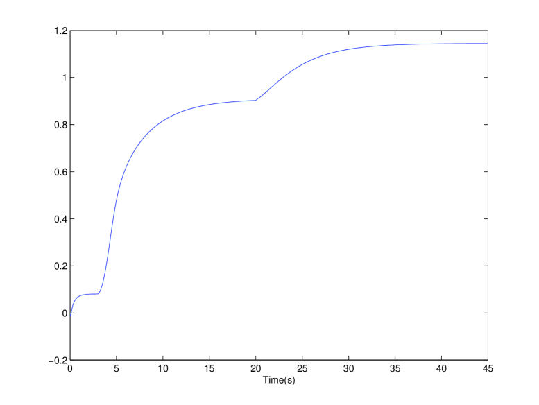
(a) Control

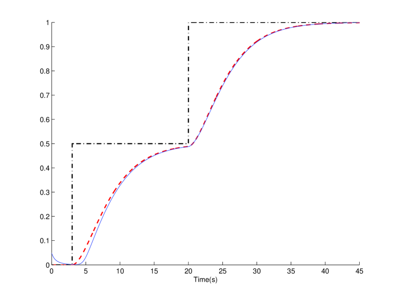
(b) Setpoint (- ., black), Reference (- -, red) and Output (–, blue)

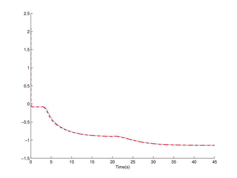
(c) $F$ (- -, red) and $F_{est}$ (–, blue)

Figure 1: $T_{\text{est}}=0.01$s

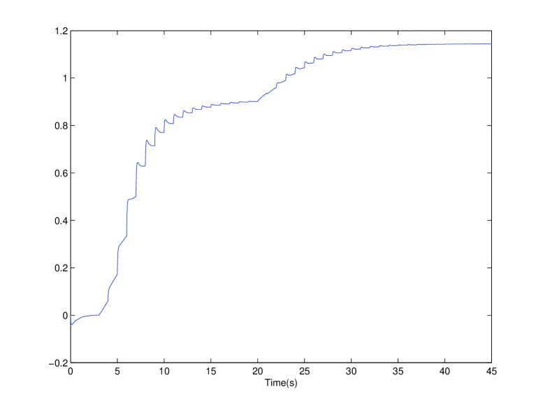
(a) Control

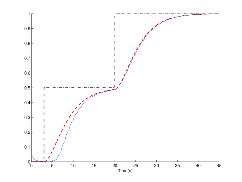
(b) Setpoint (- ., black), Reference (- -, red) and Output (–, blue)

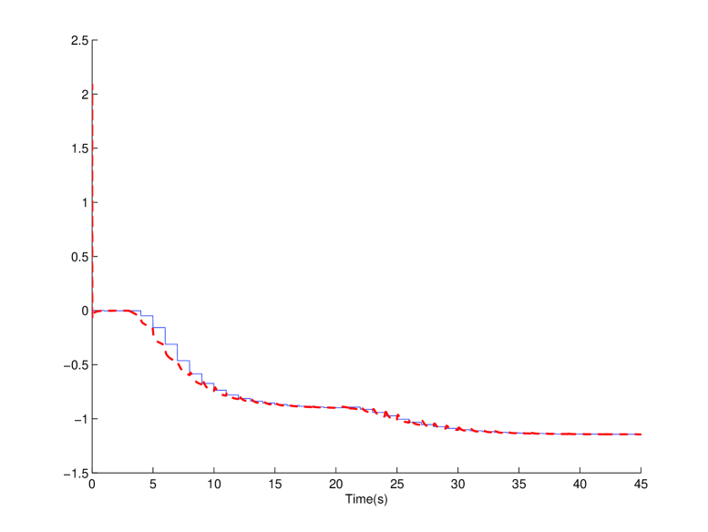
(c) $F$ (- -, red) and $F_{est}$ (–, blue)

Figure 2: $T_{\text{est}}=1\text{s}$

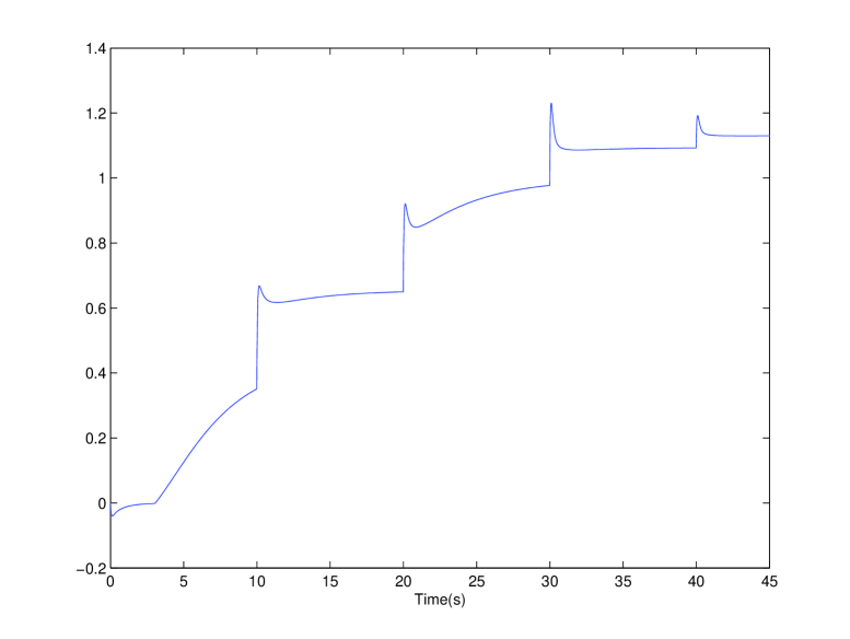
(a) Control

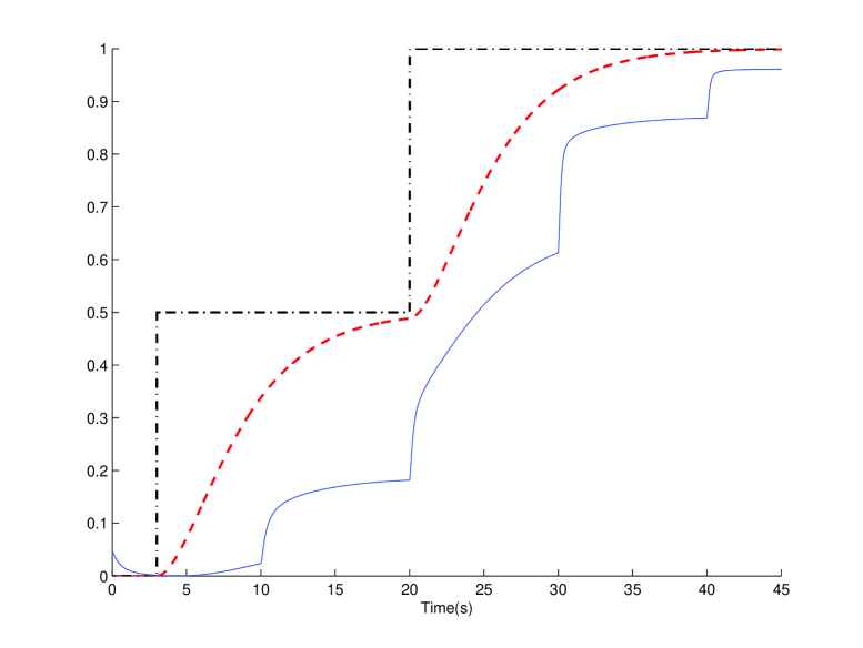
(b) Setpoint (- ., black), Reference (- -, red) and Output (–, blue)

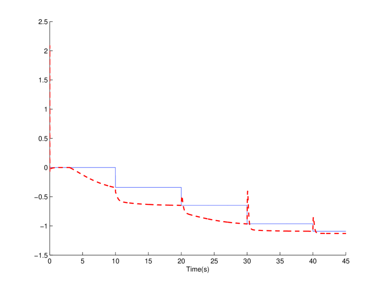
(c) $F$ (- -, red) and $F_{est}$ (–, blue)

Figure 3: $T_{\text{est}}=10\text{s}$

IV-B A linear academic case

IV-B1 Description and control

Consider the unstable single-input single-output linear system

$$2\dot{y}-3y=u$$ (22)

Equation (21) is again used as an ultra-local model. The loop is closed via the iP controller (4) with some suitable gain $K_{P}$. As above, in Section IV-A1, the gain and phase margins are given by Section III-B1. Stability is therefore ensured with a good robustness. Figure 4 displays simulations with $K_{P}=1$, a sampling time period $T_{e}=0.01\text{s}$, and an additive Gaussian corrupting noise $N(0,0.03)$ on the output. The trajectory tracking is excellent.

IV-B2 Robustness with respect to a delayed control

Introduce a time lag $\tau$ in the control transmission. The transfer function of (22) is no more

$$\frac{1}{2s-3}$$

but

$$\frac{e^{-\tau s}}{2s-3}$$

Remark IV.2

Such delays, which might occur in practice, have already been studied in the literature (see, e.g., [22, 23, 27]).

Remark IV.3

Systems with transfer functions of the form

$$T(s)e^{-\tau s}$$

where $T\in\mathbf{R}(s)$ is a rational function, are according to [6] the most usual linear delay single-input single-output systems. It is also well known that they are used for approximating “complex” nonlinear systems without delays (see, e.g., [26]). It has been emphasized in [4] that such approximations are becoming useless when applying model-free control design.

Assume that we are doing the same computations as in Section IV-B1, and, in particular, that $F$ is estimated with the techniques presented in Section II-C. It amounts saying that we are in fact replacing Equation (21) by

$$y(t)=F+u(t-\tau)$$

The open loop transfer function becomes therefore

$$T_{1\tau OLP}=\frac{K_{P}e^{-\tau s}}{s}$$

Solving the equation

$$T_{1\tau OLP}(j\omega)=-1$$

yields

$$\boxed{\tau_{\text{max}}=\frac{\pi}{2K_{P}}}$$

i.e., the maximum admissible time lag for stability.

IV-B3 Computer experiments with delay

Figure 5 displays an excellent stability obtained with a time lag $\tau=0.2\text{s}$ and $K_{P}=1$. Then $\tau_{\text{max}}\simeq 1.57\text{s}$.

With the “high” gain $K_{P}=10$, $\tau_{\text{max}}\simeq 0.16\text{s}$. Stability is then lost as shown by Figure 6.

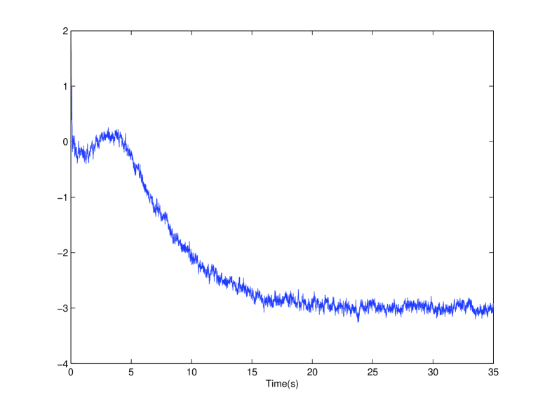
(a) Control

(b) Setpoint (- ., black), Reference (- -, red) and Output (–, blue)

Figure 4: Delay free

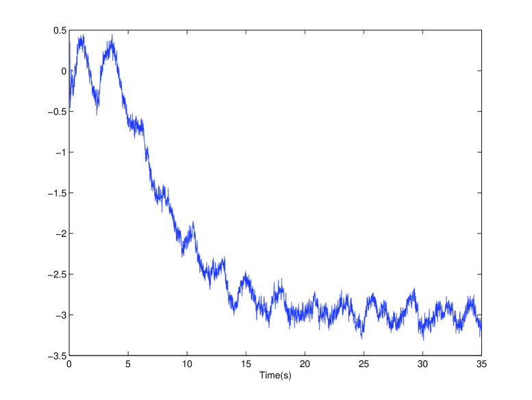
(a) Control

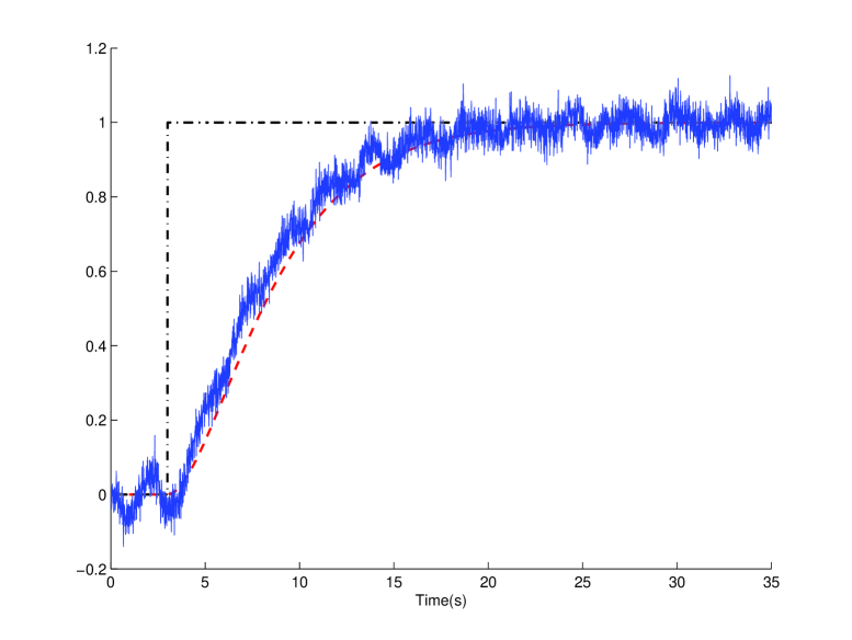
(b) Setpoint (- .,black), Reference (- -, red) and Output (–, blue)

Figure 5: Delayed control – $K_{P}=1$

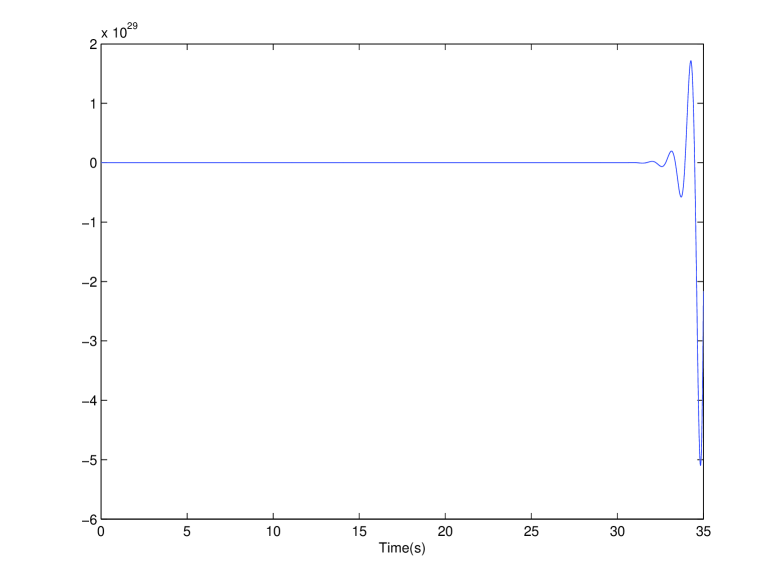
(a) Control

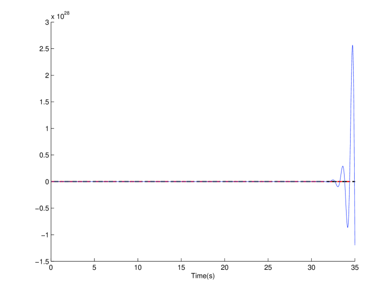
(b) Setpoint (- ., black), Reference (- -, red) and Output (–, blue)

Figure 6: Delayed control – $K_{P}=10$

V Conclusion

We have demonstrated that the calculations related to stability margins may be easily extended to our recent model-free techniques, where they provide some new insight on the robustness with respect to delays. As already discussed in [4], delays, which remain one of the most irritating questions in the model-free setting, do necessitate further investigations. The key point nevertheless in order to ensure satisfactory performances is in our opinion a “good” estimate of $F$. This question, which

• has been summarized in Section II-C,

• might become difficult with very severe corrupting noises and/or a poor time sampling,

seems unfortunately to be far apart from the stability margins techniques.

References

- [1] K.J. Åström, R.M. Murray, Feedback Systems: An Introduction for Scientists and Engineers, Princeton University Press, 2008.
- [2] H. Bourlès, H. Guillard, Commande des systèmes. Performance et robustesse, Ellipses, 2012.
-
[3]
J. De Miras, C. Join, M. Fliess, S. Riachy, S. Bonnet,
Active magnetic bearing: A new step for model-free control,
52nd IEEE Conf. Decision Control, Florence, 2013. Preprint available at
http://hal.archives-ouvertes.fr/hal-00857649/en/ -
[4]
M. Fliess, C. Join,
Model-free control,
Int. J. Control, vol. 86, pp. 2228–2252, 2013. Preprint available at
http://hal.archives-ouvertes.fr/hal-00828135/en/ - [5] M. Fliess, C. Join, H. Sira-Ramírez, Non-linear estimation is easy, Int. J. Model. Identif. Control, vol. 4, pp. 12–27, 2008. Preprint available at http://hal.archives-ouvertes.fr/inria-00158855/en/
- [6] M. Fliess, R. Marquez, H. Mounier, An extension of predictive control, PID regulators and Smith predictors to some linear delay systems, Int. J. Control, vol. 75, pp. 728–743, 2002.
- [7] M. Fliess, H Sira-Ramírez, An algebraic framework for linear identification, ESAIM Control Optimiz. Calc. Variat., vol. 9, pp. 151–168, 2003.
-
[8]
M. Fliess, H. Sira-Ramírez,
Closed-loop parametric identification for continuous-time
linear systems via new algebraic techniques,
in eds. H. Garnier and L. Wang,
Identification of Continuous-time Models from Sampled Data,
Springer, pp. 362–391, 2008. Preprint available at
http://hal.archives-ouvertes.fr/inria-00114958/en/ - [9] O. Föllinger, Regelungstechnik: Einführung in die Methoden und ihre Anwendungen, 8. Aufl., Hüthig, 1994.
- [10] G. F. Franklin, J. D. Powell, A. Emami-Naeini, Feedback Control of Dynamic Systems, 6th ed., Addison-Wesley, 2006.
- [11] F. Golnaraghi, B. C. Kuo, Automatic Control Systems, 9th ed., Prentice-Hall, 2009.
-
[12]
C. Join, F. Chaxel, M. Fliess, “Intelligent” controllers on cheap and small programmable devices,
2nd Int. Conf. Control Fault-Tolerant Syst., Nice, 2013. Preprint available at
http://hal.archives-ouvertes.fr/hal-00845795/en/ -
[13]
C. Join, G. Robert, M. Fliess, Vers une commande sans
modèle pour aménagements hydroélectriques en cascade,
6e Conf. Internat. Francoph. Automat., Nancy, 2010. Preprint available at
http://hal.archives-ouvertes.fr/inria-00460912/en/ -
[14]
F. Lafont, J.-F. Balmat, N. Pessel, M. Fliess, Model-free control and fault accommodation for an experimental greenhouse, Int. Conf. Green Energy Environ. Engin., Sousse, 2014.
Preprint soon available at
http://hal.archives-ouvertes.fr/ - [15] D.Y. Liu, O. Gibaru, W. Perruquetti, Error analysis of Jacobi derivative estimators for noisy signals, Numer. Algor., vol. 58, pp. 53–83, 2011.
- [16] R. Longchamp, Commande numérique des systèmes dynamiques, t. 1, 3e éd., Presses polytechniques et universitaires romandes, 2010.
- [17] R. Madoński, P. Herman, Model-free control of a two-dimensional system based on uncertainty and attenuation, 2nd Int. Conf. Control Fault-Tolerant Syst., Nice, 2013.
- [18] M. Mboup, C. Join, M. Fliess, Numerical differentiation with annihilators in noisy environment, Numer. Algor., vol. 50, pp. 439–467, 2009.
- [19] L. Menhour, B. d’Andréa-Novel, M. Fliess, H. Mounier, Multivariable decoupled longitudinal and lateral vehicle control: A model-free design, 52nd IEEE Conf. Decision Control, Florence, 2013. Preprint available at http://hal.archives-ouvertes.fr/hal-00859444/en/
- [20] L. Michel, W. Michiels, X. Boucher, Model free control of nonlinear power converters, Proc. Canad. Conf. Electric. Comput. Engin., Regina, 2013.
- [21] L. Michel, W. Michiels, X. Boucher, Model free control of microgrids, Proc. Canad. Conf. Electric. Comput. Engin., Regina, 2013.
- [22] R.H. Middleton, D.E. Miller, On the achievable delay margin using LTI control for unstable plants, IEEE Trans. Automat. Control, vol. 52, pp. 1194–1207, 2007.
- [23] S.-I. Niculescu, Delay Effects on Stability: A Robust Control Approach, Springer, 2001.
- [24] J.M. Rodriguez-Fortun, F. Rotella, J. Alfonso, F. Carrillo, J. Orus, Model-free control of a -DOF piezoelectric nanopositioning platform, 52nd IEEE Conf. Decision Control, Florence, 2013.
- [25] R. Sepulchre, M. Jankovic, P. Kokotovic, Constructive Nonlinear Control, Springer, 1997.
- [26] F.G. Shinskey, Process Control Systems, 4th ed., McGraw-Hill, 1996.
- [27] R. Sipahi, S.-I. Niculescu, C.T. Abdallah, W. Michiels, K. Gu, Stability and stabilization of systems with time delay – Limitations and opportunities, IEEE Control Syst. Magaz., vol. 31, pp. 38–65, 2011.
- [28] B.L. van der Waerden, Algebra I, 9. Aufl., Springer, 1993. English translation: Algebra, vol. 1, Springer, 1991.
- [29] J. Wang, M.S. Geamanu, A. Cela, H. Mounier, S.-I. Niculescu, Event driven model free control of quadrotor, IEEE Int. Conf. Control Appli., Hyderabad, 2013.
- [30] Y. Xu, E. Bideaux, D. Thomasset, Robustness study on the model-free control and the control with restricted model of a high performance electro-hydraulic system, 13th Scandin. Int. Conf. Fluid Power, Linköping, 2013.
- [31] K. Yosida, Operational Calculus (translated from the Japanese), Springer, 1984.