MAPK’s networks and their capacity for multistationarity due to toric steady states

Abstract.

Mitogen-activated protein kinase (MAPK) signaling pathways play an essential role in the transduction of environmental stimuli to the nucleus, thereby regulating a variety of cellular processes, including cell proliferation, differentiation and programmed cell death. The components of the MAPK extracellular activated protein kinase (ERK) cascade represent attractive targets for cancer therapy as their aberrant activation is a frequent event among highly prevalent human cancers. MAPK networks are a model for computational simulation, mostly using Ordinary and Partial Differential Equations. Key results showed that these networks can have switch-like behavior, bistability and oscillations. In this work, we consider three representative ERK networks, one with a negative feedback loop, which present a binomial steady state ideal under mass-action kinetics. We therefore apply the theoretical result present in Pérez Millán et al. (2012) to find a set of rate constants that allow two significantly different stable steady states in the same stoichiometric compatibility class for each network. Our approach makes it possible to study certain aspects of the system, such as multistationarity, without relying on simulation, since we do not assume a priori any constant but the topology of the network. As the performed analysis is general it could be applied to many other important biochemical networks.

Keywords: mass-action kinetics, MAPK, signaling networks, toric steady states, multistationarity

1. INTRODUCTION

Mitogen-activated protein kinases (MAPKs) are serine/threonine kinases that play an essential role in signal transduction by modulating gene transcription in the nucleus in response to changes in the cellular environment. MAPKs participate in a number of disease states including chronic inflammation and cancer (Davis, 2000; Kyriakis and Avruch, 2001; Pearson et al., 2001; Schaeffer and Weber, 1999; Zarubin and Han, 2005) as they control key cellular functions, including differentiation, proliferation, migration and apoptosis. In humans, there are several members of the MAPK superfamily which can be divided in groups as each group can be stimulated by a separate protein kinase cascade that includes the sequential activation of a specific MAPK kinase kinase (MAPKKK) and a MAPK kinase (MAPKK), which in turn phosphorylates and activates their downstream MAPKs (Pearson et al., 2001; Turjanski et al., 2007). These signaling modules have been conserved throughout evolution, from plants, fungi, nematodes, insects, to mammals (Widmann et al., 1999). Among the MAPK pathways, the mechanisms governing the activation of ERK2 have been the most extensively studied, the MAPKK is MEK2 and the MAPKKK is RAF which can be activated by RAS. Impeding the function of ERK2 prevents cell proliferation in response to a variety of growth factors (Pagès et al., 1993) and its overactivity is sufficient to transform cells in culture (Mansour et al., 1994). RAS, RAF and MEK2 have been intensively studied for the development of cancer inhibitors with several of them in the market. Indeed, the wealth of available cellular and biochemical information on the nature of the signaling routes that activate MAPK has enabled the use of computational approaches to study MAPK activation, thus becoming a prototype for systems biology studies (Hornberg et al., 2005; Schoeberl et al., 2002).

In the present work, we study the capacity for multistationarity of three systems which involve the activation of a MAPKKK then a MAPKK and finally a MAPK and are of general application but have been proposed previously for the extracellular signal-regulated kinase (ERK) cascade: The first network is the most frequent in the literature (Kholodenko, 2000; Huang and Ferrell, 1996) and is the simple sequential activation. The second one differs from the first one in the phosphatases, which we assume to be equal for the last two layers of the cascades (Fujioka et al., 2006). The third network includes a negative feedback between pRAF and ppERK in which the latter acts as a kinase for the former, producing a new phosphorylated and inactive form Z (Asthagiri and Lauffenburger, 2001; Dougherty et al., 2005; Fritsche-Guenther et al., 2011).

The three networks are summarized in Figure 1.

Figure 1. (A)The ERK network with sequential activation. (B)The ERK network with the same phosphatase for MEK and ERK. (C)The ERK network with a negative feedback.

In general, the existence of (positive) steady states and the capacity for multistationarity of chemical reaction systems is difficult to establish. Even for mass-action systems, the large number of interacting species and the lack of knowledge of the reaction rate constants become major drawbacks. If, however, the steady state ideal of the system is a binomial ideal, it was shown in Pérez Millán et al. (2012) -and recently generalized in Müller et al. (2013)- that these questions can be answered easily. Such systems are said to have toric steady states. For these networks there are necessary and sufficient conditions that allow to decide about multistationarity and they take the form of linear inequality systems (based on previous work by Conradi et al. (2005)).

In this work we show that the three MAPK systems we study have toric steady states, which allows us to exploit the results in Pérez Millán et al. (2012) for determining the existence of positive steady states and the capacity for multistationarity of each system. In fact, each one of the three systems has many choices of rate constants for which they show multistationarity. We present, in the corresponding section, a certain choice of reaction constants for which each system has two different stable steady states. We can moreover conclude that the negative feedback loop is not necessary for the presence of bistability and neither does it prevent the system from this characteristic.

A similar mathematical analysis to signaling networks has been done in previous works. In Conradi and Flockerzi (2012), the authors present necessary and sufficient conditions for multistationarity for mass-action networks with certain structural properties and they also apply their results on some simple ERK cascade networks. The possibility of these networks having toric steady states is not taken into account, while we do consider this characteristic of the systems, thus simplifying the way to prove multistationarity. In Holstein et al. (2013), the authors describe a sign condition that is necessary and sufficient for multistationarity in $n$-site sequential, distributive phosphorylation.

Multistationarity in signaling pathways has also been studied in (Feliu and Wiuf, 2012; Feliu et al., 2012). In the former, the authors study small motifs that repeatedly occur in these pathways. They include examples of a cascade with monostationarity and another with multistationarity, and although different tools are used for this result, it is possible to check that both systems have toric steady states. In Feliu et al. (2012), the focus is on a signaling cascade with $n$ layers and one cycle of post-translational modification at each layer, such that the modified protein of one layer acts as modifier in the next layer, which is shown to have one steady state for fixed total amounts of substrates and enzymes. The analysis is based on variable elimination, but it could be shown that these types of cascades also have toric steady states.

In our work we show that biologically relevant networks have toric steady states, which simplifies the analysis for multistationarity in the sense that it translates the question of finding two different (nonnegative) solutions of a system of polynomial equations into solving systems of linear inequalities.

We give in Section 2 the theoretical background needed to study the capacity for multistationarity of the ERK cascades via toric steady states. The main theorem is adapted from Pérez Millán et al. (2012). We then apply in Section 3 our results to three specific ERK cascades presented in Figure 1: the standard ERK cascade; the ERK cascade with the same phosphatase for the MEK and ERK layers; and the ERK cascade with the same phosphatase for the MEK and ERK layers, and a negative feedback loop. We show that we can find reasonable reaction constants and concentrations that allow to identify two different stable steady states by modeling with ordinary differential equations. An appendix contains the details of the computations.

2. METHODS

We start this section with a brief presentation of the corresponding notation and we finish by revisiting the theorem obtained in Pérez Millán et al. (2012) which we will use to prove the capacity for multistationarity of the general MAPK’s signaling networks with and without feedback. We model our networks under mass-action kinetics.

We introduce the notation with an example: the network for the smallest cascade.

Example 2.1.

For the 2-layer cascade of one cycle of post-translational modification at each layer we have the following network:

where we consider the reactions:

$S_{0}+E\underset{k_{2}}{\overset{k_{1}}{\rightleftarrows}}ES_{0}\overset{k_{3}}{\rightarrow}S_{1}+E$
		$S_{1}+F\underset{k_{5}}{\overset{k_{4}}{\rightleftarrows}}FS_{1}\overset{k_{6}}{\rightarrow}S_{0}+F$
$P_{0}+S_{1}\underset{k_{8}}{\overset{k_{7}}{\rightleftarrows}}S_{1}P_{0}\overset{k_{9}}{\rightarrow}P_{1}+S_{1}$
		$P_{1}+F\underset{k_{11}}{\overset{k_{10}}{\rightleftarrows}}FP_{1}\overset{k_{12}}{\rightarrow}P_{0}+F$

The network in Example 2.1 consists of ten species $S_{0}$, $S_{1}$, $P_{0}$, $P_{1}$, $E$, $F$, $ES_{0}$, $S_{1}P_{0}$, $FS_{1}$ and $FP_{1}$ and twelve complexes: $S_{0}+E$, $ES_{0}$, $S_{1}+E$, $S_{1}+F$, $FS_{1}$, $S_{0}+F$, $P_{0}+S_{1}$, $S_{1}P_{0}$, $P_{1}+S_{1}$, $P_{1}+F$, $FP_{1}$ and $P_{0}+F$. These complexes are connected by $12$ reactions, where each reaction is associated with a rate constant $k_{i}$. In the ordering chosen here, the first reaction would be $S_{0}+E\overset{k_{1}}{\rightarrow}ES_{0}$ with rate constant $k_{1}$. In this reaction, the complex $S_{0}+E$ reacts to the complex $ES_{0}$, hence $S_{0}+E$ is called educt complex and $ES_{0}$ product complex.

We denote with $[\cdot]$ the concentration of a species and then correspond to each concentration a variable $x_{i}$. For example, we can consider:

$x_{1}\leftrightarrow[S_{0}]$, $x_{2}\leftrightarrow[S_{1}]$, $x_{3}\leftrightarrow[P_{0}]$, $x_{4}\leftrightarrow[P_{1}]$, $x_{5}\leftrightarrow[E]$, $x_{6}\leftrightarrow[F]$,

$x_{7}\leftrightarrow[ES_{0}]$, $x_{8}\leftrightarrow[S_{1}P_{0}]$, $x_{9}\leftrightarrow[FS_{1}]$, and $x_{10}\leftrightarrow[FP_{1}]$.

We associate to each species the corresponding canonical vector of $\mathbb{R}^{10}$ ($e_{1}$ to $S_{0}$, $e_{2}$ to $S_{1}$, $\dots$). Then every complex can be represented by the sum of its constituent species (use $y_{i}$ to denote complex vectors): $y_{1}=e_{1}+e_{5}$ for $S_{0}+E$, and so on.

Let us call $s$ the number of species, $m$ the number of complexes, and $r$ the number of reactions. Which, for the running example, would be $s=10$, $m=12$, and $r=12$.

Regarding the equations that describe the dynamics of the biochemical network, under mass-action kinetics, reactions contribute production and consumption terms consisting of monomials like $k_{1}x_{1}x_{5}$ to the rates of formation of the species in the network. This results in a system of ordinary differential equations (ODEs), $dx/dt=f(x;k)$, in which each component rate function $f_{i}(x;k)$ is a polynomial in the state variables $x_{1},x_{2},\cdots,x_{s}\in{\tenbboard R}$ and $k_{1},\cdots,k_{r}\in\mbox{${\tenbboard R}_{>0}$}$ are positive rate constants.

The steady states of such ODEs are then zeros of a set of polynomial equations, $f_{1}(x,k)=0,\cdots,f_{s}(x,k)=0$. Computational algebra and algebraic geometry provide powerful tools for studying these solutions (Cox et al., 1997), and these tools have recently been used to gain new biological insights, for instance in (Manrai and Gunawardena, 2008; Thomson and Gunawardena, 2009a, b; Craciun et al., 2009; Dasgupta et al., 2012). The rate constants can now be treated as symbolic parameters, whose numerical values do not need to be known in advance. The capability to rise above the parameter problem allows more general results to be obtained than can be expected from numerical simulation (Thomson and Gunawardena, 2009b; Karp et al., 2012).

The steady state ideal is defined as the set

$$J~{} =~{}\langle f_{1},f_{2},\dots,f_{s}\rangle$$

$$=\left\{\sum_{i=1}^{s}g_{i}(x)f_{i}(x)\quad|\quad g_{i}(x)\in\mathbb{R}[x_{1},\dots,x_{s}]~{}{\rm for}~{}1\leq i\leq s\right\}.$$

We say that the polynomial dynamical system has toric steady states if $J$ is a binomial ideal (i.e. the ideal $J$ can be generated by binomials) and it admits nonnegative zeros.

We will now introduce some matrices and subspaces that will be useful for studying multistationarity.

The stoichiometric subspace is the vector subspace spanned by the reaction vectors $y_{k}-y_{j}$ (where there is a reaction from complex $y_{j}$ to complex $y_{k}$), and we will denote this space by $\mathcal{S}$. We define the stoichiometric matrix, $N$, in the following way: if the educt complex of the $i$-th reaction is $y_{j}$, and the product complex is $y_{k}$, then the $i$-th column of $N$ is the reaction vector $y_{k}-y_{j}$. Hence, $N$ is an $s\times r$ matrix. Notice that $\mathcal{S}$ is exactly $\textrm{Columnspan}(N)$ (i.e. the subspace generated by the columns of $N$). For the network in Example 2.1, we obtain:

$$N=\left(\begin{array}[]{rrrrrrrrrrrr}-1&1&0&0&0&1&0&0&0&0&0&0\\ 0&0&1&-1&1&0&-1&1&1&0&0&0\\ 0&0&0&0&0&0&-1&1&0&0&0&1\\ 0&0&0&0&0&0&0&0&1&-1&1&0\\ -1&1&1&0&0&0&0&0&0&0&0&0\\ 0&0&0&-1&1&1&0&0&0&-1&1&1\\ 1&-1&-1&0&0&0&0&0&0&0&0&0\\ 0&0&0&0&0&0&1&-1&-1&0&0&0\\ 0&0&0&1&-1&-1&0&0&0&0&0&0\\ 0&0&0&0&0&0&0&0&0&1&-1&-1\end{array}\right)$$

If $\tilde{y}_{i}$ is the vector of the educt complex of the $i$-th reaction, we can define the vector of educt complex monomials

$$\phi(x)~{}:=~{}\left(x^{\tilde{y}_{1}},~{}x^{\tilde{y}_{2}},~{}\ldots,~{}x^{\tilde{y}_{r}}\right)^{t}~{}.$$

In our example, this vector would be:

$$\phi(x)=(x_{1}x_{5},x_{7},x_{7},x_{2}x_{6},x_{9},x_{9},x_{2}x_{3},x_{8},x_{8},x_{4}x_{6},x_{10},x_{10})^{t}.$$

We also define $k\in\mathbb{R}^{r}_{>0}$ to be the vector of reaction rate constants: $k_{i}$ is the rate constant of the $i$-th reaction. A chemical reaction system can then be expressed as:

$$\dot{x}~{}=~{}N\,\operatorname{diag}(k)\,\phi(x)\ .$$

The vector $\dot{x}$ lies in $\mathcal{S}$ for all time $t$. In fact, a trajectory $x(t)$ beginning at a positive vector $x(0)=x^{0}\in{\tenbboard R}^{s}_{>0}$ remains in the stoichiometric compatibility class $(x^{0}+\mathcal{S})\cap\mathbb{R}^{s}_{\geq 0}$ for all positive time. The equations of $x^{0}+\mathcal{S}$ give rise to the conservation relations of the system.

In our example, the conservation relations are:

$$x_{1}+x_{2}+x_{7}+x_{8}+x_{9} =C_{1}$$

(1) $$x_{3}+x_{4}+x_{8}+x_{10} =C_{2}$$

$$x_{5}+x_{7} =C_{3}$$

$$x_{6}+x_{9}+x_{10} =C_{4}$$

These conservation relations in (1) can be translated as the conservation of the total amounts of the first-layer substrate, $S$, the second-layer substrate, $P$, and the enzymes $E$ and $F$, respectively.

A chemical reaction system exhibits multistationarity if there exists a stoichiometric compatibility class with two or more steady states in its relative interior. A system may admit multistationarity for all, some, or no choices of positive rate constants $k_{i}$; if such rate constants exist, then we say that the network has the capacity for multistationarity.

We now recognize that the set $\ker(N)\cap\mathbb{R}_{>0}^{r}$, if nonempty, is the relative interior of the pointed polyhedral cone $\ker(N)\cap\mathbb{R}_{\geq 0}^{r}$. To utilize this cone, we collect a finite set of generators (also called “extreme rays”) of the cone $\ker(N)\cap\mathbb{R}_{\geq 0}^{r}$ as columns of a non-negative matrix $M$.

For network in Example 2.1, a possible matrix $M$ is:

$$M=\left(\begin{array}[]{rrrrrr}1&0&0&0&1&0\\ 1&0&0&0&0&0\\ 0&0&0&0&1&0\\ 0&1&0&0&1&0\\ 0&1&0&0&0&0\\ 0&0&0&0&1&0\\ 0&0&1&0&0&1\\ 0&0&1&0&0&0\\ 0&0&0&0&0&1\\ 0&0&0&1&0&1\\ 0&0&0&1&0&0\\ 0&0&0&0&0&1\end{array}\right)$$

If the steady state ideal $J$ is generated by the binomials $b_{i}x^{\hat{y}_{j}}-b_{j}x^{\hat{y}_{i}}$, let $A\in\mathbb{Z}^{w\times s}$ be a matrix of maximal rank such that $\ker(A)$ equals the span of all the differences $\hat{y}_{j}-\hat{y}_{i}$. For the mass-action system arising from the network in Example 2.1, the ideal $J$ can be generated by the binomials

$$\begin{array}[]{lcl}k_{1}x_{1}x_{5}-(k_{2}+k_{3})x_{7}&&k_{10}x_{4}x_{6}-(k_{11}+k_{12})x_{10}\\ k_{4}x_{2}x_{6}-(k_{5}+k_{6})x_{9}&&k_{3}x_{7}-k_{6}x_{9}\\ k_{7}x_{2}x_{3}-(k_{8}+k_{9})x_{8}&&k_{9}x_{8}-k_{12}x_{10}\end{array}$$

Then, a possible matrix $A$ is

$$A=\left(\begin{array}[]{cccccccccc}1&1&0&1&0&0&1&1&1&1\\ 1&0&1&0&0&1&1&1&1&1\\ 0&0&1&1&0&0&0&1&0&1\\ 0&0&1&0&1&1&1&1&1&1\end{array}\right)$$

We define the sign of a vector $v\in{\tenbboard R}^{s}$ as a vector $sign(v)\in\{-,0,+\}^{s}$ whose $i$-th coordinate is the sign of the $i$-th entry of $v$.

The following theorem from Pérez Millán et al. (2012) is the one that we will use to study the multistationarity of MAPK’s networks with and without feedback.

Theorem 2.2.

Given matrices $A$ and $N$ as above, and nonzero vectors $\alpha\in\textrm{Rowspan}(A)$ and $\sigma\in\textrm{Columnspan}(N)$ with

(2) $$\operatorname{sign}(\alpha)~{}=~{}\operatorname{sign}(\sigma)~{},$$

then two steady states $x^{1}$ and $x^{2}$ and a reaction rate constant vector $k$ that witness multistationarity arise in the following way:

(3) $$\left(x^{1}_{i}\right)_{i=1,\,\ldots,\,s}~{} =~{}\begin{cases}\frac{\sigma_{i}}{e^{\alpha_{i}}-1}\text{, if $\alpha_{i}\neq 0$}\\ \bar{x}_{i}>0\text{, if $\alpha_{i}=0$~{},}\end{cases}$$

where $$\bar{x}_{i}$$ denotes an arbitrary positive number, and

(4) $$x^{2}~{} =~{}\operatorname{diag}(e^{\alpha})\,x^{1}$$

(5) $$k~{} =~{}\operatorname{diag}(\phi(x^{1}))^{-1}\,M\,\lambda~{},$$

for any non-negative vector $\lambda\in\mathbb{R}_{\geq 0}^{p}$ for which $M\,\lambda\in\mathbb{R}_{>0}^{r}$. Conversely, any witness to multistationarity (given by some $x^{1}$, $x^{2}\in\mathbb{R}_{>0}^{s}$, and $k\in\mathbb{R}_{>0}^{r}$) arises from equations  (2), (3), (4), and (5) for some vectors $\alpha\in\textrm{Rowspan}(A)$ and $\sigma\in\textrm{Columnspan}(N)$ that have the same sign.

3. RESULTS

We prove in this section the capacity for multistationarity of three networks that are frequently used to represent the principal kinase transduction pathways in eukaryotic cells, which are the MAPK cascades. The first network is the most frequent in the literature (Kholodenko, 2000; Huang and Ferrell, 1996). The second one differs from the first one in the phosphatases, which we assume to be equal for the last two layers of the cascades (Fujioka et al., 2006). The third network includes a negative feedback between pRAF and ppERK in which the latter acts as a kinase for the former, producing a new phosphorylated and inactive form Z (Asthagiri and Lauffenburger, 2001; Dougherty et al., 2005; Fritsche-Guenther et al., 2011). The three networks are summarized in Figure 1.

We determine that the ERK cascades present toric steady states, and this helps us to prove the capacity for multistationarity of each system. We then determine reaction constants and concentrations that witness multistability. Namely, we analyze the ODEs that arise under mass-action for each network, and we find that the corresponding steady state ideals are binomial. We show, in different appendices, an order for the species of each network, the conservation relations, and binomials that generate the mentioned ideal. We also present a matrix $A$ as in Section 2 for studying multistationarity, and we include the corresponding matrices $N$ and $M$, and vector $\phi(x)$. By solving three different systems of sign equalities, we find vectors $\alpha\in\textrm{Rowspan}(A)$ and $\sigma\in\mathcal{S}$ with $\textrm{sg}(\alpha_{i})=\textrm{sg}(\sigma_{i})$ (for each system) as required by Theorem 2.2 for proving the capacity for multistationarity. With the aid of these vectors, we can build two different steady states and a vector of reaction constants which, according to Theorem 2.2, witness to multistationarity in each case in the corresponding stoichiometric compatibility class defined by the constants (i.e. total amounts). It can be checked that the steady states we find are stable.

In the following subsections we treat each network separately. Numerical computations and simulations in this article were performed with MATLAB, while computations regarding ideals and subspaces were done with Singular.

3.1. The network without feedback and three phosphatases

We start by studying the network for the signaling pathway of ERK without feedback (see Figure 1(A);Kholodenko (2000); Huang and Ferrell (1996)). This network entails $s=22$ species, $m=26$ complexes and $r=30$ reactions which are as follows:

RAF + RAS $\underset{k_{2}}{\overset{k_{1}}{\rightleftarrows}}$ RAS-RAF $\overset{k_{3}}{\rightarrow}$ pRAF + RAS

pRAF + RAFPH $\underset{k_{5}}{\overset{k_{4}}{\rightleftarrows}}$ RAF-RAFPH $\overset{k_{6}}{\rightarrow}$ RAF + RAFPH

MEK + pRAF $\underset{k_{8}}{\overset{k_{7}}{\rightleftarrows}}$ MEK-pRAF $\overset{k_{9}}{\rightarrow}$ pMEK + pRAF $\underset{k_{11}}{\overset{k_{10}}{\rightleftarrows}}$ pMEK-pRAF $\overset{k_{12}}{\rightarrow}$ ppMEK + pRAF

ppMEK+MEKPH $\underset{k_{14}}{\overset{k_{13}}{\rightleftarrows}}$ ppMEK-MEKPH $\overset{k_{15}}{\rightarrow}$ pMEK+MEKPH $\underset{k_{17}}{\overset{k_{16}}{\rightleftarrows}}$ pMEK-MEKPH $\overset{k_{18}}{\rightarrow}$ MEK+MEKPH

ERK+ppMEK $\underset{k_{20}}{\overset{k_{19}}{\rightleftarrows}}$ ERK-ppMEK $\overset{k_{21}}{\rightarrow}$ pERK+ppMEK $\underset{k_{23}}{\overset{k_{22}}{\rightleftarrows}}$ pERK-ppMEK $\overset{k_{24}}{\rightarrow}$ ppERK+ppMEK

ppERK+ERKPH $\underset{k_{26}}{\overset{k_{25}}{\rightleftarrows}}$ ppERK-ERKPH $\overset{k_{27}}{\rightarrow}$ pERK+ERKPH $\underset{k_{29}}{\overset{k_{28}}{\rightleftarrows}}$ pERK-ERKPH $\overset{k_{30}}{\rightarrow}$ ERK+ERKPH

We can prove that the corresponding mass-action system is capable of reaching two significantly different (stable) steady states in the same stoichiometric compatibility class. We refer the reader to Appendix A for the corresponding computations. Figure 2 pictures this feature of the system.

(a)

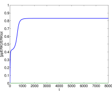
(b)

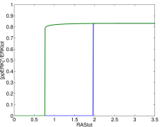
Figure 2. (a) The normalized trajectory of ppERK vs. time for two different initial values in the same stoichiometric compatibility class. The nonzero entries of the initial value for the green curve are [RAF]=12.8629, [MEK]=11.9697, [ERK]=23.3465, [RAS]=2, [RAFPH]=2, [MEKPH]=7.3058 and [ERKPH]=3.2013. The nonzero entries of the initial value for the blue curve are the same except for [MEK]=4.5697 and [ppMEK]=7.4. (b) Dose-response curve for the network without feedback. The horizontal axis represents the total amount of the dose ([RAS]+[RAS-RAF]), and the vertical axis stands for the normalized equilibrium values of [ppERK]. For each value of RAS, the corresponding equilibria belong to the same stoichiometric compatibility class.

3.2. The network without feedback and two phosphatases

We now study the network for the signaling pathway of ERK without feedback and the same phosphatase for both, MEK and ERK (see Figure 1(B); Fujioka et al. (2006)). This network entails $s=21$ species, $m=26$ complexes and $r=30$ reactions which are:

RAF + RAS $\underset{k_{2}}{\overset{k_{1}}{\rightleftarrows}}$ RAS-RAF $\overset{k_{3}}{\rightarrow}$ pRAF + RAS

pRAF + RAFPH $\underset{k_{5}}{\overset{k_{4}}{\rightleftarrows}}$ RAF-RAFPH $\overset{k_{6}}{\rightarrow}$ RAF + RAFPH

MEK + pRAF $\underset{k_{8}}{\overset{k_{7}}{\rightleftarrows}}$ MEK-pRAF $\overset{k_{9}}{\rightarrow}$ pMEK + pRAF $\underset{k_{11}}{\overset{k_{10}}{\rightleftarrows}}$ pMEK-pRAF $\overset{k_{12}}{\rightarrow}$ ppMEK + pRAF

ppMEK+PH $\underset{k_{14}}{\overset{k_{13}}{\rightleftarrows}}$ ppMEK-PH $\overset{k_{15}}{\rightarrow}$ pMEK+PH $\underset{k_{17}}{\overset{k_{16}}{\rightleftarrows}}$ pMEK-PH $\overset{k_{18}}{\rightarrow}$ MEK+PH

ERK+ppMEK $\underset{k_{20}}{\overset{k_{19}}{\rightleftarrows}}$ ERK-ppMEK $\overset{k_{21}}{\rightarrow}$ pERK+ppMEK $\underset{k_{23}}{\overset{k_{22}}{\rightleftarrows}}$ pERK-ppMEK $\overset{k_{24}}{\rightarrow}$ ppERK+ppMEK

ppERK+PH $\underset{k_{26}}{\overset{k_{25}}{\rightleftarrows}}$ ppERK-PH $\overset{k_{27}}{\rightarrow}$ pERK+PH $\underset{k_{29}}{\overset{k_{28}}{\rightleftarrows}}$ pERK-PH $\overset{k_{30}}{\rightarrow}$ ERK+PH

We depict in Figure 3 the hysteresis and bistability this network presents. All the necessary information for this network is presented in Appendix B.

(a)

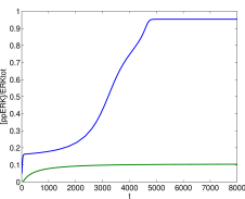
(b)

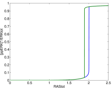
Figure 3. For the network without feedback and the same phosphatase for MEK and ERK. (a) The normalized trajectory of ppERK vs. time for two different initial values in the same stoichiometric compatibility class. The nonzero entries of the initial value for the green curve are [RAF]=4.1738, [MEK]=1.9063, [ERK]=3.7737, [RAS]=2, [RAFPH]=2 and [PH]=1.3995. The nonzero entries of the initial value for the blue curve are the same except for [MEK]=0.0063, [ppMEK]=1.9, [ERK]=3.5237 and [ppERK]=0.25. (b) Dose-response curve for the network without feedback. The horizontal axis represents the total amount of the dose ([RAS]+[RAS-RAF]), and the vertical axis stands for the normalized equilibrium values of [ppERK]. For each value of RAS, the corresponding equilibria belong to the same stoichiometric compatibility class.

3.3. The network with feedback

We now study a network for the signaling pathway of ERK with a negative feedback between pRAF and ppERK in which the latter acts as a kinase for the former, producing a new phosphorylated and inactive form Z (see Figure 1(C);Asthagiri and Lauffenburger (2001); Dougherty et al. (2005); Fritsche-Guenther et al. (2011) ). This network consists of $s=25$ species, $m=32$ complexes and $r=36$ reactions.

RAF + RAS $\underset{k_{2}}{\overset{k_{1}}{\rightleftarrows}}$ RAS-RAF $\overset{k_{3}}{\rightarrow}$ pRAF + RAS

pRAF + RAFPH $\underset{k_{5}}{\overset{k_{4}}{\rightleftarrows}}$ RAF-RAFPH $\overset{k_{6}}{\rightarrow}$ RAF + RAFPH

MEK + pRAF $\underset{k_{8}}{\overset{k_{7}}{\rightleftarrows}}$ MEK-pRAF $\overset{k_{9}}{\rightarrow}$ pMEK + pRAF $\underset{k_{11}}{\overset{k_{10}}{\rightleftarrows}}$ pMEK-pRAF $\overset{k_{12}}{\rightarrow}$ ppMEK + pRAF

ppMEK+PH $\underset{k_{14}}{\overset{k_{13}}{\rightleftarrows}}$ ppMEK-PH $\overset{k_{15}}{\rightarrow}$ pMEK+PH $\underset{k_{17}}{\overset{k_{16}}{\rightleftarrows}}$ pMEK-PH $\overset{k_{18}}{\rightarrow}$ MEK+PH

ERK+ppMEK $\underset{k_{20}}{\overset{k_{19}}{\rightleftarrows}}$ ERK-ppMEK $\overset{k_{21}}{\rightarrow}$ pERK+ppMEK $\underset{k_{23}}{\overset{k_{22}}{\rightleftarrows}}$ pERK-ppMEK $\overset{k_{24}}{\rightarrow}$ ppERK+ppMEK

ppERK+PH $\underset{k_{26}}{\overset{k_{25}}{\rightleftarrows}}$ ppERK-PH $\overset{k_{27}}{\rightarrow}$ pERK+PH $\underset{k_{29}}{\overset{k_{28}}{\rightleftarrows}}$ pERK-PH $\overset{k_{30}}{\rightarrow}$ ERK+PH

pRAF + ppERK $\underset{k_{32}}{\overset{k_{31}}{\rightleftarrows}}$ pRAF-ppERK $\overset{k_{33}}{\rightarrow}$ Z + ppERK

Z + PH2 $\underset{k_{35}}{\overset{k_{34}}{\rightleftarrows}}$ Z-PH2 $\overset{k_{36}}{\rightarrow}$ pRAF + PH2

We can prove that the corresponding mass-action system is capable of reaching two significantly different (stable) steady states in the same stoichiometric compatibility class. We refer the reader to Appendix C for the corresponding computations. Figure 4 pictures this feature of the system.

(a)

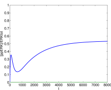
(b)

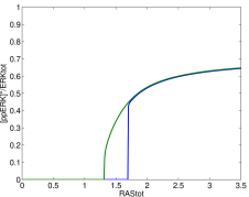
Figure 4. For the network with a negative feedback and the same phosphatase for MEK and ERK. (a) The normalized trajectory of ppERK vs. time for two different initial values in the same stoichiometric compatibility class. The nonzero entries of the initial value for the green curve are [RAF]=12.8629, [MEK]=11.9697, [ERK]=23.3465, [RAS]=2, [RAFPH]=2, [PH]=7.3058 and [PH2]=3.2013. The nonzero entries of the initial value for the blue curve are the same except for [MEK]=4.5697 and [ppMEK]=7.4. (b) Dose-response curve for the network without feedback. The horizontal axis represents the total amount of the dose ([RAS]+[RAS-RAF]), and the vertical axis stands for the normalized equilibrium values of [ppERK]. For each value of RAS, the corresponding equilibria belong to the same stoichiometric compatibility class.

4. DISCUSSION

We have applied a useful algebraic tool for studying the capacity for multistationarity of an important signaling pathway as the MAPK cascade. We included in our analysis three frequent possible networks for describing the MAPK signaling mechanism, which happen to have, under mass-action kinetics, a binomial steady state ideal. This allowed us to translate the question of multistationarity to a system of sign equalities, and so we proved that ERK systems are able to show multistationarity for reasonable choices of rate constants.

The application of computational biology and systems biology is yielding quantitative insight into cellular regulatory phenomena and a a large number of papers have appeared that estimate in-vivo protein concentrations and reaction constants of the MAPK signaling networks (Hornberg et al., 2005). However, there is no agreement about these values and differences of more than two orders of magnitude have appeared (Qiao et al., 2007). In this sense, in our case, any nontrivial solution of the linear inequality system defined by (2) gives two different steady sates and a set of rate constants for which the system has those steady states, and both the steady states and the constants are determined explicitly. Our results highlight that the robustness of the topology also tolerates changes in protein concentrations and rate constants, allowing a similar overall behavior of the network. Concentrations may vary from one organism to another, and kinetic constants can be regulated by different mechanisms as for example the role of scaffolds in MAPK kinase cascades (Kolch, 2005). We also reveal that the MAPK cascades are robust in the sense that neither the differences in phosphatases nor the presence or absence of feedback loops alter the capacity for multistability.

Finally, algebraic methods are proving to be powerful tools for answering questions from biochemical reaction network studies. In particular, they are very useful for addressing matters of steady state characterization (Karp et al., 2012; Müller et al., 2013). The same analysis we performed in the present work could be applied to many other important biochemical networks as long as they present toric steady states. We are currently developing easier (graphical) methods for detecting this characteristic in enzymatic networks, and we plan to improve the computational methods for solving the system of sign equalities defined by Equation (2).

5. ACKNOWLEDGEMENTS

We thank C. Conradi for technical assistance in the first stages of this article and E. Feliu for some useful suggestions.

MPM was partially supported by UBACYT 20020100100242, CONICET PIP 11220110100580 and ANPCyT 2008-0902, Argentina. This research was partially supported by UBACYT 20020110100061BA and ANPCyT 2010-2805. AGT is a staff member of CONICET.

Appendix A The ERK network without feedback.

We present in this appendix the matrices, vectors, constants and corresponding (stable) steady states that prove the capacity for multistationarity for the system without feedback and three different phosphatases for each substrate, presented in Subsection 3.1.

The conservation relations of this system are:

[RAF]+[pRAF]+[RAS-RAF]+[MEK-pRAF]+[pMEK-pRAF]+[pRAF-RAFPH] $$=C_{1}$$

[MEK]+[pMEK]+[ppMEK]+[MEK-pRAF]+[pMEK-pRAF]+[ERK-ppMEK]+

+[pERK-ppMEK]+[ppMEK-MEKPH]+[pMEK-MEKPH] $$=C_{2}$$

[ERK]+[pERK]+[ppERK]+[ERK-ppMEK]+[pERK-ppMEK]+

+[ppERK-ERKPH]+[pERK-ERKPH] $$=C_{3}$$

[RAS]+[RAS-RAF] $$=C_{4}$$

[RAFPH]+[RAF-RAFPH] $$=C_{5}$$

[MEKPH]+[ppMEK-MEKPH]+[pMEK-MEKPH] $$=C_{6}$$

[ERKPH]+[ppERK-ERKPH]+[pERK-ERKPH] $$=C_{7}$$

Where $C_{1},\dots,C_{7}$ usually stand, respectively, for [RAF]_tot, [MEK]_tot, [ERK]_tot, [RAS]_tot, [RAFPH]_tot, [MEKPH]_tot, and [ERKPH]_tot, the total amounts of the corresponding species.

Under mass-action kinetics, the steady state ideal for this network is binomial. In fact, if we consider the following order of the species:

$x_{1}\leftrightarrow[RAF]$, $x_{2}\leftrightarrow[pRAF]$, $x_{3}\leftrightarrow[MEK]$, $x_{4}\leftrightarrow[pMEK]$, $x_{5}\leftrightarrow[ppMEK]$,

$x_{6}\leftrightarrow[ERK]$, $x_{7}\leftrightarrow[pERK]$, $x_{8}\leftrightarrow[ppERK]$, $x_{9}\leftrightarrow[RAS]$, $x_{10}\leftrightarrow[RAFPH]$,

$x_{11}\leftrightarrow[MEKPH]$, $x_{12}\leftrightarrow[ERKPH]$ $x_{13}\leftrightarrow[RAS-RAF]$,

$x_{14}\leftrightarrow[MEK-pRAF]$, $x_{15}\leftrightarrow[pMEK-pRAF]$, $x_{16}\leftrightarrow[ERK-ppMEK]$,

$x_{17}\leftrightarrow[pERK-ppMEK]$, $x_{18}\leftrightarrow[RAF-RAFPH]$,

$x_{19}\leftrightarrow[ppMEK-MEKPH]$, $x_{20}\leftrightarrow[pMEK-MEKPH]$,

$x_{21}\leftrightarrow[ppERK-ERKPH]$, $x_{22}\leftrightarrow[pERK-ERKPH]$,

we obtain these binomials that generate the steady state ideal:

${(k_{2}+k_{3})}x_{13}-{k_{1}}x_{1}x_{9}$		${(k_{5}+k_{6})}x_{18}-{k_{4}}x_{2}x_{10}$		$k_{3}x_{13}-k_{6}x_{18}$
${(k_{8}+k_{9})}x_{14}-{k_{7}}x_{2}x_{3}$		${(k_{14}+k_{15})}x_{19}-{k_{13}}x_{5}x_{11}$		$k_{9}x_{14}-k_{18}x_{20}$
${(k_{11}+k_{12})}x_{15}-{k_{10}}x_{2}x_{4}$		${(k_{17}+k_{18})}x_{20}-{k_{16}}x_{4}x_{11}$		$k_{12}x_{15}-k_{15}x_{19}$
${(k_{20}+k_{21})}x_{16}-{k_{19}}x_{5}x_{6}$		${(k_{26}+k_{27})}x_{21}-{k_{25}}x_{8}x_{12}$		$k_{21}x_{16}-k_{30}x_{22}$
${(k_{23}+k_{24})}x_{17}-{k_{22}}x_{5}x_{7}$		${(k_{29}+k_{30})}x_{22}-{k_{28}}x_{7}x_{12}$		$k_{24}x_{17}-k_{27}x_{21}$

We the aid of the matrices and vectors we show below, we found two steady states for this network. The first one, $x^{1}$, is approximately:

$[RAF]=3.9412$,		$[pRAF]=3.9412$,
$[MEK]=0.0005$,		$[pMEK]=0.0439$,
$[ppMEK]=1.8241$,		$[ERK]=0.0084$,
$[pERK]=1.1512$,		${\color[rgb]{1,0,0}[ppERK]=19.3999}$,
$[RAS]=0.4048$,		$[RAFPH]=0.4048$,
$[MEKPH]=0.0099$,		$[ERKPH]=1.4295$
$[RAS-RAF]=1.5952$,		$[MEK-pRAF]=0.0531$,
$[pMEK-pRAF]=1.7369$,		$[ERK-ppMEK]=0.0237$,
$[pERK-ppMEK]=0.9915$,		$[RAF-RAFPH]=1.5952$,
$[ppMEK-MEKPH]=7.2949$,		$[pMEK-MEKPH]=0.0010$,
$[ppERK-ERKPH]=0.9915$,		$[pERK-ERKPH]=0.7803$

The second steady state, $x^{2}$, is then built as:

$[RAF]=0.4715$,		$[pRAF]=0.4715$,
$[MEK]=0.8619$,		$[pMEK]=0.0126$,
$[ppMEK]=0.0001$,		$[ERK]=23.1647$,
$[pERK]=0.0724$,		${\color[rgb]{1,0,0}[ppERK]=0.00003}$,
$[RAS]=1.3591$,		$[RAFPH]=1.3591$,
$[MEKPH]=6.8520$,		$[ERKPH]=3.0951$
$[RAS-RAF]=0.6409$,		$[MEK-pRAF]=10.5784$,
$[pMEK-pRAF]=0.0597$,		$[ERK-ppMEK]=0.0032$,
$[pERK-ppMEK]=0.0001$,		$[RAF-RAFPH]=0.6409$,
$[ppMEK-MEKPH]=0.2506$,		$[pMEK-MEKPH]=0.2032$,
$[ppERK-ERKPH]=0.0001$,		$[pERK-ERKPH]=0.1062$

Both steady states can be shown to be stable, and the total amounts defining the corresponding stoichiometric compatibility class are

[RAF]${}_{tot}=12.8629,$ [MEK]${}_{tot}=11.9697,$ [ERK]${}_{tot}=23.3465,$ [RAS]${}_{tot}=2,$ [RAFPH]${}_{tot}=2,$ [MEKPH]${}_{tot}=7.3058,$ and [ERKPH]${}_{tot}=3.2013.$

The rate constants that arise for the system to have the previous stable steady states are the following:

$k_{1}=1.2537,$	$k_{2}=0.6269,$	$k_{3}=0.6269,$	$k_{4}=1.2537,$	$k_{5}=0.6269,$
$k_{6}=0.6269,$	$k_{7}=5.3900,$	$k_{8}=0.1882,$	$k_{9}=0.0188,$	$k_{10}=5.8335,$
$k_{11}=0.5757,$	$k_{12}=0.0058,$	$k_{13}=6.1030,$	$k_{14}=0.0137,$	$k_{15}=0.0014,$
$k_{16}=4.6076,$	$k_{17}=0.9800,$	$k_{18}=0.9800,$	$k_{19}=7.1500,$	$k_{20}=0.4218,$
$k_{21}=4.2181,$	$k_{22}=0.9524,$	$k_{23}=1.0086,$	$k_{24}=1.0086,$	$k_{25}=0.0721,$
$k_{26}=1.0086,$	$k_{27}=1.0086,$	$k_{28}=0.6684,$	$k_{29}=1.2816,$	$k_{30}=0.0128.$

The matrix $A$ we chose from the binomials above can be found below. The vectors $\alpha\in\textrm{Rowspan}(A)$ and $\sigma\in\mathcal{S}$ with $\textrm{sg}(\alpha_{i})=\textrm{sg}(\sigma_{i})$ for $i=1,\dots,22$ that we found are:

$$\alpha=( {\scriptstyle-2.1233,\,-2.1233,\,7.4172,\,-1.2477,\,-9.9127,\,7.9181,\,-2.7671,\,-13.4522,\,1.2113,\,1.2113,\,6.5417,\,}$$

$${\scriptstyle 0.7725,\,-0.9120,\,5.2940,\,-3.3710,\,-1.9946,\,-12.6797,\,-0.9120,\,-3.3710,\,5.2940,\,-12.6797,\,-1.9946}),$$

$$\sigma=( {\scriptstyle-3.4697,\,-3.4697,\,0.8613,\,-0.0313,\,-1.8240,\,23.1563,\,-1.0789,\,-19.3998,\,0.9544,\,0.9544,\,6.8421,\,}$$

$${\scriptstyle 1.6656,\,-0.9544,\,10.5253,\,-1.6772,\,-0.0205,\,-0.9915,\,-0.9544,\,-7.0443,\,0.2022,\,-0.9915,\,-0.6741}),$$

where the sign pattern is

$\text{sign}(\alpha)=\text{sign}(\sigma)=({\scriptstyle-,\,-,\,+,\,-,\,-,\,+,\,-,\,-,\,+,\,+,\,+,\,+,\,-,\,+,\,-,\,-,\,-,\,-,\,-,\,+,\,-,\,-}).$

We present below the matrices $N$ and $M$, and vector $\lambda$ where the order for the reactions is defined by the subindices of the rate constants.

$M=\left(\begin{array}[]{ccccccccccccccc}1&1&0&0&0&0&0&0&0&0&0&0&0&0&0\\ 1&0&0&0&0&0&0&0&0&0&0&0&0&0&0\\ 0&1&0&0&0&0&0&0&0&0&0&0&0&0&0\\ 0&1&1&0&0&0&0&0&0&0&0&0&0&0&0\\ 0&0&1&0&0&0&0&0&0&0&0&0&0&0&0\\ 0&1&0&0&0&0&0&0&0&0&0&0&0&0&0\\ 0&0&0&1&1&0&0&0&0&0&0&0&0&0&0\\ 0&0&0&1&0&0&0&0&0&0&0&0&0&0&0\\ 0&0&0&0&1&0&0&0&0&0&0&0&0&0&0\\ 0&0&0&0&0&1&1&0&0&0&0&0&0&0&0\\ 0&0&0&0&0&1&0&0&0&0&0&0&0&0&0\\ 0&0&0&0&0&0&1&0&0&0&0&0&0&0&0\\ 0&0&0&0&0&0&1&1&0&0&0&0&0&0&0\\ 0&0&0&0&0&0&0&1&0&0&0&0&0&0&0\\ 0&0&0&0&0&0&1&0&0&0&0&0&0&0&0\\ 0&0&0&0&1&0&0&0&1&0&0&0&0&0&0\\ 0&0&0&0&0&0&0&0&1&0&0&0&0&0&0\\ 0&0&0&0&1&0&0&0&0&0&0&0&0&0&0\\ 0&0&0&0&0&0&0&0&0&1&1&0&0&0&0\\ 0&0&0&0&0&0&0&0&0&1&0&0&0&0&0\\ 0&0&0&0&0&0&0&0&0&0&1&0&0&0&0\\ 0&0&0&0&0&0&0&0&0&0&0&1&1&0&0\\ 0&0&0&0&0&0&0&0&0&0&0&1&0&0&0\\ 0&0&0&0&0&0&0&0&0&0&0&0&1&0&0\\ 0&0&0&0&0&0&0&0&0&0&0&0&1&1&0\\ 0&0&0&0&0&0&0&0&0&0&0&0&0&1&0\\ 0&0&0&0&0&0&0&0&0&0&0&0&1&0&0\\ 0&0&0&0&0&0&0&0&0&0&1&0&0&0&1\\ 0&0&0&0&0&0&0&0&0&0&0&0&0&0&1\\ 0&0&0&0&0&0&0&0&0&0&1&0&0&0&0\end{array}\right)$

$\lambda=(1,1,1,0.01,0.001,1,0.01,0.1,0.001,0.01,0.1,1,1,1,1)$.

$A=\left(\begin{array}[]{rrrrrrrrrrrrrrrrrrrrrr}-1&0&0&0&0&0&0&0&1&0&0&0&0&0&0&0&0&0&0&0&0&0\\ 0&1&-1&-1&-1&2&1&0&0&-1&1&0&0&0&0&1&0&0&0&0&0&1\\ 0&0&1&0&-1&2&1&0&0&0&1&0&0&1&0&1&0&0&0&1&0&1\\ 0&0&0&1&2&-4&-2&0&0&0&-1&0&0&0&1&-2&0&0&1&0&0&-2\\ 0&0&0&0&0&1&0&-1&0&0&0&1&0&0&0&1&0&0&0&0&0&1\\ 0&0&0&0&0&0&1&2&0&0&0&-1&0&0&0&0&1&0&0&0&1&0\\ 0&0&0&0&0&0&0&0&1&1&0&0&1&0&0&0&0&1&0&0&0&0\end{array}\right)$

$N=\left(\begin{array}[]{cccccccccccccccccccccccccccccc}-1&1&0&0&0&1&0&0&0&0&0&0&0&0&0&0&0&0&0&0&0&0&0&0&0&0&0&0&0&0\\ 0&0&1&-1&1&0&-1&1&1&-1&1&1&0&0&0&0&0&0&0&0&0&0&0&0&0&0&0&0&0&0\\ 0&0&0&0&0&0&-1&1&0&0&0&0&0&0&0&0&0&1&0&0&0&0&0&0&0&0&0&0&0&0\\ 0&0&0&0&0&0&0&0&1&-1&1&0&0&0&1&-1&1&0&0&0&0&0&0&0&0&0&0&0&0&0\\ 0&0&0&0&0&0&0&0&0&0&0&1&-1&1&0&0&0&0&-1&1&1&-1&1&1&0&0&0&0&0&0\\ 0&0&0&0&0&0&0&0&0&0&0&0&0&0&0&0&0&0&-1&1&0&0&0&0&0&0&0&0&0&1\\ 0&0&0&0&0&0&0&0&0&0&0&0&0&0&0&0&0&0&0&0&1&-1&1&0&0&0&1&-1&1&0\\ 0&0&0&0&0&0&0&0&0&0&0&0&0&0&0&0&0&0&0&0&0&0&0&1&-1&1&0&0&0&0\\ -1&1&1&0&0&0&0&0&0&0&0&0&0&0&0&0&0&0&0&0&0&0&0&0&0&0&0&0&0&0\\ 0&0&0&-1&1&1&0&0&0&0&0&0&0&0&0&0&0&0&0&0&0&0&0&0&0&0&0&0&0&0\\ 0&0&0&0&0&0&0&0&0&0&0&0&-1&1&1&-1&1&1&0&0&0&0&0&0&0&0&0&0&0&0\\ 0&0&0&0&0&0&0&0&0&0&0&0&0&0&0&0&0&0&0&0&0&0&0&0&-1&1&1&-1&1&1\\ 1&-1&-1&0&0&0&0&0&0&0&0&0&0&0&0&0&0&0&0&0&0&0&0&0&0&0&0&0&0&0\\ 0&0&0&0&0&0&1&-1&-1&0&0&0&0&0&0&0&0&0&0&0&0&0&0&0&0&0&0&0&0&0\\ 0&0&0&0&0&0&0&0&0&1&-1&-1&0&0&0&0&0&0&0&0&0&0&0&0&0&0&0&0&0&0\\ 0&0&0&0&0&0&0&0&0&0&0&0&0&0&0&0&0&0&1&-1&-1&0&0&0&0&0&0&0&0&0\\ 0&0&0&0&0&0&0&0&0&0&0&0&0&0&0&0&0&0&0&0&0&1&-1&-1&0&0&0&0&0&0\\ 0&0&0&1&-1&-1&0&0&0&0&0&0&0&0&0&0&0&0&0&0&0&0&0&0&0&0&0&0&0&0\\ 0&0&0&0&0&0&0&0&0&0&0&0&1&-1&-1&0&0&0&0&0&0&0&0&0&0&0&0&0&0&0\\ 0&0&0&0&0&0&0&0&0&0&0&0&0&0&0&1&-1&-1&0&0&0&0&0&0&0&0&0&0&0&0\\ 0&0&0&0&0&0&0&0&0&0&0&0&0&0&0&0&0&0&0&0&0&0&0&0&1&-1&-1&0&0&0\\ 0&0&0&0&0&0&0&0&0&0&0&0&0&0&0&0&0&0&0&0&0&0&0&0&0&0&0&1&-1&-1\end{array}\right)$

Appendix B The ERK network without feedback and two phosphatases.

We present in this appendix the matrices, vectors, constants and corresponding (stable) steady states that prove the capacity for multistationarity for the system without feedback and two phosphatases, presented in Subsection 3.2.

The conservation relations of this system are:

[RAF]+[pRAF]+[RAS-RAF]+[MEK-pRAF]+[pMEK-pRAF]+

+[pRAF-RAFPH] $$=C_{1}$$

[MEK]+[pMEK]+[ppMEK]+[MEK-pRAF]+[pMEK-pRAF]+

+[ERK-ppMEK]+[pERK-ppMEK]+[ppMEK-PH]+[pMEK-PH] $$=C_{2}$$

[ERK]+[pERK]+[ppERK]+[ERK-ppMEK]+[pERK-ppMEK]+

+[ppERK-PH]+[pERK-PH] $$=C_{3}$$

[RAS]+[RAS-RAF] $$=C_{4}$$

[RAFPH]+[RAF-RAFPH] $$=C_{5}$$

[PH]+[ppMEK-PH]+[pMEK-PH]+[ppERK-PH]+[pERK-PH] $$=C_{6}$$

Under mass-action kinetics, the steady state ideal for this network is binomial. In fact, if we consider the following order of the species:

$x_{1}\leftrightarrow[RAF]$, $x_{2}\leftrightarrow[pRAF]$, $x_{3}\leftrightarrow[MEK]$, $x_{4}\leftrightarrow[pMEK]$, $x_{5}\leftrightarrow[ppMEK]$,

$x_{6}\leftrightarrow[ERK]$, $x_{7}\leftrightarrow[pERK]$, $x_{8}\leftrightarrow[ppERK]$, $x_{9}\leftrightarrow[RAS]$, $x_{10}\leftrightarrow[RAFPH]$,

$x_{11}\leftrightarrow[PH]$, $x_{12}\leftrightarrow[RAS-RAF]$, $x_{13}\leftrightarrow[MEK-pRAF]$,

$x_{14}\leftrightarrow[pMEK-pRAF]$, $x_{15}\leftrightarrow[ERK-ppMEK]$, $x_{16}\leftrightarrow[pERK-ppMEK]$,

$x_{17}\leftrightarrow[RAF-RAFPH]$, $x_{18}\leftrightarrow[ppMEK-PH]$, $x_{19}\leftrightarrow[pMEK-PH]$,

$x_{20}\leftrightarrow[ppERK-PH]$, $x_{21}\leftrightarrow[pERK-PH]$,

we obtain these binomials that generate the steady state ideal:

${(k_{2}+k_{3})}x_{12}-{k_{1}}x_{1}x_{9}$		${(k_{5}+k_{6})}x_{17}-{k_{4}}x_{2}x_{10}$		$k_{3}x_{12}-k_{6}x_{17}$
${(k_{8}+k_{9})}x_{13}-{k_{7}}x_{2}x_{3}$		${(k_{14}+k_{15})}x_{18}-{k_{13}}x_{5}x_{11}$		$k_{9}x_{13}-k_{18}x_{19}$
${(k_{11}+k_{12})}x_{14}-{k_{10}}x_{2}x_{4}$		${(k_{17}+k_{18})}x_{19}-{k_{16}}x_{4}x_{11}$		$k_{12}x_{14}-k_{15}x_{18}$
${(k_{20}+k_{21})}x_{15}-{k_{19}}x_{5}x_{6}$		${(k_{26}+k_{27})}x_{20}-{k_{25}}x_{8}x_{11}$		$k_{21}x_{15}-k_{30}x_{21}$
${(k_{23}+k_{24})}x_{16}-{k_{22}}x_{5}x_{7}$		${(k_{29}+k_{30})}x_{21}-{k_{28}}x_{7}x_{11}$		$k_{24}x_{16}-k_{27}x_{20}$

We the aid of the matrices and vectors we show below, we found two steady states for this network. The first one, $x^{1}$, is approximately:

$[RAF]=1$,		$[pRAF]=1$,
$[MEK]=0.0939$,		$[pMEK]=0.1582$,
$[ppMEK]=0.1019$,		$[ERK]=0$,
$[pERK]=0.0116$,		${\color[rgb]{1,0,0}[ppERK]=3.5988}$,
$[RAS]=1$,		$[RAFPH]=1$,
$[PH]0.0210=$,		$[RAS-RAF]=1$,
$[MEK-pRAF]=0.0157$,		$[pMEK-pRAF]=0.1582$,
$[ERK-ppMEK]=0$,		$[pERK-ppMEK]=0.0816$,
$[RAF-RAFPH]=1$,		$[ppMEK-PH]=1.2656$,
$[pMEK-PH]=0.0313$,		$[ppERK-PH]=0.0816$,
$[pERK-PH]=0$

The second steady state, $x^{2}$, would then be:

$[RAF]=1$,		$[pRAF]=1$,
$[MEK]=0.6939$,		$[pMEK]=0.0582$,
$[ppMEK]=0.0019$,		$[ERK]=1.4000$,
$[pERK]=1.4116$,		${\color[rgb]{1,0,0}[ppERK]=0.3988}$,
$[RAS]=1$,		$[RAFPH]=1$,
$[PH]=0.4210$,		$[RAS-RAF]=1$,
$[MEK-pRAF]=0.1157$,		$[pMEK-pRAF]=0.0582$,
$[ERK-ppMEK]=0.1$,		$[pERK-ppMEK]=0.1816$,
$[RAF-RAFPH]=1$,		$[ppMEK-MEKPH]=0.4656$,
$[pMEK-MEKPH]=0.2313$,		$[ppERK-ERKPH]=0.1816$,
$[pERK-ERKPH]=0.1$

Both steady states can be shown to be stable, and the total amounts defining the corresponding stoichiometric compatibility class are

[RAF]${}_{tot}=4.1738,$ [MEK]${}_{tot}=1.9063,$ [ERK]${}_{tot}=3.7737,$ [RAS]${}_{tot}=2,$ [RAFPH]${}_{tot}=2,$ and [PH]${}_{tot}=1.3995.$

The rate constants that arise for the system to have the previous stable steady states are the following:

$k_{1}=2,$	$k_{2}=1,$	$k_{3}=1,$	$k_{4}=2,$
$k_{5}=1,$	$k_{6}=1,$	$k_{7}=1.1713,$	$k_{8}=6.3891,$
$k_{9}=0.6389,$	$k_{10}=6.9533,$	$k_{11}=6.3212,$	$k_{12}=0.6321,$
$k_{13}=93.6799,$	$k_{14}=0.0790,$	$k_{15}=0.0790,$	$k_{16}=6.0322,$
$k_{17}=0.3195,$	$k_{18}=0.3195,$	$k_{19}=18.6873,$	$k_{20}=0.2440,$
$k_{21}=0.2440,$	$k_{22}=16.9005,$	$k_{23}=0.1226,$	$k_{24}=0.1226,$
$k_{25}=13.3910,$	$k_{26}=12.2554,$	$k_{27}=0.1226,$	$k_{28}=4.1482,$
$k_{29}=24.3960,$	$k_{30}=0.2440.$

The matrix $A$ we chose from the binomials above is depicted below. The vectors $\alpha\in\textrm{Rowspan}(A)$ and $\sigma\in\mathcal{S}$ with $\textrm{sg}(\alpha_{i})=\textrm{sg}(\sigma_{i})$ for $i=1,\dots,21$ that we found are

$$\alpha= ({\scriptstyle 0,\;0,\;2,\;-1,\;-4,\;11.8,\;4.8,\;-2.2,\;0,\;0,\;3,\;0,\;2,\;-1,\;7.8,\;0.8,\;0,\;-1,\;2,\;0.8,\;7.8}),$$

$$\sigma= ({\scriptstyle 0,\;0,\;0.6,\;-0.1,\;-0.1,\;1.4,1.4,\;-3.2,\;0,\;0,\;0.4,\;0,\;0.1,\;-0.1,\;0.1,\;0.1,\;0,\;-0.8,\;0.2,\;0.1,\;0.1}),$$

where the sign pattern is

$\text{sign}(\alpha)=\text{sign}(\sigma)=({\scriptstyle 0,\,0,\,+,\,-,\,-,\,+,\,+,\,-,\,0,\,0,\,+,\,0,\,+,\,-,\,+,\,+,\,0,\,-,\,+,\,+,\,+})$.

We present below the matrices $N$ and $M$, and vector $\lambda$ where the order for the reactions is defined by the subindices of the rate constants.

$M=\left(\begin{array}[]{ccccccccccccccc}1&0&0&0&0&0&0&0&0&0&1&0&0&0&0\\ 1&0&0&0&0&0&0&0&0&0&0&0&0&0&0\\ 0&0&0&0&0&0&0&0&0&0&1&0&0&0&0\\ 0&1&0&0&0&0&0&0&0&0&1&0&0&0&0\\ 0&1&0&0&0&0&0&0&0&0&0&0&0&0&0\\ 0&0&0&0&0&0&0&0&0&0&1&0&0&0&0\\ 0&0&0&0&1&0&0&0&0&0&0&1&0&0&0\\ 0&0&0&0&1&0&0&0&0&0&0&0&0&0&0\\ 0&0&0&0&0&0&0&0&0&0&0&1&0&0&0\\ 0&0&1&0&0&0&0&0&0&0&0&0&1&0&0\\ 0&0&1&0&0&0&0&0&0&0&0&0&0&0&0\\ 0&0&0&0&0&0&0&0&0&0&0&0&1&0&0\\ 0&0&0&1&0&0&0&0&0&0&0&0&1&0&0\\ 0&0&0&1&0&0&0&0&0&0&0&0&0&0&0\\ 0&0&0&0&0&0&0&0&0&0&0&0&1&0&0\\ 0&0&0&0&0&1&0&0&0&0&0&1&0&0&0\\ 0&0&0&0&0&1&0&0&0&0&0&0&0&0&0\\ 0&0&0&0&0&0&0&0&0&0&0&1&0&0&0\\ 0&0&0&0&0&0&1&0&0&0&0&0&0&0&1\\ 0&0&0&0&0&0&1&0&0&0&0&0&0&0&0\\ 0&0&0&0&0&0&0&0&0&0&0&0&0&0&1\\ 0&0&0&0&0&0&0&1&0&0&0&0&0&1&0\\ 0&0&0&0&0&0&0&1&0&0&0&0&0&0&0\\ 0&0&0&0&0&0&0&0&0&0&0&0&0&1&0\\ 0&0&0&0&0&0&0&0&1&0&0&0&0&1&0\\ 0&0&0&0&0&0&0&0&1&0&0&0&0&0&0\\ 0&0&0&0&0&0&0&0&0&0&0&0&0&1&0\\ 0&0&0&0&0&0&0&0&0&1&0&0&0&0&1\\ 0&0&0&0&0&0&0&0&0&1&0&0&0&0&0\\ 0&0&0&0&0&0&0&0&0&0&0&0&0&0&1\end{array}\right)$

$\lambda=(1,1,1,0.1,0.1,0.01,0.00001,0.01,1,0.001,1,0.01,0.1,0.01,0.00001)$.

$A=\left(\begin{array}[]{rrrrrrrrrrrrrrrrrrrrr}-1&0&0&0&0&0&0&0&1&0&0&0&0&0&0&0&0&0&0&0&0\\ 0&1&-1&-1&-1&3&1&-1&0&-1&1&0&0&0&2&0&0&0&0&0&2\\ 0&0&0&0&0&1&1&1&0&0&0&0&0&0&1&1&0&0&0&1&1\\ 1&0&0&0&0&0&0&0&0&1&0&1&0&0&0&0&1&0&0&0&0\\ 0&1&-1&0&1&-2&-1&0&0&-1&0&0&0&1&-1&0&0&1&0&0&-1\\ 0&-1&2&1&0&0&0&0&0&1&0&0&1&0&0&0&0&0&1&0&0\\ \end{array}\right)$

$N=\left(\begin{array}[]{cccccccccccccccccccccccccccccc}-1&1&0&0&0&1&0&0&0&0&0&0&0&0&0&0&0&0&0&0&0&0&0&0&0&0&0&0&0&0\\ 0&0&1&-1&1&0&-1&1&1&-1&1&1&0&0&0&0&0&0&0&0&0&0&0&0&0&0&0&0&0&0\\ 0&0&0&0&0&0&-1&1&0&0&0&0&0&0&0&0&0&1&0&0&0&0&0&0&0&0&0&0&0&0\\ 0&0&0&0&0&0&0&0&1&-1&1&0&0&0&1&-1&1&0&0&0&0&0&0&0&0&0&0&0&0&0\\ 0&0&0&0&0&0&0&0&0&0&0&1&-1&1&0&0&0&0&-1&1&1&-1&1&1&0&0&0&0&0&0\\ 0&0&0&0&0&0&0&0&0&0&0&0&0&0&0&0&0&0&-1&1&0&0&0&0&0&0&0&0&0&1\\ 0&0&0&0&0&0&0&0&0&0&0&0&0&0&0&0&0&0&0&0&1&-1&1&0&0&0&1&-1&1&0\\ 0&0&0&0&0&0&0&0&0&0&0&0&0&0&0&0&0&0&0&0&0&0&0&1&-1&1&0&0&0&0\\ -1&1&1&0&0&0&0&0&0&0&0&0&0&0&0&0&0&0&0&0&0&0&0&0&0&0&0&0&0&0\\ 0&0&0&-1&1&1&0&0&0&0&0&0&0&0&0&0&0&0&0&0&0&0&0&0&0&0&0&0&0&0\\ 0&0&0&0&0&0&0&0&0&0&0&0&-1&1&1&-1&1&1&0&0&0&0&0&0&-1&1&1&-1&1&1\\ 1&-1&-1&0&0&0&0&0&0&0&0&0&0&0&0&0&0&0&0&0&0&0&0&0&0&0&0&0&0&0\\ 0&0&0&0&0&0&1&-1&-1&0&0&0&0&0&0&0&0&0&0&0&0&0&0&0&0&0&0&0&0&0\\ 0&0&0&0&0&0&0&0&0&1&-1&-1&0&0&0&0&0&0&0&0&0&0&0&0&0&0&0&0&0&0\\ 0&0&0&0&0&0&0&0&0&0&0&0&0&0&0&0&0&0&1&-1&-1&0&0&0&0&0&0&0&0&0\\ 0&0&0&0&0&0&0&0&0&0&0&0&0&0&0&0&0&0&0&0&0&1&-1&-1&0&0&0&0&0&0\\ 0&0&0&1&-1&-1&0&0&0&0&0&0&0&0&0&0&0&0&0&0&0&0&0&0&0&0&0&0&0&0\\ 0&0&0&0&0&0&0&0&0&0&0&0&1&-1&-1&0&0&0&0&0&0&0&0&0&0&0&0&0&0&0\\ 0&0&0&0&0&0&0&0&0&0&0&0&0&0&0&1&-1&-1&0&0&0&0&0&0&0&0&0&0&0&0\\ 0&0&0&0&0&0&0&0&0&0&0&0&0&0&0&0&0&0&0&0&0&0&0&0&1&-1&-1&0&0&0\\ 0&0&0&0&0&0&0&0&0&0&0&0&0&0&0&0&0&0&0&0&0&0&0&0&0&0&0&1&-1&-1\\ \end{array}\right)$

Appendix C The ERK network with feedback.

We present in this appendix the matrices, vectors, constants and corresponding (stable) steady states that prove the capacity for multistationarity for the system with a negative feedback loop, presented in Subsection 3.3.

The conservation relations of this system are:

[RAF]+[pRAF]+[RAS-RAF]+[MEK-pRAF]+[pMEK-pRAF]+

+[pRAF-RAFPH]+[pRAF-ppERK]+[Z-PH2]+[Z] $$=C_{1}$$

[MEK]+[pMEK]+[ppMEK]+[MEK-pRAF]+[pMEK-pRAF]+

+[ERK-ppMEK]+[pERK-ppMEK]+[ppMEK-PH]+[pMEK-PH] $$=C_{2}$$

[ERK]+[pERK]+[ppERK]+[ERK-ppMEK]+[pERK-ppMEK]+

+[ppERK-PH]+[pERK-PH]+[pRAF-ppERK] $$=C_{3}$$

[RAS]+[RAS-RAF] $$=C_{4}$$

[RAFPH]+[RAF-RAFPH] $$=C_{5}$$

[PH]+[ppMEK-PH]+[pMEK-PH]+[ppERK-PH]+[pERK-PH] $$=C_{6}$$

[PH2]+[Z-PH2] $$=C_{7}$$

Under mass-action kinetics, the steady state ideal for this network is binomial. In fact, if we consider the following order of the species:

$x_{1}\leftrightarrow[RAF]$, $x_{2}\leftrightarrow[pRAF]$, $x_{3}\leftrightarrow[MEK]$, $x_{4}\leftrightarrow[pMEK]$, $x_{5}\leftrightarrow[ppMEK]$,

$x_{6}\leftrightarrow[ERK]$, $x_{7}\leftrightarrow[pERK]$, $x_{8}\leftrightarrow[ppERK]$, $x_{9}\leftrightarrow[RAS]$, $x_{10}\leftrightarrow[RAFPH]$,

$x_{11}\leftrightarrow[PH]$, $x_{12}\leftrightarrow[PH2]$ $x_{13}\leftrightarrow[RAS-RAF]$, $x_{14}\leftrightarrow[MEK-pRAF]$,

$x_{15}\leftrightarrow[pMEK-pRAF]$, $x_{16}\leftrightarrow[ERK-ppMEK]$, $x_{17}\leftrightarrow[pERK-ppMEK]$,

$x_{18}\leftrightarrow[RAF-RAFPH]$, $x_{19}\leftrightarrow[ppMEK-MEKPH]$,

$x_{20}\leftrightarrow[pMEK-MEKPH]$, $x_{21}\leftrightarrow[ppERK-ERKPH]$,

$x_{22}\leftrightarrow[pERK-ERKPH]$, $x_{23}\leftrightarrow[pRAF-ppERK]$,

$x_{24}\leftrightarrow[Z-PH2]$, $x_{25}\leftrightarrow[Z]$,

we obtain these binomials that generate the steady state ideal:

${(k_{2}+k_{3})}x_{13}-{k_{1}}x_{1}x_{9}$		${(k_{5}+k_{6})}x_{18}-{k_{4}}x_{2}x_{10}$		$k_{3}x_{13}-k_{6}x_{18}$
${(k_{8}+k_{9})}x_{14}-{k_{7}}x_{2}x_{3}$		${(k_{14}+k_{15})}x_{19}-{k_{13}}x_{5}x_{11}$		$k_{9}x_{14}-k_{18}x_{20}$
${(k_{11}+k_{12})}x_{15}-{k_{10}}x_{2}x_{4}$		${(k_{17}+k_{18})}x_{20}-{k_{16}}x_{4}x_{11}$		$k_{12}x_{15}-k_{15}x_{19}$
${(k_{20}+k_{21})}x_{16}-{k_{19}}x_{5}x_{6}$		${(k_{26}+k_{27})}x_{21}-{k_{25}}x_{8}x_{11}$		$k_{21}x_{16}-k_{30}x_{22}$
${(k_{23}+k_{24})}x_{17}-{k_{22}}x_{5}x_{7}$		${(k_{29}+k_{30})}x_{22}-{k_{28}}x_{7}x_{11}$		$k_{24}x_{17}-k_{27}x_{21}$
$(k_{32}+k_{33})x_{23}-k_{31}x_{2}x_{8}$		$(k_{35}+k_{36})x_{24}-k_{34}x_{25}x_{12}$		$k_{33}x_{23}-k_{36}x_{24}$

With the aid of the matrices and vectors we show below, we found two steady states for this network. The first one, $x^{1}$, is approximately:

$[RAF]=0.4723$,		$[pRAF]=0.4723$,
$[MEK]=0.8601$,		$[pMEK]=0.0128$,
$[ppMEK]=0.0001$,		$[ERK]=23.1985$,
$[pERK]=0.0345$,		${\color[rgb]{1,0,0}[ppERK]=0.00001}$,
$[RAS]=1.3584$,		$[RAFPH]=1.3584$,
$[PH]=6.7373$		$[PH2]=3.2013$
$[RAS-RAF]=0.6416$,		$[MEK-pRAF]=10.5743$,
$[pMEK-pRAF]=0.0608$,		$[ERK-ppMEK]=0.0033$,
$[pERK-ppMEK]=0.000002$,		$[RAF-RAFPH]=0.6416$,
$[ppMEK-PH]=0.2552$,		$[pMEK-PH]=0.2031$,
$[ppERK-PH]=0.000002$,		$[pERK-PH]=0.1101$,
$[pRAF-ppERK]=0.00000003$,		$[Z-PH2]=0.0000003$,
$[Z]=0.0000001$

The second steady state, $x^{2}$, would then be:

$[RAF]=1.0761$,		$[pRAF]=1.0761$,
$[MEK]=0.0048$,		$[pMEK]=0.1608$,
$[ppMEK]=2.6347$,		$[ERK]=0.0000001$,
$[pERK]=0.0045$,		${\color[rgb]{1,0,0}[ppERK]=23.0822}$,
$[RAS]=0.9633$,		$[RAFPH]=0.9633$,
$[PH]=0.0068$		$[PH2]=0.7111$
$[RAS-RAF]=1.0367$,		$[MEK-pRAF]=0.1346$,
$[pMEK-pRAF]=1.7359$,		$[ERK-ppMEK]=0.0000004$,
$[pERK-ppMEK]=0.0056$,		$[RAF-RAFPH]=1.0367$,
$[ppMEK-PH]=7.2907$,		$[pMEK-PH]=0.0026$,
$[ppERK-PH]=0.0056$,		$[pERK-PH]=0.00001$,
$[pRAF-ppERK]=0.2485$,		$[Z-PH2]=2.4902$,
$[Z]=4.0283$

Both steady states can be shown to be stable, and the total amounts defining the corresponding stoichiometric compatibility class are

[RAF]${}_{tot}=12.8629,$ [MEK]${}_{tot}=11.9697,$ [ERK]${}_{tot}=23.3465,$ [RAS]${}_{tot}=2,$ [RAFPH]${}_{tot}=2,$ [PH]${}_{tot}=7.3058,$ and [PH2]${}_{tot}=3.2013.$

The rate constants that arise for the system to have the previous stable steady states are the following:

$\begin{array}[]{lllll}k_{1}=0.0312,&k_{2}=0.0156,&k_{3}=0.0156,&k_{4}=0.0312,&k_{5}=0.0156,\\ k_{6}=0.0156,&k_{7}=0.0492,&k_{8}=0.0009,&k_{9}=0.0009,&k_{10}=1.8160,\\ k_{11}=0.1646,&k_{12}=0.0165,&k_{13}=3.1717,&k_{14}=0.0039,&k_{15}=0.0039,\\ k_{16}=0.2315,&k_{17}=0.0492,&k_{18}=0.0492,&k_{19}=5.0662,&k_{20}=2.9888,\\ k_{21}=0.2989,&k_{22}=6.1986,&k_{23}=6.5645,&k_{24}=6.5645,&k_{25}=0.4694,\\ k_{26}=6.5645,&k_{27}=6.5645,&k_{28}=0.0474,&k_{29}=0.0908,&k_{30}=0.0091,\\ k_{31}=0.0670,&k_{32}=3.3460,&k_{33}=3.3460,&k_{34}=3.1930,&k_{35}=3.3392,\\ k_{36}=0.3339.&&&&\end{array}$

Below we can find the matrix $A$ we chose from the binomials above. The vectors $\alpha\in\textrm{Rowspan}(A)$ and $\sigma\in\mathcal{S}$ with $\textrm{sg}(\alpha_{i})=\textrm{sg}(\sigma_{i})$ for $i=1,\dots,25$ that we found are

$$\alpha=( {\scriptstyle 0.8234,\,0.8234,\,-5.1877,\,2.5288,\,10.2453,\,-19.1666,\,-2.0282,\,15.1102,\,-0.3436,\,-0.3436,\,-6.8931,\,}$$

$${\scriptstyle-1.5045,\,0.4798,\,-4.3642,\,3.3523,\,-8.9213,\,8.2171,\,0.4798,\,3.3523,\,-4.3642,\,8.2171,\,-8.9213,\,15.9336,\,}$$

$${\scriptstyle 15.9336,\,17.4380})$$

$$\sigma=( {\scriptstyle 0.6038,\,0.6038,\,-0.8553,\,0.1480,\,2.6346,\,-23.1985,\,-0.0299,\,23.0821,\,-0.3950,\,-0.3950,\,-6.7305,\,}$$

$${\scriptstyle-2.4902,\,0.3950,\,-10.4397,\,1.6751,\,-0.0033,\,0.0056,\,0.3950,\,7.0355,\,-0.2005,\,0.0056,\,-0.1101,\,0.2485,\,}$$

$${\scriptstyle 2.4902,\,4.0283}),$$

where the sign pattern is

$\text{sign}(\alpha)=\text{sign}(\sigma)=({\scriptstyle+,\,+,\,-,\,+,\,+,\,-,\,-,\,+,\,-,\,-,\,-,\,-,\,+,\,-,\,+,\,-,\,+,\,+,\,+,\,-,\,+,\,-,\,+,\,+,\,+})$.

We present now the matrices and vectors described in Section 2 for studying the capacity for multistationarity of the MAPK network without feedback.

We present below the matrices $N$ and $M$, and vector $\lambda$ where the order for the reactions is defined by the subindices of the rate constants.

$M=\left(\begin{array}[]{cccccccccccccccccc}1&0&1&0&0&0&0&0&0&0&0&0&0&0&0&0&0&0\\ 1&0&0&0&0&0&0&0&0&0&0&0&0&0&0&0&0&0\\ 0&0&1&0&0&0&0&0&0&0&0&0&0&0&0&0&0&0\\ 0&1&1&0&0&0&0&0&0&0&0&0&0&0&0&0&0&0\\ 0&1&0&0&0&0&0&0&0&0&0&0&0&0&0&0&0&0\\ 0&0&1&0&0&0&0&0&0&0&0&0&0&0&0&0&0&0\\ 0&0&0&1&0&0&0&0&1&0&0&0&0&0&0&0&0&0\\ 0&0&0&1&0&0&0&0&0&0&0&0&0&0&0&0&0&0\\ 0&0&0&0&0&0&0&0&1&0&0&0&0&0&0&0&0&0\\ 0&0&0&0&1&0&1&0&0&0&0&0&0&0&0&0&0&0\\ 0&0&0&0&1&0&0&0&0&0&0&0&0&0&0&0&0&0\\ 0&0&0&0&0&0&1&0&0&0&0&0&0&0&0&0&0&0\\ 0&0&0&0&0&1&1&0&0&0&0&0&0&0&0&0&0&0\\ 0&0&0&0&0&1&0&0&0&0&0&0&0&0&0&0&0&0\\ 0&0&0&0&0&0&1&0&0&0&0&0&0&0&0&0&0&0\\ 0&0&0&0&0&0&0&1&1&0&0&0&0&0&0&0&0&0\\ 0&0&0&0&0&0&0&1&0&0&0&0&0&0&0&0&0&0\\ 0&0&0&0&0&0&0&0&1&0&0&0&0&0&0&0&0&0\\ 0&0&0&0&0&0&0&0&0&1&0&0&0&0&1&0&0&0\\ 0&0&0&0&0&0&0&0&0&1&0&0&0&0&0&0&0&0\\ 0&0&0&0&0&0&0&0&0&0&0&0&0&0&1&0&0&0\\ 0&0&0&0&0&0&0&0&0&0&1&0&1&0&0&0&0&0\\ 0&0&0&0&0&0&0&0&0&0&1&0&0&0&0&0&0&0\\ 0&0&0&0&0&0&0&0&0&0&0&0&1&0&0&0&0&0\\ 0&0&0&0&0&0&0&0&0&0&0&1&1&0&0&0&0&0\\ 0&0&0&0&0&0&0&0&0&0&0&1&0&0&0&0&0&0\\ 0&0&0&0&0&0&0&0&0&0&0&0&1&0&0&0&0&0\\ 0&0&0&0&0&0&0&0&0&0&0&0&0&1&1&0&0&0\\ 0&0&0&0&0&0&0&0&0&0&0&0&0&1&0&0&0&0\\ 0&0&0&0&0&0&0&0&0&0&0&0&0&0&1&0&0&0\\ 0&0&0&0&0&0&0&0&0&0&0&0&0&0&0&1&0&1\\ 0&0&0&0&0&0&0&0&0&0&0&0&0&0&0&1&0&0\\ 0&0&0&0&0&0&0&0&0&0&0&0&0&0&0&0&0&1\\ 0&0&0&0&0&0&0&0&0&0&0&0&0&0&0&0&1&1\\ 0&0&0&0&0&0&0&0&0&0&0&0&0&0&0&0&1&0\\ 0&0&0&0&0&0&0&0&0&0&0&0&0&0&0&0&0&1\end{array}\right)$

$\lambda=0.01(1,1,1,1,1,0.1,0.1,1,1,1,0.001,0.001,0.001,1,0.1,0.00001,0.0001,0.00001)$.

$A=\left(\begin{array}[]{rrrrrrrrrrrrrrrrrrrrrrrrr}1&0&0&0&0&0&0&0&0&1&0&0&1&0&0&0&0&1&0&0&0&0&0&0&0\\ 0&1&-3&-2&-1&1&0&-1&0&-1&0&0&0&-2&-1&0&-1&0&-1&-2&-1&0&0&0&0\\ 0&0&1&1&1&-1&0&1&0&0&0&1&0&1&1&0&1&0&1&1&1&0&1&1&0\\ 0&0&-1&-1&-1&2&1&0&0&0&0&0&0&-1&-1&1&0&0&-1&-1&0&1&0&0&0\\ 0&0&4&3&2&-2&-1&0&0&0&1&0&0&4&3&0&1&0&3&4&1&0&0&0&0\\ 0&0&0&0&0&0&0&0&1&1&0&0&1&0&0&0&0&1&0&0&0&0&0&0&0\\ 0&0&0&0&0&0&0&0&0&0&0&-1&0&0&0&0&0&0&0&0&0&0&0&0&1\end{array}\right)$

$N=\left(\begin{array}[]{cccccccccccccccccccccccccccccccccccc}-1&1&0&0&0&1&0&0&0&0&0&0&0&0&0&0&0&0&0&0&0&0&0&0&0&0&0&0&0&0&0&0&0&0&0&0\\ 0&0&1&-1&1&0&-1&1&1&-1&1&1&0&0&0&0&0&0&0&0&0&0&0&0&0&0&0&0&0&0&-1&1&0&0&0&1\\ 0&0&0&0&0&0&-1&1&0&0&0&0&0&0&0&0&0&1&0&0&0&0&0&0&0&0&0&0&0&0&0&0&0&0&0&0\\ 0&0&0&0&0&0&0&0&1&-1&1&0&0&0&1&-1&1&0&0&0&0&0&0&0&0&0&0&0&0&0&0&0&0&0&0&0\\ 0&0&0&0&0&0&0&0&0&0&0&1&-1&1&0&0&0&0&-1&1&1&-1&1&1&0&0&0&0&0&0&0&0&0&0&0&0\\ 0&0&0&0&0&0&0&0&0&0&0&0&0&0&0&0&0&0&-1&1&0&0&0&0&0&0&0&0&0&1&0&0&0&0&0&0\\ 0&0&0&0&0&0&0&0&0&0&0&0&0&0&0&0&0&0&0&0&1&-1&1&0&0&0&1&-1&1&0&0&0&0&0&0&0\\ 0&0&0&0&0&0&0&0&0&0&0&0&0&0&0&0&0&0&0&0&0&0&0&1&-1&1&0&0&0&0&-1&1&1&0&0&0\\ -1&1&1&0&0&0&0&0&0&0&0&0&0&0&0&0&0&0&0&0&0&0&0&0&0&0&0&0&0&0&0&0&0&0&0&0\\ 0&0&0&-1&1&1&0&0&0&0&0&0&0&0&0&0&0&0&0&0&0&0&0&0&0&0&0&0&0&0&0&0&0&0&0&0\\ 0&0&0&0&0&0&0&0&0&0&0&0&-1&1&1&-1&1&1&0&0&0&0&0&0&-1&1&1&-1&1&1&0&0&0&0&0&0\\ 0&0&0&0&0&0&0&0&0&0&0&0&0&0&0&0&0&0&0&0&0&0&0&0&0&0&0&0&0&0&0&0&0&-1&1&1\\ 1&-1&-1&0&0&0&0&0&0&0&0&0&0&0&0&0&0&0&0&0&0&0&0&0&0&0&0&0&0&0&0&0&0&0&0&0\\ 0&0&0&0&0&0&1&-1&-1&0&0&0&0&0&0&0&0&0&0&0&0&0&0&0&0&0&0&0&0&0&0&0&0&0&0&0\\ 0&0&0&0&0&0&0&0&0&1&-1&-1&0&0&0&0&0&0&0&0&0&0&0&0&0&0&0&0&0&0&0&0&0&0&0&0\\ 0&0&0&0&0&0&0&0&0&0&0&0&0&0&0&0&0&0&1&-1&-1&0&0&0&0&0&0&0&0&0&0&0&0&0&0&0\\ 0&0&0&0&0&0&0&0&0&0&0&0&0&0&0&0&0&0&0&0&0&1&-1&-1&0&0&0&0&0&0&0&0&0&0&0&0\\ 0&0&0&1&-1&-1&0&0&0&0&0&0&0&0&0&0&0&0&0&0&0&0&0&0&0&0&0&0&0&0&0&0&0&0&0&0\\ 0&0&0&0&0&0&0&0&0&0&0&0&1&-1&-1&0&0&0&0&0&0&0&0&0&0&0&0&0&0&0&0&0&0&0&0&0\\ 0&0&0&0&0&0&0&0&0&0&0&0&0&0&0&1&-1&-1&0&0&0&0&0&0&0&0&0&0&0&0&0&0&0&0&0&0\\ 0&0&0&0&0&0&0&0&0&0&0&0&0&0&0&0&0&0&0&0&0&0&0&0&1&-1&-1&0&0&0&0&0&0&0&0&0\\ 0&0&0&0&0&0&0&0&0&0&0&0&0&0&0&0&0&0&0&0&0&0&0&0&0&0&0&1&-1&-1&0&0&0&0&0&0\\ 0&0&0&0&0&0&0&0&0&0&0&0&0&0&0&0&0&0&0&0&0&0&0&0&0&0&0&0&0&0&1&-1&-1&0&0&0\\ 0&0&0&0&0&0&0&0&0&0&0&0&0&0&0&0&0&0&0&0&0&0&0&0&0&0&0&0&0&0&0&0&0&1&-1&-1\\ 0&0&0&0&0&0&0&0&0&0&0&0&0&0&0&0&0&0&0&0&0&0&0&0&0&0&0&0&0&0&0&0&1&-1&1&0\end{array}\right)$

References

- Asthagiri and Lauffenburger (2001) Asthagiri, A. R., Lauffenburger, D.A., 2001. A computational study of feedback effects on signal dynamics in a mitogen-activated protein kinase (MAPK) pathway model. Biotechnol. Prog. 17, 227–239. doi: 10.1021/bp010009k
-
Conradi and Flockerzi (2012)
Conradi, C., Flockerzi, D., 2012. Multistationarity in mass action networks
with applications to ERK activation. J. Math. Biol. 65, 107–156.
doi: 10.1007/s00285-011-0453-1 -
Conradi et al. (2005)
Conradi, C., Saez-Rodriguez, J., Gilles, E.-D., Raisch, J., 2005. Using Chemical Reaction Network
Theory to discard a kinetic mechanism hypothesis. IEE Proc. Syst. Biol. (now IET Systems Biology),
152(4), 243–248.
doi: 10.1049/ip-syb:20050045 - Cox et al. (1997) Cox, D., Little, J., O’Shea, D., 1997. Ideals, Varieties and Algorithms, 2nd Edition. Springer.
- Craciun et al. (2009) Craciun, G., Dickenstein, A., Shiu, A., Sturmfels, B., 2009. Toric dynamical systems. J. Symb. Comp. 44, 1551–65. doi: 10.1016/j.jsc.2008.08.006
- Dasgupta et al. (2012) Dasgupta, T., Croll, D. H., Owen, J. A., Vander Heiden, M. G., Locasale, J. W., Alon, U., Cantley, L. C., Gunawardena, J., 2012. A fundamental trade off in covalent switching and its circumvention in glucose homeostasis, submitted.
- Davis (2000) Davis, R. J., 2000. Signal transduction by the JNK group of MAP kinases. Cell, 103, 239–252. doi: 10.1007/978-3-0348-8468-6_2
- Singular (0000) Decker W., Greuel G.-M., Pfister G., Schönemann H., 2012. Singular 3-1-6 — A computer algebra system for polynomial computations. http://www.singular.uni-kl.de
-
Dougherty et al. (2005)
Dougherty, M.K., Muller, J., Ritt, D.A., Zhou, M., Zhou, X.Z., Copeland, T.D., Conrads, T.P.,
Veenstra, T.D., Lu, K.P., Morrison D.K., 2005.
Regulation of Raf-1 by direct feedback phosphorylation.
Mol. Cell, 17, 215–224.
doi: 10.1016/j.molcel.2004.11.055 -
Feliu et al. (2012)
Feliu, E., Knudsen, M., Andersen, L. N., Wiuf, C., 2012. An Algebraic Approach to Signaling
Cascades with n Layers. Bull. Math. Biol., 74:1, 45–72.
doi: 10.1007/s11538-011-9658-0 - Feliu and Wiuf (2012) Feliu, E., Wiuf C., 2012. Enzyme sharing as a cause of multistationarity in signaling systems. J.Roy. Soc. Int., 9:71, 1224–32. doi: 10.1098/rsif.2011.0664
-
Fujioka et al. (2006)
Fujioka, A., Terai, K., Itoh, R. E., Aoki, K., Nakamura, T., Kuroda, S., Nishida, E., Matsuda, M., 2006.
Dynamics of the Ras/ERK MAPK cascade as monitored by fluorescent probes. J. Biol. Chem. 281:13, 8917–8926.
doi: 10.1074/jbc.M509344200 -
Fritsche-Guenther et al. (2011)
Fritsche-Guenther, R., Witzel, F., Sieber, A., Herr, R., Schmidt, N., Braun, S., Brummer, T.,
Sers, C., Nils Blüuthgen, N., 2001.
Strong negative feedback from Erk to Raf confers robustness to MAPK signalling
Mol. Syst. Biol. 7:489.
doi:10.1038/msb.2011.27 - Holstein et al. (2013) Holstein, K., Flockerzi, D., Conradi, C., 2013. Multistationarity in sequential distributed multisite phosphorylation networks. Bull. Math. Biol. 75 (11), 2028–2058. doi: 10.1007/s11538-013-9878-6
- Hornberg et al. (2005) Hornberg, J. J., Binder, B., Bruggeman, F. J., Schoeber, B., Heinrich, R., Westerhoff, H.V., 2005. Control of MAPK signalling: from complexity to what really matters. Oncogene 24, 5533–5542. doi: 10.1038/sj.onc.1208817
-
Huang and Ferrell (1996)
Huang, C. -Y. F., Ferrell Jr., J. E., 1996. Ultrasensitivity in the mitogen-activated protein kinase
cascade. Proc. Natl. Acad. Sci. U.S.A. 93, 10078–10083.
doi: 10.1073/pnas.93.19.10078 - Karp et al. (2012) Karp, R., Pérez Millán, M., Dasgupta, T., Dickenstein, A. and Gunawardena, J., 2012. Complex linear invariants of biochemical networks. J. Theor. Biol. 311, 130–138. doi: 10.1016/j.jtbi.2012.07.004
- Kholodenko (2000) Kholodenko, B. N., 2000. Negative feedback and ultrasensitivity can bring about oscillations in the mitogen-activated protein kinase cascades. Eur. J. Biochem., 267:1583–1588. doi: 10.1046/j.1432-1327.2000.01197.x
- Kolch (2005) Kolch, W., 2005. Coordinating ERK/MAPK signalling through scaffolds and inhibitors. Nat. Rev. Mol. Cell Biol. 6, 827–837. doi:10.1038/nrm1743
- Kyriakis and Avruch (2001) Kyriakis, J. M, Avruch, J., 2001. Mammalian mitogen-activated protein kinase signal transduction pathways activated by stress and inflammation. Physiol. Rev., 81(2), 807–869.
- Manrai and Gunawardena (2008) Manrai, A., Gunawardena, J., 2008. The geometry of multisite phosphorylation. Biophys. J. 95, 5533–43. doi: 10.1529/biophysj.108.140632
-
Mansour et al. (1994)
Mansour, S. J., Matten, W. T., Hermann, A. S., Candie, J. M., Rong, S., Fukasawa,
K., Vande Woude, G. F., Ahn N. G., 1994.
Transformation of mammalian cells by constitutively active MAP kinase kinase.
Science, 265, 966–977.
doi: 10.1126/science.8052857 - MATLAB (0000) MATLAB (2011) version 7.12.0 Natick, Massachusetts: The MathWorks Inc.
-
Müller et al. (2013)
Müller, S., Feliu, E., Regensburger, G., Conradi, C., Shiu, A., Dickenstein A., 2013.
Sign conditions for injectivity of generalized polynomial maps with applications
to chemical reaction networks and real algebraic geometry.
arXiv:1311.5493 - Pagès et al. (1993) Pagès, G., Lenormand, P., L’Allemain, G., Chambard, J.-C., Méloche, S., Pouysségur, J., 1993. The mitogen activated protein kinases and are required for fibroblast cell proliferation. Proc. Nat. Acad. Sci. USA, 90, 8319–8323.
-
Pearson et al. (2001)
Pearson, G., Robinson, F., Beers Gibson, T., Xu, B. E., Karandikar, M., Berman, K., Cobb M. H., 2001.