Dynamics of filaments of scroll waves

1 A brief history and motivation

One of notable events in the history of creation of the new science of “cybernetics” was Norbert Wiener’s visit to Arturo Rosenblueth in Mexico, which resulted in their joint paper (Wiener and Rosenblueth, 1946), describing the first mathematical model of propagation of excitation pulses through a two-dimensional (2D) continuum, such as heart muscle. An important assertion of that theory was the possibility of the pulses to circulate around inexcitable obstacles, with important implications for understanding certain cardiac arrhythmias. Balakhovskii (1965) realized that that circulation of waves does not in fact require an obstacle, and the excitation wave may circulate “around itself”, i.e. turning around its own refractory tail. Subsequently, such regimes of propagation became known as “reverberators”, “rotors”, “autowave vortices” and, mostly, “spiral waves” (see Figure 1(a)). With the state of cardiac electrophysiology at the time, this concept remained a purely theoretical abstraction until the periodical chemical reaction discovered by Belousov (1959) came to light and was further developed and investigated by Zhabotinsky (1964a, b) (Belousov-Zhabotinsky reaction, or just BZ) to fruition. The reaction was spontaneously oscillating, however in a non-stirred reactor, the fronts of the reaction oxidation stage were propagating similarly to electric pulses in cardiac muscle, and the spiral waves made by such propagation were observed (Zhabotinsky and Zaikin, 1971). The analogy with cardiac excitability was made even more succinct by Winfree (1972) who modified BZ recipe to make the reaction dynamics excitable rather than oscillatory, and who was the first to present the BZ reaction and spiral waves to the Western audience. Being a physical model of cardiac tissue was arguably the most important use for the BZ reaction, motivating its study for all these years.

Since then, spiral waves have been observed in a wide variety of biological, chemical and physical systems, both artificial and in nature. We mention here just one example, the waves of cAMP signalling during the aggregation stage of social amoebae Dictyostelium discoideum  (Alcantara and Monk, 1974; Tyson and Murray, 1989). There the spiral waves serve as organising centers, as they provide signals to the individual amoebae where to crawl, to gather and merge into a multi-cellular organism and thus continue their peculiar lifecycle.

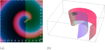
Figure 1: (a) Snapshot of spiral wave in the Barkley model (2) ($u$: red colour component, $v$: blue colour component), drifting in a stepwise inhomogeneity of paramer $c$ (green colour component), at base parameter values. The thin white line is the trace of the tip of the spiral, defined by $u(x,y,t)=u_{*}$, $v(x,y,t)=v_{*}$, in the course of a few preceding rotations. Yellow circles are positions of the centres calculated as period-averaged positions of the tip (Biktasheva et al., 2010). (b) Snapshot of scroll wave with buckled filament with negative tension in a thin layer of medium described by Barkley model (2) (Dierckx et al., 2012). Shown is the surface $u(x,y,z,t)=u_{*}$, coloured depending on $v$; the green line is the instant filament defined as the locus of $u(x,y,z,t)=u_{*}$, $v(x,y,z,t)=v_{*}$. The grayscale line on the top face is the trace of the upper end of the filament. Parameter values: in (a), $a=0.7$, $b=0.01$, $c=0.025$, $\delta c=0.001$,$D_{u}=1$, $D_{v}=0$, $u_{*}=0.5$, $v_{*}=0.34$, box size $24\times 24$; in (b), $a=1.1$, $b=0.19$, $c=0.02$, $D_{u}=1$, $D_{v}=0.1$, $u_{*}=0.5$, $v_{*}=0.36$, box size $20\times 20\times 6.9$.

Unlike the Wiener and Rosenblueth’s 2D theoretical abstraction, real excitable and oscillatory media, including BZ reaction and heart muscle, are three-dimensional (3D). Explicit experimental data on 3D extensions of spiral waves were first presented by Winfree (1973) in his variant of BZ reaction. He also coined the term “scroll waves” (see Figure 1(b)). While spiral waves rotate around their “cores”, which can be considered point-like geometric objects, scroll waves rotate around “filaments”, line-like geometric objects. Winfree also called them “organizing centres” (Winfree and Strogatz, 1983), but in a sense different from what it means for the social amoebae, as there are no living bodies to receive the signals in the BZ reaction. Rather, the filaments organize the waves in the sense that the wavefield in the whole volume follows what happens around the filament, and the rest of the wavefield can be more or less predicted using Huygens principle, as shown by Wiener and Rosenblueth.

As spiral and scroll waves do not require any obstacles to rotate about, they can be located anywhere within the reactive medium. An inevitable, even if not immediately evident, consequence of that is that their position can change in time, i.e. they can drift, as illustrated by Figure 1. Experimental and numerical studies of the drift have revealed that in many cases it is convenient to consider spiral waves as “particles”, interacting with each other or reacting to external perturbations as localized, point-wise objects, the location being at the core around which the spiral rotates. The scroll waves in 3D have more degrees of freedom: their filaments can not only move in space, but also change shape. The phase of rotation may vary along the filament, the feature known as “twist” of the scroll wave. Twist of a scroll wave and curvature of its filament are specifically three-dimensional factors of its dynamics.

It also turned out that not only it is convenient to describe motion of spirals and scrolls in terms of their cores and filaments, but it is possible to predict their motion in terms of cores and filaments coordinates only (particularly considering the phase as one of the coordinates). In this review, we aim to briefly discuss why this approach works and what sort of results it can produce. The literature on scroll dynamics is vast and the available space enforce us to restrict to selected examples in the narrow topic defined by the title of this chapter. We shall neglect plenty of other interesting results, including most of twist-related effects and everything related to competition and meander.

2 Wave-particle duality of spiral waves

The possibility to replace consideration of spiral waves by “particles”, interacting with each other or reacting to external perturbations, is in a seeming contradiction with the wave-nature of these objects. The spiral waves “look” like non-localized objects, filling up all available space, but “behave” like localized objects. The mathematical nature of this paradox was brought to the forefront by Biktasheva and Biktashev (2003) in terms of perturbative dynamics of spiral waves, i.e. drift of spirals in response to symmetry-breaking perturbations, such as spatial gradient of medium parameters or their resonant periodic modulation in time. Following (Biktashev and Holden, 1995), consider a reaction diffusion system

$$\partial_{t}\mathbf{u}=\mathbf{f}(\mathbf{u})+\mathbf{D}\nabla^{2}\mathbf{u}+\epsilon\mathbf{h},$$ (1)

where $\mathbf{u}=\mathbf{u}({\vec{r}},t)$, $\mathbf{f},\mathbf{h}\in\mathbb{R}^{\ell}$, $\mathbf{D}\in\mathbb{R}^{\ell\times\ell}$, $\ell\geq 2$, ${\vec{r}}\in\mathbb{R}^{2}$, with perturbation $\epsilon\mathbf{h}=\epsilon\mathbf{h}({\vec{r}},t,\mathbf{u},\nabla\mathbf{u},\dots)$, $||\epsilon\mathbf{h}||\ll 1$, and assume existence, at $\epsilon=0$, of stationary rotating spiral solutions

$$\mathbf{u}({\vec{r}},t)=\mathbf{U}(\rho({\vec{r}}-{\vec{R}}),\theta({\vec{r}}-{\vec{R}})+\omega t-\Phi)$$ (2)

where $\rho(),\theta()$ are polar coordinates centered at ${\vec{R}}$, constant $\omega$ is the angular velocity of spiral wave rotation, which up to the sign is uniquely defined by medium properties ($\mathbf{f}()$ and $\mathbf{D}$), and arbitrary constants ${\vec{R}}=(X,Y)$ and $\Phi$ are the location of the core of the spiral and its fiducial (initial) phase at $t=0$. Then the first order perturbation theory in $\epsilon$ gives solutions close to (2) with $R=X+iY$ and $\Phi$ slowly varying according to motion equations

$$\dot{R}=\epsilon H_{1}({\vec{R}},\Phi,t),\qquad\dot{\Phi}=\epsilon H_{0}({\vec{R}},\Phi,t).$$ (3)

The velocities of spatial drift, $H_{1}$, and temporal/phase drift, $H_{0}$, are linear functionals of the perturbation,

$$H_{n}=\oint_{t-\pi/\omega}^{t+\pi/\omega}\frac{\omega\,{\mathrm{d}}{t^{\prime}}}{2\pi}\iint\limits_{\mathbb{R}^{2}}{\mathrm{d}}^{2}{\vec{r}}\;e^{in(\Phi-\omega{t^{\prime}})}\left\langle\mathbf{W_{n}}(\rho,\theta+\omega{t^{\prime}}-\Phi)),\mathbf{h}\right\rangle,$$ (4)

where $\mathbf{h}$ is evaluated at the unperturbed solution (2).

Figure 2: Density plots of the components of the spiral wave solution and its response functions in the Oregonator model (2) for $\varepsilon=0.06$, $f=1.75$, $q=0.002$, $D_{u}=1$, $D_{v}=0.6$, the radius of the disk is 15 dimensionless units. In each plot, white corresponds to a value $A$ and black corresponds to $-A$ where $A$ is chosen individually for each plot, e.g. for the activator component of $\mathbf{U}$, $A=1.2$. The grey periphery of the plots in columns 2–4 corresponds to 0. The central areas are also shown magnified in the small corner panels.

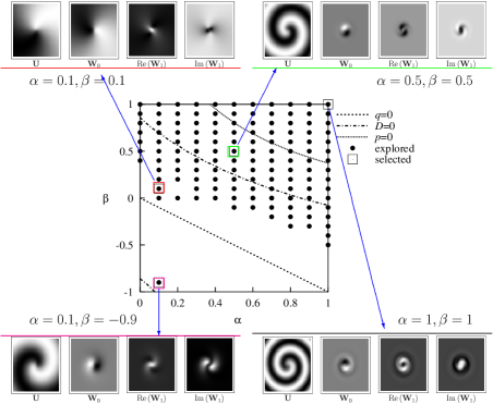
Figure 3: Density plots of the components of the spiral wave solution and its response functions in the complex Ginzburg-Landau equation (6), at various parameter values. In the legend: $p=2\left(\alpha\beta-1+k^{2}\left(3+2\beta^{2}-\alpha\beta\right)\right)/(1+\beta^{2})$, $q=-4k\left((\alpha+\beta)(1-k^{2})\right)(1+\beta^{2})$, $D=(p/3)^{3}+(q/2)^{2}$, and $k=k(\alpha,\beta)$ is the asymptotic wavenumber of the spiral (Biktasheva and Biktashev, 2001).

The kernels $\mathbf{W_{0,1}}$ of these functionals, which we call response functions (RFs), are critical eigenfunctions of the adjoint linearized problem. These eigenfunctions are dual to the eigenfunctions of the linearized problem produced by the generators of the Euclidean symmetry group, sometimes called Goldstone Modes (GMs). The “wave-particle’ duality then reduces to the difference between these eigenfunctions. The GMs, constructed from spatial derivatives of the spiral wave solution, are non-localized. The RFs, however, are essentially localized, i.e. exponentially decay far from the core of the spiral. This is of course only possible because the linearized problem is not self-adjoint.

The spiral waves have localized response functions in both excitable and oscillatory media. Figure 2 shows response functions in the two-component Oregonator (Tyson and Fife, 1980) model of the BZ reaction,

$$\partial_{t}u = \frac{1}{\varepsilon}\left(u(1-u)-fv\frac{u-q}{u+q}\right)+D_{u}\nabla^{2}u,$$

$$\partial_{t}v = u-v+D_{v}\nabla^{2}b,$$ (5)

for a choice of parameters $\varepsilon,f,q$ that gives excitable dynamics. Figure 3 shows response functions in the complex Ginzburg-Landau equation (CGLE) (Kuramoto and Tsuzuki, 1975),

$$\partial_{t}w=w-(1-i\alpha)w|w|^{2}+(1+i\beta)\nabla^{2}w,\qquad w=u+iv\in\mathbb{C},$$ (6)

which is the “archetypical” oscillatory reaction-diffusion model, in the sense that it is a normal form of a reaction-diffusion system near a supercritical Hopf bifurcation in its reaction part. In CGLE, the response functions are localized for all sets of parameters where stable spiral wave solutions exist, with qualitative changes across critical lines in the parameter space (Biktasheva and Biktashev, 2001). Notice the non-monotonous behaviour (“halo”) in RFs close to the Eckhaus instability line (Figure 3, bottom right inset). This can have phenomenological implication for the dynamics of spirals and scrolls, discussed later.

Apparently, the defining condition for the RFs’ localization is the direction of the group velocity: a spiral wave will have localized RFs and behave as a localized object if and only if it is a source of waves, so that far from the core, the group velocity is directed outwards (Biktashev et al., 1994; Sandstede and Scheel, 2004).

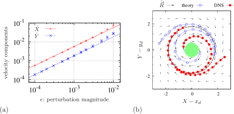
Figure 4: Drift of spiral waves: asymptotic theory vs direct numerical simulations. (a) The velocity of the drift caused by the gradient of parameter $a$ in the Barkley model (2), symbols for DNS and lines for the asymptotics, for base values of parameters $a=0.7$, $b=0.01$, $c=0.025$, $D_{u}=1$, $D_{v}=0$. (b) The trajectories of the drift caused by a disk-shaped inhomogeneity in parameter $\gamma$ in the FitzHugh-Nagumo model (2), at base values $\alpha=0.3$, $\beta=0.68$, $\gamma=0.5$, $D_{u}=1$, $D_{v}=0$. The small arrows indicate drift velocities as predicted by the asymptotic theory, and the filled and open circles show the instantaneous centers of rotation of the spiral wave, measured with the interval of one period of rotation. See (Biktashev et al., 2010; Biktasheva et al., 2010) for detail.

Figure 4 reproduces two selected results illustrating how well the perturbation theory works, for two classical simplified excitable media models, the FitzHugh-Nagumo model (Winfree, 1991a)

$$\partial_{t}u = \frac{1}{\alpha}\left(u-\frac{u^{3}}{3}-v\right)+D_{u}\nabla^{2}u,$$

$$\partial_{t}v = \alpha\left(u-\beta v+\gamma\right)+D_{v}\nabla^{2}v,$$ (7)

and Barkley model (Barkley, 1991)

$$\partial_{t}u = \frac{1}{c}u(1-u)\left(u-\frac{v-b}{a}\right)+D_{u}\nabla^{2}u,$$

$$\partial_{t}v = u-v+D_{v}\nabla^{2}v.$$ (8)

The trajectories in Figure 4(b) correspond to the case of the response function $\mathbf{W_{1}}$ with non-monotonic behaviour (the “halos” in Figure 3, bottom right, are an extreme case of such non-monotonic RFs). Here, small inhomogeneity attracts a spiral wave at larger distances and repels it at smaller distances. This alternating attraction/repulsion causes the spiral wave to “orbit” around at a certain stable distance, where the radial component of the “interaction force” vanishes.

There are important examples of spirals dynamics due to factors that are not small perturbations in the sense of (1), even though their action on the spirals is small. These include interaction of spiral waves with boundaries, and their interaction with each other (which may be considered as interaction of each spiral with the boundary between their “domains of influence”). These interactions are weak when the distance from the spiral core to the boundary or between the spiral cores is large. The mathematical aspects of particle-like behaviour in such cases are less clear. In the few examples where analytical answers are known, this seems to be associated with the exponential growth of solutions of the non-homogeneous linearized problem with the free term given by the spatial gradient of the spiral wave solution, see e.g. (Biktashev, 1989). This is also stipulated by the outward direction of the group velocity. Therefore both localization properties seem to be equivalent. That is, if a spiral wave does not feel a weak inhomogeneity when far from it, it will not feel a non-flux boundary at the same distance. Although this equivalence is quite plausible physically, mathematically it is still an open question.

3 Perturbative dynamics of scrolls, and tension of filaments

The perturbative dynamics of spiral waves can be extended to scroll waves. In 3D, there are interesting phenomena even in absence of any symmetry breaking perturbations. Following Keener (1988), consider a generic reaction-diffusion system (1) in ${\vec{r}}\in\mathbb{R}^{3}$ at $\mathbf{h}\equiv 0$, and assume, as before, existence of stationarily rotating spiral solutions (2) in $\mathbb{R}^{2}$. A simple extension of spiral wave solution to the third spatial dimension is called a straight scroll wave. More generically, a scroll wave solution in $\mathbb{R}^{3}$ may be viewed as a solution of the form

$$\mathbf{u}({\vec{R}}+{\vec{N}}\rho\cos\theta+{\vec{B}}\rho\sin\theta,t)=\mathbf{U}(\rho,\theta+\omega t-\Phi)+\mathcal{O}(\epsilon),$$ (9)

where $\epsilon$ is now a formal small parameter measuring deformation of a scroll wave compared to the straight scroll, ${\vec{R}}={\vec{R}}(\sigma,t)$ is the parametric equation of filament position at time $t$, $\Phi=\Phi(\sigma,t)$ is the rotational phase distribution, ${\vec{N}}={\vec{N}}(\sigma,t)$ and ${\vec{B}}={\vec{B}}(\sigma,t)$ are the unit principal normal and binormal vectors to the filament at point ${\vec{R}}(\sigma,t)$. Vectors ${\vec{N}}$ and ${\vec{B}}$ together with tangent vector ${\vec{T}}$ make a Frenet-Serret triple. In terms of the arclength differentiation operator $\mathcal{D}_{s}{u}(\sigma)=|\partial_{\sigma}{\vec{R}}|^{-1}\partial_{\sigma}u(\sigma)$, the tangent vector is ${\vec{T}}=\mathcal{D}_{s}{{\vec{R}}}$, the curvature $\kappa$ and the normal unit vector ${\vec{N}}$ are defined by $\kappa{\vec{N}}=\mathcal{D}_{s}{{\vec{T}}}$, and the binormal vector ${\vec{B}}={\vec{T}}\times{\vec{N}}$ completes the triad. The resulting filament’s equation of motion, at small filament curvature, $\kappa=\mathcal{O}(\epsilon)$, and small twist, $\mathcal{D}_{s}\Phi=\mathcal{O}(\epsilon)$, can be written as (Biktashev et al., 1994)

$$\partial_{t}{\vec{R}}=\gamma_{1}\mathcal{D}_{s}^{2}{\vec{R}}+\gamma_{2}\left[\mathcal{D}_{s}{\vec{R}}\times\mathcal{D}_{s}^{2}{\vec{R}}\right]+\mathcal{O}(\epsilon^{2}),$$ (10)

and it is decoupled from the evolution equation for the phase $\Phi(\sigma,t)$. Equation (10) is written in the assumption that parameter $\sigma$ of the filament is chosen in such a way that a point with a fixed $\sigma$ moves orthogonally to the filament (hence no component along ${\vec{T}}$).

The Frenet-Serret description is easy to understand but it has a significant disadvantage: it becomes degenerate at zero filament curvature, $\kappa=0$. An alternative description, free from this disadvantage, is in terms of Fermi-Walker coordinates, corresponding to a Levi-Civita (torsion-free metric) connection along the filament (hereafter called Fermi coordinates for brevity). This changes the scroll’s phase definition but does not affect (10) as it is decoupled.

The coefficients $\gamma_{1}$, $\gamma_{2}$ in (10) are calculated using the response functions $\mathbf{W_{1}}$ of the corresponding 2D spiral waves as

$$\gamma_{1}+i\gamma_{2}=-\frac{1}{2}\int\limits_{0}^{\infty}\oint\left[\mathbf{W_{1}}(\rho,\theta)\right]^{+}\mathbf{D}e^{-i\theta}\left(\partial_{\rho}-\frac{i}{\rho}\partial_{\theta}\right)\mathbf{U}(\rho,\theta)\;{\mathrm{d}}\theta\;\rho\,{\mathrm{d}}\rho.$$ (11)

Now let us consider the total length of the filament, defined at each $t$:

$$S(t)=\int{\mathrm{d}}{s}=\int\left|\partial_{\sigma}{\vec{R}}\right|\,{\mathrm{d}}\sigma.$$ (12)

Differentiation of (12), with account of (10) and using integration by parts, reveals that, neglecting boundary effects (absent for closed filaments and vanishing for smooth impermeable boundaries), the rate of change of the total length is

$$\dfrac{{\mathrm{d}}{S}}{{\mathrm{d}}{t}}=-\gamma_{1}\int\kappa^{2}\,{\mathrm{d}}{s}+\mathcal{O}(\epsilon^{2}).$$ (13)

This implies that, within the applicability of the perturbation theory, unless the filament is straight, the total length of the filament decreases if $\gamma_{1}>0$ and increases if $\gamma_{1}<0$. Hence the coefficient $\gamma_{1}$ was called “filament tension” in (Biktashev et al., 1994).

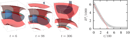
Figure 5: Dynamics of a quarter of a scroll ring in FitzHugh-Nagumo model (2), at $\alpha=0.30$, $\beta=0.71$, $\gamma=0.5$, $D_{u}=1$, $D_{v}=0$ (positive filament tension) in a box $33\times 33\times 40$ with periodic boundary conditions in the $z$ direction. The right panel shows evolution of the square of the radius of the instant scroll filament, defined as the locus $u=0$. Equation (10) predicts that the square of the period-average of the radius depends linearly on $t$, with the slope $-2\gamma_{1}$. The parameters for this example are taken from (Foulkes et al., 2010).

Filament tension can be found via the asymptotic rate of shrinkage or expansion of large scroll rings with exact axial symmetry (see Figure 5). This is only formally valid for scroll rings of sufficiently large radii in the unbounded space. Depending on the model, shrinkage of a scroll ring with positive filament tension may lead to its collapse, or may stop at some finite radius, while the ring continues to drift along its symmetry axis (Brazhnik et al., 1987; Skaggs et al., 1988), see Figure 5. Possible theoretical explanations of this may involve higher-order corrections to (10) and/or interaction of different pieces of the scroll ring with each other, in the same way as 2D spirals interact; which if either of these is the dominant reason in any particular case is, as far as we are aware, currently an open question. Apart from simple scroll rings, there are more complicated structures with twisted, linked and/or knotted filaments that can be persistent in some models, see (Winfree, 2001, pp.483–490) for the long story.

Filament tension depends on parameters of the medium, typically becoming negative in media with lower exitability, where spiral waves have larger cores (Panfilov and Rudenko, 1987). This can be substantiated by the “kinematic” theory of excitation waves (Brazhnik et al., 1987). However, there are exceptions to the rule: e.g. Alonso and Panfilov (2008) found an example where negative filament tension is observed at high excitability.

A simple but fundamental result is that when diffusivities of all the reagents are equal, $(\mathbf{D})_{ij}=D\delta_{ij}$, then $\gamma_{2}=0$ and $\gamma_{1}=D>0$ (Panfilov et al., 1986). A less trivial result is about filament tension in the CGLE (6), where it has been shown that $\gamma_{2}=0$, $\gamma_{1}=1+\beta^{2}>0$, see e.g. (Aranson and Kramer, 2002) for discussion and references. So in both these cases the filament tension is guaranteed to be positive. We do not know of any generic results about negative filament tension.

A higher-order asymptotic equation for filament motion was obtained by Dierckx and Verschelde (2013). Unlike the leading order (10), it is coupled to the evolution of the phase:

$$\partial_{t}\phi = a_{0}w^{2}+b_{0}\kappa^{2}+d_{0}\mathcal{D}_{s}w+\mathrm{h.o.t.},$$

$$\partial_{t}{\vec{R}} = (\gamma_{1}+a_{1}w^{2}+b_{1}\kappa^{2}+d_{1}\mathcal{D}_{s}w)\mathcal{D}_{s}^{2}{\vec{R}}$$ (14)

$$+(\gamma_{2}+a_{2}w^{2}+b_{2}\kappa^{2}+d_{2}\mathcal{D}_{s}w)\mathcal{D}_{s}^{\vec{R}}\times\mathcal{D}_{s}^{2}{\vec{R}}$$

$$+c_{1}w\mathcal{D}_{s}^{3}{\vec{R}}+c_{2}w\mathcal{D}_{s}{\vec{R}}\times\mathcal{D}_{s}^{3}{\vec{R}}$$

$$-e_{1}\mathcal{D}_{s}^{4}{\vec{R}}-e_{2}\mathcal{D}_{s}{\vec{R}}\times\mathcal{D}_{s}^{4}{\vec{R}}+\mathrm{h.o.t.},$$

where $\phi$ is the scroll phase measured in the Fermi frame, and $w$ is the corresponding twist, $w=\mathcal{D}_{s}\phi=\mathcal{D}_{s}\Phi-\tau$, where $\tau$ is the filament torsion, $\tau={\vec{B}}\cdot\mathcal{D}_{s}{\vec{N}}$. The vector-function ${\vec{R}}(s,t)$ in (3) is the “virtual filament” which has to be defined more precisely than (9), and the coefficients are defined as integrals involving spiral wave response functions, similar to but more complicated than (11); see (Dierckx and Verschelde, 2013) for detail.

4 Scroll wave turbulence

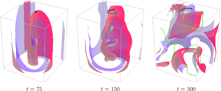
Figure 6: Negative filament tension instability causes scroll wave turbulence. Barkley model (2) with parameters $a=1.1$, $b=0.19$, $c=0.02$, $D_{u}=1$, $D_{v}=0$, box size $40\times 40\times 50$, instant filaments (green) defined as $u=v=0.5$. Wavefronts are cut out by clipping planes halfway through the volume, to reveal the filaments (Dierckx et al., 2012).

A negative filament tension implies that the straight scroll of a sufficient lentgh should be unstable. It was recognized rather early, that unless restabilized by some mechanism beyond (10), such instability can lead to complex spatio-temporal behaviour, possibly chaotic (Brazhnik et al., 1987; Biktashev et al., 1994). A particular interest for this complicated behaviour was due to its possible relation to cardiac fibrillation, with which it would have a number of phenomenological features in common (Biktashev et al., 1994; Winfree, 1994; Biktashev, 1998). The predicted “scroll wave turbulence” was confirmed by numerical simulations, first in the FitzHugh-Nagumo model (2) (Biktashev, 1998), and then in Barkley model (2) (Alonso et al., 2004), Oregonator model of the BZ reaction (2) (Alonso et al., 2006), and Luo-Rudy model of heart ventricular tissue (Alonso and Panfilov, 2007) to name a few; see (Alonso et al., 2013) for a recent review.

Based on the generic results mentioned above, chances to observe scroll wave turbulence mediated by negative filament tension in a BZ reaction should be higher when some of the reagents are immobilized, since scalar diffusivity matrix implies positive filament tension; in the excitable rather than oscillatory regime, since tension in the CGLE is always positive; and preferably in the “lower excitability” case. The latter prediction concurs with Oregonator simulations by Alonso et al. (2006).

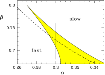
Figure 7: Part of the parameter space in the FitzHugh-Nagumo model (2), giving alternative spiral wave solutions, at fixed $\gamma=0.5$. The dashed line corresponds to zero tension. From Foulkes et al. (2010).

We mentioned earlier that the angular velocity $\omega$ of the spiral rotation is uniquely determined by the properties of the medium. This is not strictly true. Typically, there is a discrete set of possible $\omega$ values, and in some cases there may be more then one of them. Winfree (1991b) identified a set of parameters in the FitzHugh-Nagumo model (2), which could, depending on initial conditions, support two alternative spiral wave solutions with different $\omega$. Figure 7 shows a region in the parameter space with this property. Each of the alternative spiral waves is stable against small perturbations, but larger perturbations can convert one sort of spiral to the other. Foulkes et al. (2010) investigated such conversions and some implications for the dynamics of scroll waves in 3D. One nontrivial effect observed there is shown in Figure 8.

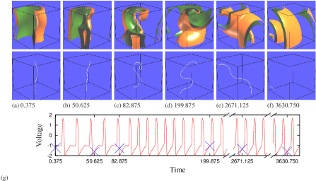
Figure 8: Evolution of a slow helical scroll with negative filament tension at $\alpha=0.3$, $\beta=0.71$, $\gamma=0.5$, $D_{u}=1$, $D_{v}=0$, box size $50\times 50\times 50$. (a-f) (Top) isosurfaces of the $u$-field; (middle) filament ($u=v=0$) only. (g) action potentials with blue crosses marking the times at which the snapshots were taken. The helix initially expands and turbulizes correspondingly to its negative tension, but then converts to its positive-tension alloform and contracts. From Foulkes et al. (2010).

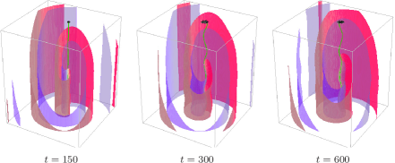
Figure 9: Short-wave filament instability causes restabilized “wrinkled” filament. Barkley model with parameters $a=0.66$, $b=0.01$, $c=0.025$, $D_{u}=1$, $D_{v}=0$, box size $40\times 40\times 50$, instant filaments (green) defined as $u=v=0.5$. Wavefronts are cut out by clipping planes (Dierckx et al., 2012).

In various models, the straight scrolls may become unstable through mechanisms different from the negative tension in (10). Henry and Hakim (2002) found that some parameter changes in Barkley model (2) can cause finite-wavelength instability of a scroll, while the filament tension remains positive. A different type of finite-wavelength instability at positive filament tension was found in CGLE by Aranson and Bishop (1997). They interpreted it in terms of “self-acceleration” of spiral waves, at parameter values where the dynamics of spiral waves in 2D is not well described by the perturbative dynamics (3) and further corrections are required. Interestingly, these two finite-wavelength instabilities have different outcomes: in CGLE, this leads to turbulent-like behaviour (Aranson and Bishop, 1997; Reid et al., 2011) visually similar to that shown in Figure 6, whereas in Barkley model, it leads to re-stabilized “wrinkled” or “zig-zag” shape of filaments, as shown in Figure 9 (Henry and Hakim, 2002; Dierckx et al., 2012). Clearly, a mere linearized theory can not describe the outcome of any such instability and more detailed study would be required to make any predictions there.

Finally, complex turbulent-like behaviour of scroll waves may be related to spatial heterogeneity. Among these, we mention the cases described by Fenton and Karma in models with spatially varying anisotropy, aimed at representing characteristic features of cardiac ventricular muscles,

$$\partial_{t}\mathbf{u}=\mathbf{f}(\mathbf{u})+\sum\limits_{i,j=1}^{3}\partial_{i}\left(D^{i,j}({\vec{r}})\partial_{j}\right)\mathbf{P}\mathbf{u},$$ (15)

where $\mathbf{P}\in\mathbb{R}^{\ell\times\ell}$ is a constant matrix representing relative diffusivities of the components  (Fenton and Karma, 1998a, b). Another often considered possibility is scroll turbulence due to purely 2D mechanisms which make spiral waves unstable, e.g. (Panfilov and Holden, 1990) and which of course reveal themselves in 3D as well (Clayton and Holden, 2003; Clayton et al., 2006; Clayton, 2008; Reid et al., 2011).

5 Rigidity of scroll filaments: pinning and buckling

The scroll wave turbulence mediated by negative filament tension is an essentially 3D phenomenon: it happens when spiral waves in a 2D medium with the same parameters are perfectly stable. So such turbulence is not observed in quasi-two-dimensional domains, say in thin layers of reactive medium. A gradual increase of the reactive layer thickness reveals that between the stable quasi-two-dimensional behaviour and the three dimensional turbulence, there are intermediate regimes, one of which is the “buckled filament” illustrated in Figure 1(b) for the Barkley model. Similar regimes were observed in simulations of Luo-Rudy cardiac model by Alonso and Panfilov (2007). A qualitative and quantitative explanation of such filament buckling proposed by Dierckx et al. (2012) was based on a simplified version of the higher-order motion equations (3). In particular, it gives the expression for the critical layer thickness, above which the buckling bifurcation happens, in the form $L_{*}=\pi|e_{1}/\gamma_{1}|^{1/2}$, where $e_{1}$ is the coefficient at the fourth arclength derivative in (3), and in this sense it is analogous to the rigidity of an elastic beam. So, within this mechanical analogy, the stability threshold for a straight scroll is determined by the interplay between filament tension $\gamma_{1}$ (negative of the “mechanical stress”) and the filament “rigidity” $e_{1}$, which is similar to the Euler’s buckling instability of a beam under a stress, hence the term “buckling” used to describe this deformation of the scrolls.

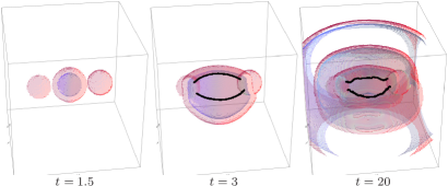
Figure 10: Schematic of the experiments done by Jiménez and Steinbock (2012). The upper half of a spherical wave is cut when it is passing through the beads thus forming two almost semi-circular filaments. The filaments become pinned to the beads and evolve to a stable configuration which depends on their tension, rigidity and interaction force between them. Oregonator model (2) with parameters $q=0.002$, $f=1.75$, $\varepsilon=0.06$, $D_{u}=D_{v}=0.5$, $u_{*}=0.24$, $v_{*}=0.075$, box size $50\times 50\times 50$. Wavefronts are cut out by clipping planes.

Experimental evidence of scroll filament rigidity was demonstrated in BZ reaction, with filaments pinned to inexcitable inclusions (Jiménez and Steinbock, 2012; Nakouzi et al., 2014), see Figure 10. In these experiments, the steady shapes of the filaments were determined, as well as their relaxation dynamics. The authors were able to describe the steady shapes using a variant of (3), with added phenomenological description of the interaction of filaments with each other. Fitting the theoretical curves to the experimentally found filament shapes allowed quantitative experimental measurement of the filament rigidity (Nakouzi et al., 2014).

6 Filament statics, geodesic principle and Snell’s law

For cardiac applications, anisotropy and inhomogeneity are very important. We have already mentioned above the instability and scroll turbulence related to inhomogeneous anistoropy. The “opposite” of scroll turbulence is the situation when scroll dynamics converges to a stable equilibrium position. For positive filament tension, in a spatially uniform, isotropic medium and when interaction with boundaries or other filaments can be neglected, the answer is straightforward: a straight filament, stretching in any direction. Motivated by numerical simulations of scroll waves in models with anisotropic diffusion such as (15), and by experiments with re-entrant excitation waves in cardiac tissue, Wellner et al. (2002) came up with a “geodesic hypothesis”: that for given positions of the filament end points (say if the filament is anchored to inexcitable inclusions), the steady scroll filament shape will be a geodesic in a metric related to the diffusivity tensor, $g_{ij}=(D^{-1})_{ij}$. For instance, in a cardiac muscle, the preferrable orientation of a scroll filament would be along the fibers, i.e. direction of the maximal diffusivity of the transmembrane potential. As ten Tusscher and Panfilov (2004) noted, the metric defining the steady-state geometries of filaments, can be conveniently formulated in terms of excitation wave propagation time: given its end points, the filament will follow the quickest path connecting the end points. This hypothesis was confirmed by Verschelde et al. (2007) who generalized the equation (10) for the anisotropic media, under the assumption of $\det(D^{ij})=\mathrm{const}$. An empirical generalization of this geodesic principle for non-uniform $\det(D^{ij})$, based on simulations using Barkley model, was suggested by Wellner et al. (2010), in the form $g_{ij}=\det(D^{ij})(D^{-1})_{ij}$. An interesting study has been performed by Zemlin et al. (2014), who investigated in numerical simulations the analogue of “Snell’s law”for a filament crossing a boundary between media with different diffusivities, following from the geodesic principle, and the limits of its applicability.

References

- Alcantara and Monk [1974] F. Alcantara and M. Monk. Signal propagation during aggregation in the slime mould Dictyostelium discoideum. J. gen. Microbiol., 85:321–334, 1974.
- Alonso and Panfilov [2007] S. Alonso and A. V. Panfilov. Negative filament tension in the Luo-Rudy model of cardiac tissue. Chaos, 17:015102, 2007.
- Alonso and Panfilov [2008] S. Alonso and A. V. Panfilov. Negative filament tension at high excitability in a model of cardiac tissue. Phys. Rev. Lett., 100:218101, 2008.
- Alonso et al. [2004] S. Alonso, R. Kahler, A. S. Mikhailov, and F. Sagues. Expanding scroll rings and negative tension turbulence in a model of excitable media. Phys. Rev. E, 70:056201, 2004.
- Alonso et al. [2006] S. Alonso, F. Sagues, and A. S. Mikhailov. Negative-tension instability of scroll waves and Winfree turbulence in the Oregonator model. Journal of Physical Chemistry A, 110:12063–12071, 2006.
- Alonso et al. [2013] S. Alonso, M. Bär, and A. V. Panfilov. Negative tension of scroll wave filaments and turbulence in three-dimensional excitable media and application in cardiac dynamics. Bull. Math. Biol., pages 1351–1376, 2013.
- Aranson and Bishop [1997] I. S. Aranson and A. R. Bishop. Instability and stretching of vortex lines in the three-dimensional complex Ginzburg-Landau equation. Phys. Rev. Lett., 79:4174–4177, 1997.
- Aranson and Kramer [2002] I. S. Aranson and L. Kramer. The world of the complex Ginzburg-Landau equation. Rev. Mod. Phys., 74:99–143, 2002.
- Balakhovskii [1965] I. S. Balakhovskii. Some regimes of excitation movement in ideal excitable tissue. Biofizika, 10:1063–1067, 1965. in Russian.
- Barkley [1991] D. Barkley. A model for fast computer simulation of waves in excitable media. Physica D, 49:61–70, 1991.
- Belousov [1959] B. P. Belousov. A periodic reaction and its mechanism. In Sbornik referatov po radiatsionnoj medicine za 1958, pages 145–147. Medgiz, Moscow, 1959. in Russian. See also in R. J. Field and M. Burger (eds.), Oscillations and traveling waves in chemical systems (Wiley, New York).
- Biktashev [1989] V. N. Biktashev. Drift of a reverberator in an active medium due to interaction with boundaries. In A. V. Gaponov-Grekhov, M. I. Rabinovich, and J. Engelbrecht, editors, Nonlinear Waves II. Dynamics and Evolution, pages 87–96. Springer, Berlin, 1989.
- Biktashev [1998] V. N. Biktashev. A three-dimensional autowave turbulence. Int. J. of Bifurcation and Chaos, 8:677–684, 1998.
- Biktashev and Holden [1995] V. N. Biktashev and A. V. Holden. Resonant drift of autowave vortices in 2d and the effects of boundaries and inhomogeneities. Chaos Solitons & Fractals, 5(3,4):575–622, 1995.
- Biktashev et al. [1994] V. N. Biktashev, A. V. Holden, and H. Zhang. Tension of organizing filaments of scroll wave. Phil. Trans. Roy. Soc. Lond. ser. A, 347:611–630, 1994.
- Biktashev et al. [2010] V. N. Biktashev, D. Barkley, and I.V. Biktasheva. Orbital motion of spiral waves in excitable media. Phys. Rev. Lett., 104:058302, 2010.
- Biktasheva and Biktashev [2001] I. V. Biktasheva and V. N. Biktashev. Response functions of spiral wave solutions of the complex Ginzburg-Landau equation. J. Nonlin. Math. Phys., 8 Supp.:28–34, 2001.
- Biktasheva and Biktashev [2003] I. V. Biktasheva and V. N. Biktashev. On a wave-particle dualism of spiral waves dynamics. Phys. Rev. E, 67:026221, 2003.
- Biktasheva et al. [2010] I. V. Biktasheva, D. Barkley, V. N. Biktashev, and A. J. Foulkes. Computation of the drift velocity of spiral waves using response functions. Phys. Rev. E, 81:066202, 2010.
- Brazhnik et al. [1987] P. K. Brazhnik, V. A. Davydov, V. S. Zykov, and A. S. Mikhailov. Vortex rings in excitable media. Zh. Eksp. Teor. Fiz., 93:1725–1736, 1987.
- Clayton [2008] R. H. Clayton. Vortex filament dynamics in computational models of ventricular fibrillation in the heart. Chaos, 18:043127, 2008.
- Clayton and Holden [2003] R. H. Clayton and A. V. Holden. Dynamics and interaction of filaments during reentry and fibrillation in mammalian virtual ventricular tissue. Int. J. of Bifurcation and Chaos, 13:3733–3745, 2003.
- Clayton et al. [2006] R. H. Clayton, E. A. Zhuchkova, and A. V. Panfilov. Phase singularities and filaments: Simplifying complexity in computational models of ventricular fibrillation. Prog. Biophys. Mol. Biol., 90:378–398, 2006.
- Dierckx and Verschelde [2013] H. Dierckx and H. Verschelde. Effective dynamics of twisted and curved scroll waves using virtual filaments. Phys. Rev. E, 88:062907, 2013.
- Dierckx et al. [2012] H. Dierckx, H. Verschelde, Ö. Selsil, and V. N. Biktashev. Buckling of scroll waves. Phys. Rev. Lett., 109:174102, 2012.
- Fenton and Karma [1998a] F. Fenton and A. Karma. Fiber-rotation-induced vortex turbulence in thick myocardium. Phys. Rev. Lett., 81:481–484, 1998a.
- Fenton and Karma [1998b] F. Fenton and A. Karma. Vortex dynamics in three-dimensional continuous myocardium with fiber rotation: Filament instability and fibrillation. Chaos, 8:20–47, 1998b.
- Foulkes et al. [2010] A. J. Foulkes, D. Barkley, V. N. Biktashev, and I. V. Biktasheva. Alternative stable scroll waves and conversion of autowave turbulence. Chaos, 20:043136, 2010.
- Henry and Hakim [2002] H. Henry and V. Hakim. Scroll waves in isotropic excitable media: Linear instabilities, bifurcations and restabilized states. Phys. Rev. E, 65:046235, 2002.
- Jiménez and Steinbock [2012] Z. A. Jiménez and O. Steinbock. Stationary vortex loops induced by filament interaction and local pinning in a chemical reaction-diffusion system. Phys. Rev. Lett., 109:098301, 2012.
- Keener [1988] J. P. Keener. The dynamics of 3-dimensional scroll waves in excitable media. Physica D, 31:269–276, 1988.
- Kuramoto and Tsuzuki [1975] Y. Kuramoto and T. Tsuzuki. Formation of dissipative structures in reaction-diffusion systems — reductive perturbation approach. Prog. Theor. Phys., 54:687–699, 1975.
- Nakouzi et al. [2014] E. Nakouzi, Z. Jiménez, V. N. Biktashev, and O. Steinbock. Analysis of anchor-size effects on pinned scroll waves and measurement of filament rigidity. to be published, 2014.
- Panfilov and Holden [1990] A. V. Panfilov and A. V. Holden. Self-generation of turbulent vortices in a two-dimensional model of cardiac tissue. Phys. Lett. A, 151:23–26, 1990.
- Panfilov and Rudenko [1987] A. V. Panfilov and A. N. Rudenko. Two regimes of the scroll ring drift in the three-dimensional active media. Physica, 28D:215–218, 1987.
- Panfilov et al. [1986] A. V. Panfilov, A. N. Rudenko, and V. I. Krinsky. Turbulent rings in three-dimensional active media with diffusion by two components. Biofizika, 31:850–854, 1986.
- Reid et al. [2011] J. C. Reid, H. Chaté, and J. Davidsen. Filament turbulence in oscillatory media. EPL, 94:68003, 2011.
- Sandstede and Scheel [2004] B. Sandstede and A. Scheel. Defects in oscillatory media: Toward a classification. SIAM J. Appl. Dyn. Syst., 3(1):1–68, 2004.
- Skaggs et al. [1988] W. Skaggs, E. Lugosi, and A. T. Winfree. Stable vortex rings of excitation in neuroelectric media. IEEE Transactions on Circuits and Systems, 35:784–787, 1988.
- ten Tusscher and Panfilov [2004] K. H. W. J. ten Tusscher and A. V. Panfilov. Eikonal formulation of the minimal principle for scroll wave filaments. Phys. Rev. Lett., 93:108106, 2004.
- Tyson and Fife [1980] J. J. Tyson and P. C. Fife. Target patterns in a realistic model of the Belousov-Zhabotinskii reaction. J. Chem. Phys., 73:2224–2237, 1980.
- Tyson and Murray [1989] J. J. Tyson and J. D. Murray. Cyclic AMP waves during aggregation of Dictyostelium amoeba. Development, 106:421–426, 1989.
- Verschelde et al. [2007] H. Verschelde, H. Dierckx, and O. Bernus. Covariant stringlike dynamics of scroll wave filaments in anisotropic cardiac tissu. Phys. Rev. Lett., 99:168104, 2007.
- Wellner et al. [2002] M. Wellner, O. Berenfeld, J. Jalife, and A. M. Pertsov. Minimal principle for rotor filaments. Proc. Natl. Acad. Sci. USA, 99:8015–8018, 2002.
- Wellner et al. [2010] M. Wellner, C. W. Zemlin, and A. M. Pertsov. Frustrated drift of an anchored scroll-wave filament and the geodesic principle. Phys. Rev. E, 82:036122, 2010.
- Wiener and Rosenblueth [1946] N Wiener and A. Rosenblueth. The mathematical formulation of the problem of conduction of impulses in a network of connected excitable elements, specifically in cardiac muscle. Archivos del Instituto de Cardiologia de Mexico, 16:205–265, 1946.
- Winfree [1972] A. T. Winfree. Spiral waves of chemical activity. Science, 175:634–636, 1972.
- Winfree [1973] A. T. Winfree. Scroll-shaped waves of chemical activity in 3 dimensions. Science, 181:937–939, 1973.
- Winfree [1991a] A. T. Winfree. Varieties of spiral wave behaviour: An experimentalist’s approach to the theory of excitable media. Chaos, 1:303–334, 1991a.
- Winfree [1991b] A. T. Winfree. Alternative stable rotors in an excitable medium. Physica D, 49(1):125 – 140, 1991b.
- Winfree [1994] A. T. Winfree. Electrical turbulence in three-dimensional heart muscle. Science, 266:1003–1006, 1994.
- Winfree [2001] A. T. Winfree. The Geometry of Biological Time. Second edition. Springer, USA, 2001.
- Winfree and Strogatz [1983] A. T. Winfree and S. H. Strogatz. Singular filaments organize chemical waves in three dimensions. Physica, 8D:35–49, 1983. 9D, pp. 65–80, 333–345 (1983), 13D, pp. 221–233 (1984).
- Zemlin et al. [2014] C. W. Zemlin, F. Varghese, M. Wellner, and A. M. Pertsov. Snell’s law and the validity of minimal principle for scroll wave filaments. to be published, 2014.
- Zhabotinsky [1964a] A. M. Zhabotinsky. Periodical oxidation of malonic acid in solution (a study of the Belousov reaction kinetics). Biofizika, 9:306–311, 1964a.
- Zhabotinsky [1964b] A. M. Zhabotinsky. Periodic liquid phase reactions. Proc. Ac. Sci. USSR, 157:392–95, 1964b.
- Zhabotinsky and Zaikin [1971] A. M. Zhabotinsky and A. N. Zaikin. Spatial phenomena in the auto-oscillatory system. In E. E. Selkov, A. A. Zhabotinsky, and S. E. Shnol, editors, Oscillatory processes in biological and chemical systems, page 279. Nauka, Pushchino, 1971.