Localized modes in two-dimensional Schrödinger lattices with a pair of nonlinear sites

Abstract

We address the existence and stability of localized modes in the two-dimensional (2D) linear Schrödinger lattice with two symmetric nonlinear sites embedded into it, and a generalization for moderately localized nonlinearity featuring two distinct symmetric maxima. The latter setting admits a much greater variety of localized modes. Symmetric, antisymmetric, and asymmetric discrete solitons are found, and a subcritical bifurcation, accounting for the spontaneous symmetry breaking (SSB) of the symmetric modes and transition to asymmetric ones, is identified. Existence and stability of more complex 2D solutions in the form of discrete symmetric and asymmetric vortices are also discussed.

1 Introduction

Discrete nonlinear systems, alias dynamical lattices, appear as basic models in various fields of physics. Fundamental excitations supported by the nonlinear lattice systems appear in the form of discrete solitons. In particular, such solitons can be investigated in the framework of the ubiquitous model based on the discrete nonlinear Schrödinger (DNLS) equation with the onsite cubic nonlinearity, or systems of such coupled equations [1]. Actually, the simplest variety of the DNLS equation is the one with a pair of nonlinear sites embedded into the host linear lattice [2, 3], and similar models with a pair of nonlinear sites side-coupled to a linear lattice [4].

It is well known that DNLS models of various types can be realized in optics, in the form of transversely coupled arrays of parallel nonlinear waveguides for optical [5] and plasmonic [6] waves. On the other hand, the DNLS equation is a standard mean-field model for Bose-Einstein condensates (BECs) trapped in deep periodic potentials created, as optical lattices, by the interference of laser beams illuminating the condensate in opposite directions, see original papers which elaborated this setting for the atomic condensates [7], and reviews [8]. In particular, new techniques for engineering various settings based on optical lattices have been developed recently [9]. Further, the DNLS model with a few nonlinear sites immersed into the linear host lattice can also be implemented in optics, by embedding nonlinear cores into the linear waveguiding array, as discussed in Ref. [10], and in BEC, by means of the Feshbach resonance [11], which can be induced locally by an external field in the condensate trapped in the optical lattice. The latter possibility was considered theoretically in various settings [12], and demonstrated experimentally in the ytterbium condensate, using an appropriate laser field [13].

One of fundamental dynamical effects featured by nonlinear lattices is spontaneous symmetry breaking (SSB). A typical manifestation of the SSB is the transition from symmetric to asymmetric discrete solitons in the system of two parallel DNLS chains, with the transverse linear coupling applied uniformly [14] or at single pair of sites [15]. The corresponding bifurcation, i.e., the destabilization of the symmetric solitons and emergence of asymmetric ones, is of the subcritical and supercritical types in the former and latter cases, respectively (the subcritical bifurcation, alias the phase transition of the first kind, generates pairs of stable and unstable asymmetric states prior to the destabilization of the parent symmetric one at the respective critical point [16]; the supercritical bifurcation is a manifestation of the phase transition of the second kind). Antisymmetric discrete solitons also exist in these systems, but they do not undergo the bifurcation.

Another setting, which makes it possible to study the SSB of discrete solitons in a single chain, is offered by the above-mentioned systems, based on the linear chain with two nonlinear sites embedded into [3] or side-coupled [4] onto it. In such models, the results can be obtained in an analytical form. Also recently considered was the linear chain with a pair of embedded sites with the quadratic (second-harmonic-generating), rather than cubic, nonlinearity [17], where analytical results can be obtained too.

In addition to the discrete systems, it is also possible to study solitons and their SSB phenomenology in semi-discrete settings, with a pair of localized elements, carrying the cubic [18] or quadratic [19] nonlinearity, which are embedded into a continuous linear medium. The latter setting may also be realized in both optics and BEC. A two-dimensional (2D) version of this setting, with the cubic nonlinearity concentrated at two separate spots, was recently considered too [20]. Generally speaking, discrete and continuous settings with a few localized nonlinear spots, or periodic arrays of such spots, belong to the vast realm of nonlinear lattices [21].

The subject of the present work is the study of 2D discrete solitons supported by the nonlinearity concentrated at or around two sites embedded into a host linear lattice, and the SSB phenomenology for such solitons. The basic model where this setting can be implemented is the 2D DNLS network with a pair of built-in nonlinear sites, or, in a more general form, with localized nonlinearity that has maxima at two distinct sites. This setting may be considered as a 2D version of the system introduced in Ref. [3]. It can be realized straightforwardly in BEC, using a deep optical lattice and the locally concentrated action of the Feshbach resonance, as mentioned above. In optics, the same setting may be built in the form of 2D waveguiding arrays written as a permanent structure in bulk materials [22], with the strong nonlinearity in selected cores created by means of dopants [23]. Alternatively, the effective nonlinearity of particular cores in the waveguiding array can be enhanced simply be making the effective cross-section area of this core smaller.

The model is formulated in Section II. Unlike its 1D counterpart the 2D model, even in the case of the single nonlinear core, does not admit analytical solutions. However, it gives rise to a much richer variety of localized modes and transformations between them than was previously found in the 1D geometry [3]. Results of the numerical analysis are reported in Sections III and IV for the cases of the strong and moderate localization of the nonlinearity, respectively. In particular, the SSB occurs, in contrast to the 1D system, for very broad solitons, and the character of the bifurcation is always strongly subcritical. The paper is concluded by Section IV.

2 The model

We consider the 2D DNLS equation as the model for the light transmission in the square-shaped array of coupled optical waveguides, with propagation distance $z$:

$$i\frac{du_{m,n}}{dz}+\Delta_{m,n}u_{m,n}+W_{m_{0},n_{0}}(l)|u_{m,n}|^{2}u_{m,n}=0,$$ (1)

where the discrete 2D Laplacian is $\Delta_{m,n}u_{m,n}=u_{m+1,n}+u_{m-1,n}+u_{m,n+1}+u_{m,n-1}-4u_{m,n}$. Two nonlinear sites, embedded into the host linear lattice along the horizontal direction, correspond to the following form of the local nonlinearity strength in Eq. (1):

$$W_{m_{0},n_{0}}(l)=\delta_{m_{0},n_{0}}+\delta_{m_{0}-l,n_{0}},$$ (2)

where $(m_{0},n_{0})$ and $l$ are integer which define the coordinates of the nonlinear cites and the distance between them.

It is also possible to consider two nonlinear sites embedded along the diagonal direction, i.e., $W_{m_{0},n_{0}}(l)=\delta_{m_{0},n_{0}}+\delta_{m_{0}-l,n_{0}-l}$. Below, we concentrate on the horizontal pair, as the diagonal one yields similar results, but with a weaker interaction between the nonlinear sites.

Stationary solutions to Eq. (1) with propagation constant $\omega$ are sought for as $u_{m,n}(z)=e^{i\omega z}U_{m,n}$, where stationary field $U_{m,n}$ (which is real for fundamental solitons, and complex for vortices) obeys equation

$$\omega U_{m,n}=\Delta_{m,n}U_{m,n}+W_{m_{0},n_{0}}(l)|U_{n}|^{2}U_{n}.$$ (3)

Stationary solutions are characterized by their norm (i.e., total power in the case of the array of optical waveguides),

$$N=\sum_{m,n=-\infty}^{+\infty}|U_{m,n}|^{2}.$$ (4)

As a generalization of the model with the two-site structure (2), we will also consider the one with the Gaussian profile of the localized double-spot nonlinearity,

$$\delta_{m_{0},n_{0}}\rightarrow\exp\left(-\frac{(m-m_{0})^{2}+(n-n_{0})^{2}}{(\Delta W)^{2}}\right),$$ (5)

in which the strong and moderate localization correspond, respectively, to $\Delta W\ll 1$ and $\Delta W\gtrsim 1$, as shown in Fig. 1. In the experiment, the Gaussian nonlinearity-modulation profile (5) may be realized by means of the respective distribution of the density of the resonant nonlinearity- inducing dopant, or by fabricating the array with the corresponding distribution of the cores’ effective cross-section area.

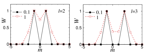
Figure 1: (Color online) The cross section of the nonlinearity-modulation profile, $W_{m,n=0}$, for the cases of strong ($\Delta W=0.1$) and moderate ($\Delta W=1$) localization [see Eq. (5)], and two values of the integer distance between the nonlinear sites, $l=2$ and $3$.

3 Modes supported by the strong localization of the nonlinearity ($\Delta W=0.1$)

Unlike its 1D counterpart, the present model, even in its simplest form, with a single or two nonlinear sites embedded into the linear host medium [see Eq. (2)], does not admit an analytical solution for stationary modes. Therefore, the starting point of the analysis is the anticontinuum limit (ACL) [1], which corresponds, in the present notation, to $\omega\rightarrow\infty$. In this limit, all the modes are built as configurations with nonzero amplitudes set only at sites carrying the strong nonlinearity. Such modes of the symmetric, asymmetric and antisymmetric types are schematically shown in Fig. 2, for $l=2$ and $l=3$.

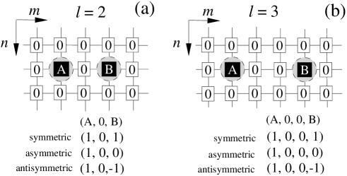
Figure 2: Top row is schematic distribution of exited sites in the 2D lattice. Gray circles show schematic localization of nonlinear spots. A and B stand for amplitudes at the nonlinear spots. In the bottom the modes of symmetric, asymmetric, and antisymmetric types are schematically shown in the anticontinuum limit; they are localized on two nonlinear sites separated by distance $l=2$ or $3$.

In the following, various modes are designated according to the ACL seeds from which they stem. The curves which represent the so found symmetric, asymmetric and antisymmetric modes by means of dependencies $N(\omega)$ are shown in Fig. 3. In contrast to the 1D model [3] and 2D continuous NLS model with periodic potential [24, 25], the norm of the localized modes diverges close to the phonon band, where the modes undergo delocalization, i.e., may be considered in the continuum approximation, with the nonlinear term multiplied by the $\delta$-function of the spatial coordinates. The continual 1D Schrödinger equation with such a nonlinear term gives rise to a family of solitons with a finite norm [18], while such solutions do not exist in the 2D case, which explains the above-mentioned divergence.

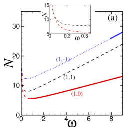
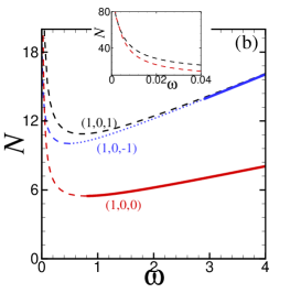
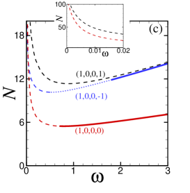
Figure 3: (Color online) Curves $N(\omega)$, the total power (norm) versus the propagation constant [see Eq. (4)], for families of symmetric (black), asymmetric (red) and antisymmetric (blue) modes. (a), (b) and (c) correspond to distances $l=1,2$ and $3$ between the strongly localized nonlinear sites, with $\Delta W=0.1$. Here and in similar figures following below, solid, dotted and dashed lines represent stable, oscillatory-unstable and strongly unstable branches of the solutions, respectively. Insets zoom areas in which the SSB bifurcation occurs.

At $l=1$, i.e., in the 2D linear host lattice with the adjacent pair of embedded nonlinear sites, the SSB, which gives rise to asymmetric localized mode ($1,0$) from the symmetric one ($1,1$), occurs in strongly delocalized states with large norms [see Fig. 3(a)]. The respective bifurcation is subcritical, hence the emerging branch of the asymmetric discrete solitons is unstable. With the decrease of $N$, it attains a turning point, corresponding to a minimum of $N$, at which the branch becomes stable. The stabilization of the asymmetric branch at the turning point, where it changes the sign of the slope, from $dN/d\omega<0$ to $dN/d\omega>0$, exactly agrees with the Vakhitov-Kolokolov (VK) criterion [26].

Increasing distance $l$ between the embedded nonlinear sites from $1$ to $3$, we observe that the SSB takes place for the modes which are so broad that they cannot be fitted to the computation domain. For the sake of the comparison with the 1D model [3], it is relevant to mention that the latter one also gives rise to the subcritical SSB bifurcation for $l\geq 2$, while, just for $l=1$, the respective bifurcation is supercritical in the 1D system [17], on the contrary to the results reported here. The difference in the character of the bifurcation (super/sub-critical) between the 1D and 2D settings with $l=1$ may be explained by the general trend of the SSB bifurcations to switch to the subcritical type with the increase of the dimension (for instance, the bifurcation driven by the cubic term is always supercritical in the zero-dimensional model, but tends to become subcritical in 1D). For the model with exactly two nonlinear sites, i.e., $\Delta W=0$, which corresponds to Eq. (2), the situation is virtually the same as displayed here for $\Delta W=0.1$.

The stability of the modes along solution branches has been checked through the computation of stability eigenvalues for small perturbations. The perturbed solution was looked as

$$u_{m,n}(z)=\left[U_{m,n}^{(s)}+a_{m,n}(z)\right]e^{i\omega z},$$ (6)

where $a_{m,n}(z)=p_{m,n}e^{i\lambda z}+q_{m,n}^{\ast}e^{-i\lambda^{\ast}z}$ is an eigenmode of small perturbations with (generally, complex) eigenvalue $\lambda$, added to stationary solution $U_{m,n}^{(s)}$ (the asterisk stands for the complex conjugate). Substituting expression (6) into Eq. (1) leads to the linearized eigenvalue problem, that can be written in the following matrix form,

$$\left(\begin{array}[]{cc}\hat{L}_{m,n}-\lambda&\hat{L}_{m,n}^{\prime}\\ -(\hat{L}_{m,n}^{\prime})^{\ast}&-\hat{L}_{m,n}-\lambda\end{array}\right)\left(\begin{array}[]{c}p\\ q\end{array}\right)=0$$ (7)

where operators are $\hat{L}_{m,n}=-\omega+\Delta_{m,n}+2W_{m,n}|U_{m,n}^{(s)}|^{2}$ and $\hat{L}_{m,n}^{\prime}=W_{m,n}\left(U_{m,n}^{(s)}\right)^{2}$. The stability of the solutions was then analyzed through the calculation of eigenvalues of Eq. (7), and verified by direct simulations of the perturbed evolution.

In this way, it was found that unstable modes designated in Fig. 3 may feature different types of the instability. In particular, as concerns the symmetric and antisymmetric modes shown in Fig. 3, the analysis demonstrates that the symmetric mode is strongly unstable due to the presence of purely imaginary eigenvalues, irrespective of the compliance with the VK criterion (recall that it gives only a necessary but not sufficient stability condition). On the other hand, the antisymmetric mode of the ($1,-1$) type, which is unstable at small $\omega$ to oscillatory perturbations, corresponding to a pair of complex eigenvalues, transforms into an oscillatory unstable state after the turning point. Then, it becomes stable at some critical propagation constant, whose value decreases with the increasing of distance $l$ between the nonlinear sites. This difference is also visible in the dynamical evolution of the corresponding modes, with the strong instability of mode ($1,1$) developing much faster than in the oscillatory instability of mode ($1,-1$) (not shown here in detail).

The SSB is characterized by the asymmetry parameter, which is defined as

$$\Theta\equiv\frac{U_{m_{0},n_{0}}^{2}-U_{m_{0}-l,n_{0}}^{2}}{U_{m_{0},n_{0}}^{2}+U_{m_{0}-l,n_{0}}^{2}},$$ (8)

and may be displayed as a function of $\omega$ or $N$. The respective results for strongly localized nonlinearity and for different distances between the nonlinear sites are presented in Fig. 4. It is seen that the SSB is strongly subcritical, with the unstable branches of the asymmetric modes going a long way in the direction of decreasing $N$, and only afterwards the branches turn back, recovering the stability of extremely asymmetric modes, with values of $\Theta$ very close to $1$.

Figure 4: Asymmetry parameter (8) of the mode (1,0), as a function of $\omega$ in (a), (c) and (e), and as a function of $N$ in (b), (d) and (f), for different distances between the nonlinear sites (indicated in each plot) in the case of the strong localization of the nonlinearity, $\Delta W=0.1$, for the same solutions which are shown in Fig. 3.

Dynamical properties of the localized modes are further illustrated by Fig. 5, which displays typical initial and final profiles, at $t=0$ and $t=20$, respectively, of symmetric, asymmetric and antisymmetric localized solutions, as well as the evolution of the initially excited sites. The figure also demonstrates that, at relatively large values of $\omega$, at which the asymmetric modes are strongly localized and stable, their symmetric and antisymmetric counterparts are unstable against symmetry- (or antisymmetry-) breaking perturbations, spontaneously transforming into the asymmetric mode. On the other hand, at small $\omega$, which implies that the discrete solitons are broad, they are unstable against full delocalization, as shown in the right-hand side of Fig. 5.

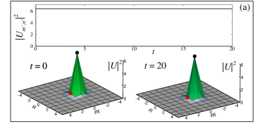
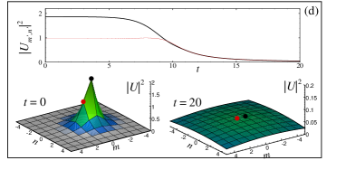
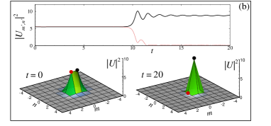
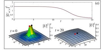
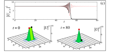
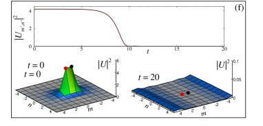
Figure 5: (Color online) The evolution of asymmetric [(a), (d)], symmetric [(b), (e)] and antisymmetric [(c), (f)] localized modes with $l=1$. In each subplot the dynamics of two initially excited sites $|U_{m^{\prime},n^{\prime}}|$, indicated by black and red dots on the initial ($t=0$) and final ($t=20$) profiles, is shown. The left column corresponds to $\omega=3$, and the right one to $\omega=0.1$. The only stablemode is the asymmetric one shown in (a) at $\omega=3$, the other examples being unstable.

4 Modes supported by the moderately localized nonlinearity ($\Delta W=1$)

The increase of the area of the nonlinearity localization, i.e., the increase of $\Delta W$ in Eq. (5), makes it possible to build a larger variety of 2D localized modes in the ACL, as shown in Figs. 6 and 7. In this section we study modes for $\Delta W=1$. For example, in the case of $l=2$ the system supports a mode of type ($0,1,0$), which does not exist in the limit of the strong localization. This is possible because in the ACL the amplitude at each site is related to the propagation constant and the magnitude of the nonlinear coefficient as follows: $U_{n}=\{\pm\sqrt{\omega/W_{n}},0\}$. In the case of the strong localization of $W_{n}$, one can construct only ACL modes localized on each of the nonlinear sites. On the other hand, with moderate localization of the nonlinearity, as in the case of $\Delta W=1$, it is possible to excite modes on sites which are located off the center of the nonlinear spot. For example, in the case of $l=2$ and $\Delta W=1$, the nonlinearity at the midpoint between the two nonlinear sites is $\approx 0.75$, thus allowing one to construct the ACL mode ($0,1,0$).

The corresponding branches of symmetric, asymmetric and antisymmetric localized modes are displayed in Fig. 8.

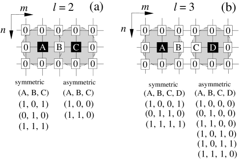
Figure 6: Modes supported by the moderately localized nonlinearity in the anticontinuum limit, for $l=2$ and $3$. Gray circles schematically indicate the localization of the nonlinearity.

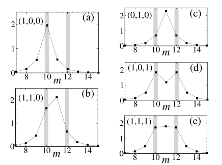
Figure 7: Modes supported by the moderately localized nonlinearity ($\Delta W=1$) at $l=2$ and $\omega=1$.

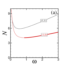
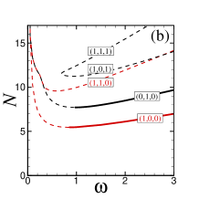
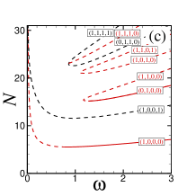
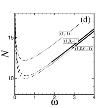
Figure 8: (Color online) Curves $N(\omega)$ for families of localized symmetric, asymmetric and antisymmetric modes, supported by the moderately localized nonlinearity, with $\Delta W=1$, for $l=1,\ 2$ and $3$. In (a)-(c) the black and red colors correspond to symmetric and asymmetric modes, respectively. Panel (d) shows the families of antisymmetric modes for different distances $l$.

This diagram is much richer than its counterpart in the case of the strong localization, cf. Fig. 2. In particular, two new branches of the solutions [symmetric ($0,1,0$) and asymmetric ($1,1,0$)] can be built in the ACL. In accordance with what said above, the partial delocalization of the nonlinearity makes it possible to construct ACL solutions that are localized not on the sites carrying the maximum nonlinearity, but on neighboring sites where the nonlinearity is also tangible, as shown in Fig. 1.

In the case of $l=1$ and weak localization, the situation is very similar to that corresponding to the strong localization. New types of bifurcations (actually, a bifurcation cascade) are found at larger $l$. For example, in the case of $l=2$, on the contrary to the situation corresponding to the strong localization, symmetric mode ($1,0,1$) does not have a small-amplitude limit, and disappears through a saddle-node bifurcation involving another symmetric mode ($1,1,1$) (which does not exist in the strong-localization model with $\Delta W=0.1$). The situation is different too in the small-amplitude limit (for small $\omega$). In Fig. 9(a), the existence curves for the symmetric and asymmetric solutions are presented in the region of small $\omega$. In panel (b) the profiles of symmetric ($0,1,0$) and asymmetric ($1,0,0$) and ($1,1,0$) modes are presented, before the first bifurcation. With the decrease of $\omega$, the first pitchfork bifurcation occurs between asymmetric mode ($1,1,0$) and symmetric one ($0,1,0$), transforming into a symmetric mode [see corresponding profiles at $\omega=0.2$ in Fig. 9(c)]. Later, symmetric mode ($0,1,0$) undergoes another pitchfork bifurcation with asymmetric mode ($1,0,0$). The final profile of the symmetric mode is shown in Fig. 9(d).

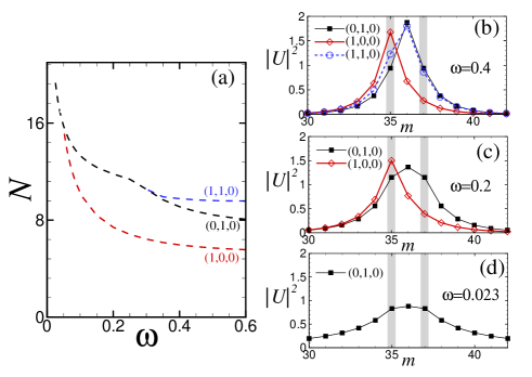
Figure 9: (Color online) In (a) the existence curves $N(\omega)$ from Fig. 8(b) are shown in the interval of $\omega\in[0,0.6]$. In (b)-(d), the profiles of the solutions at different propagation constants $\omega=0.4;0.2$ and $0.023$ are displayed. The gray stripes shows positions of the nonlinear spots.

By further increasing the distance between the nonlinear sites, $l$, the set of solution branches becomes even more complex. For instance, the system with $l=3$ shows a number of saddle-node bifurcations between modes ($1,1,0,1$) and ($1,0,1,0$), ($1,1,0,0$) and ($0,1,0,0$). Also, a more complex cascade of bifurcations occurs between modes ($1,1,1,1$) and ($1,1,1,0$) (pitchfork) and, further, with mode ($0,1,1,0$) (saddle-node). The linear stability analysis, displayed in Fig. 8, shows some noteworthy effects, such as an additional stable asymmetric branch ($0,1,0,0$).

5 Vortices supported by the localization of the nonlinearity

Dealing with the 2D model, it is natural too to explore symmetric and asymmetric vortices supported by the localized nonlinearity. In contrast to the localized modes without vorticity, the localization strength plays a crucial role for them [27, 1].

We are looking for vortical solution to the Eq. (3) starting from the ACL, as it was done in the previous section. The initial distribution of the exited sites in the ACL, designated as $\pm A,\pm B$, and the final shape of the symmetric (with $A=B=1$) and asymmetric ($A=1$ and $B\ll 1$) vortices, represented by $|U_{m,n}|^{2}$ with $\Delta W=1$ and distance $l=2$, are shown in Fig. 10. In Figs. 11 and 12, the existence of the symmetric and asymmetric vortices for different distances between nonlinear sites $l$ with fixed $\Delta W=1$ [panel (a)], and different width $\Delta W$ with fixed $l=2$ [panel (b)], are presented.

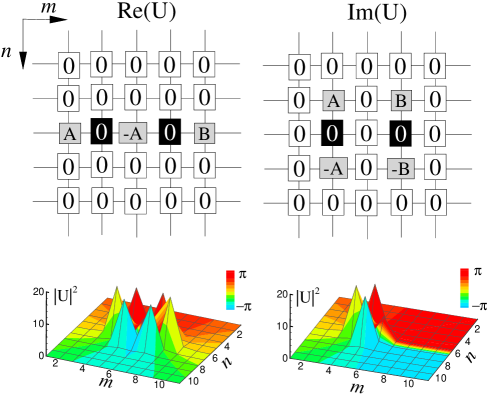
Figure 10: (Color online) Top row shows a schematic distribution of the exited sites in the real and imaginary parts of the vortex solution in the ACL. In the bottom row, the profiles of $|U_{m,n}|^{2}$ are shown for the symmetric (left, and asymmetric (right) vortices. The color gradient shows the phase distribution. Parameters are $\omega=2$, $l=2$, $\Delta W=1$.

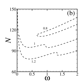
Figure 11: Curves representing families of symmetric vortices with different combination of the width of the nonlinear spots, $\Delta W$, and distance between them, $l$. In (a) $\Delta W=1$ and $l=2,3,4$, while in panel (b) $l=2$ and $\Delta W=0.8;1;1.2$.

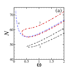
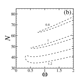
Figure 12: (Color online) The same as in Fig. 11, but for asymmetric vortex solutions. The colors and symbols in (a) allow to follow the overlapping existence curves.

According to the linear stability analysis (also verified by the direct simulations), symmetric and asymmetric vortices with different $l$ and $\Delta W$ are unstable. This may be explained by the fact that the spread of the nonlinearity is not sufficient for the creation of stable discrete vortices, whose stability region is narrow in the model with the uniform onsite nonlinearity [27].

6 Conclusion

In this work we have introduced the 2D lattice model, based on the linear discrete Schrödinger equation with two nonlinear sites embedded into it, and a generalization for the moderately localized nonlinearity with two separated maxima. The setting may be implemented in arrays of optical waveguides, and in BEC trapped in a deep optical-lattice potential. The existence and stability of discrete 2D solitons of the symmetric, antisymmetric, and asymmetric types have been considered in these systems. The setting with the moderate localization of the nonlinearity admits a much greater variety of the localized modes. The subcritical bifurcation, which accounts for the transition from symmetric to asymmetric modes, has been identified. In the case of the moderate localization, the existence and stability of discrete symmetric and asymmetric vortices have been also discussed.

References

- [1] P. G. Kevrekidis, The Discrete Nonlinear Schrödinger Equation: Mathematical Analysis, Numerical Computations, and Physical Perspectives (Springer: Berlin and Heidelberg, 2009).
- [2] M. I. Molina, G. P. Tsironis, Phys. Rev. B 47 (1993) 15330 (1993); B. C. Gupta, K. Kundu, Phys. Rev. B 55 (1997) 894.
- [3] V. A. Brazhnyi, B. A. Malomed, Phys. Rev. A 83 (2011) 053844.
- [4] B. Maes, M. Soljačić, J. D. Joannopoulos, P. Bienstman, R. Baets, S.-P. Gorza, M. Haelterman, Opt. Express, 14 (2006) 10678; E. N. Bulgakov, A. F. Sadreev, Phys. Rev. B 81 (2010) 115128; E. Bulgakov, A. Sadreev, K. N. Pichugin, ibid. B 83 (2011) 045109.
- [5] F. Lederer, G. I. Stegeman, D. N. Christodoulides, G. Assanto, M. Segev, Y. Silberberg, Phys. Rep. 463 (2008) 1.
- [6] A. A. Sukhorukov, A. S. Solntsev, S. S. Kruk, D. N. Neshev, and Y. S. Kivshar, Opt. Lett. 39 (2014) 462.
- [7] A. Trombettoni, A. Smerzi, Phys. Rev. Lett. 86, 2353 (2001); A. Smerzi, A. Trombettoni, Phys. Rev. A 68, 023613 (2003); F. Kh. Abdullaev, B. B. Baizakov, S. A. Darmanyan, V. V. Konotop, M. Salerno, Phys. Rev. A 64, 043606 (2001); A. Smerzi, A. Trombettoni, P. G. Kevrekidis, A. R. Bishop, Phys. Rev. Lett. 89, 170402 (2002); V. Ahufinger1 A. Sanpera, P. Pedri, L. Santos, M. Lewenstein, Phys. Rev. A 69 (2004) 053604; V. A. Brazhnyi, V. V. Konotop, V. M. Pérez-García, ibid. 74 (2006) 023614.
- [8] D. Jaksch, P. Zoller, Ann. Phys. 315 (2005) 52; M. Lewenstein, A. Sanpera, V. Ahufinger, B. Damski, A. Sen, U. Sen, Advances in Physics 56 (2007) 243; B. Ilan, M. I. Weinstein, Multiscale Model. Simul. 8 (2010) 1055.
- [9] P. Windpassinger, K. Sengstock, Rep. Prog. Phys. 76 (2013) 086401.
- [10] B. A. Malomed, E. Ding, K. W. Chow, S. K. Lai, Phys. Rev. E 86, 036608 (2012); K. W. Chow, E. Ding, B. A. Malomed, A. Y. S. Tang, Eur. Phys. J. Special Topics 223 (2014) 63.
- [11] S. Giorgini, L. P. Pitaevskii, and S. Stringari, Rev. Mod. Phys. 80 (2008) 1215; H. T. C. Stoof, K. B. Gubbels, D. B. M. Dickrsheid, Ultracold Quantum Fields (Springer: Dordrecht, 2009).
- [12] E. Díaz, C. Gaul, R. P. A. Lima, F. Domínguez-Adame, and C. A. Müller, Phys. Rev. A 81 (2010) 051607(R); G. A. Sekh, Phys. Lett. A 376 (2012) 1740.
- [13] R. Yamazaki, S. Taie, S. Sugawa, Y. Takahashi, Phys. Rev. Lett. 105 (2010) 050405.
- [14] G. Herring, P. G. Kevrekidis, B. A. Malomed, R. Carretero-González, D. J. Frantzeskakis, Phys. Rev. E 76 (2007) 066606.
- [15] Lj. Hadžievski, G. Gligorić, A. Maluckov, and B. A. Malomed, Phys. Rev. A 82 (2010) 033806.
- [16] G. Iooss and D. D. Joseph, Elementary Stability Bifurcation Theory (Springer-Verlag: New York, 1980).
- [17] V. A. Brazhnyi, B. A. Malomed, Phys. Rev. A 86 (2012) 013829.
- [18] T. Mayteevarunyoo, B. A. Malomed, G. Dong, Phys. Rev. A 78 (2008) 053601 (2008); N. Dror, B. A. Malomed, ibid. A 83 (2011) 033828 (2011); X.-F. Zhou, S.-L. Zhang, Z.-W. Zhou, B. A. Malomed, H. Pu, ibid. A 85 (2012) 023603.
- [19] A. Shapira, N. Voloch-Bloch, B. A. Malomed, A. Arie, J. Opt. Soc. Am. B 28 (2011) 1481.
- [20] T. Mayteevarunyoo, B. A. Malomed, A. Reoksabutr, J. Mod. Opt. 58 (2011) 1977.
- [21] Y. V. Kartashov, B. A. Malomed, Torner, Rev. Mod. Phys. 83 (2011) 247.
- [22] A. Szameit, J. Burghoff, T. Pertsch, S. Nolte, A. Tünnermann, Lederer, Opt. Exp. 14 (2006) 6055; A. Szameit, S. Nolte, J. Phys. B: At. Mol. Opt. Phys. 43 (2010) 163001.
- [23] J. Hukriede, D. Runde, D. Kip, J. Phys. D: Appl. Phys. 36 (2003) R1.
- [24] Z. Shi, J. Wang, Z. Chen, and J. Yang, Phys. Rev. A 78 (2008) 063812.
- [25] T. Dohnala, H. Uecker, Physica D 238 (2009) 860.
- [26] M. Vakhitov, A. Kolokolov, Radiophys. Quantum. Electron. 16 (1973)783 (1973); L. Bergé, Phys. Rep. 303 (1998) 259.
- [27] B. A. Malomed and P. G. Kevrekidis, Phys. Rev. E 64 (2001) 026601.