Causality between time series

Abstract

Given two time series, can one tell, in a rigorous and quantitative way, the cause and effect between them? Based on a recently rigorized physical notion namely information flow, we arrive at a concise formula and give this challenging question, which is of wide concern in different disciplines, a positive answer. Here causality is measured by the time rate of change of information flowing from one series, say, $X_{2}$, to another, $X_{1}$. The measure is asymmetric between the two parties and, particularly, if the process underlying $X_{1}$ does not depend on $X_{2}$, then the resulting causality from $X_{2}$ to $X_{1}$ vanishes. The formula is tight in form, involving only the commonly used statistics, sample covariances. It has been validated with touchstone series purportedly generated with one-way causality. It has also been applied to the investigation of real world problems; an example presented here is the cause-effect relation between two climate modes, El Niño and Indian Ocean Dipole, which have been linked to the hazards in far flung regions of the globe, with important results that would otherwise be difficult, if not impossible, to obtain.

I Introduction

Causality identification between dynamical events is a subject of great interest in different disciplines. Examples are seen everywhere in neurosciencePereda Korz03 Wu Baptista , biologySachs Okasha Jost , social and computer network dynamicsAy Sommerlade , financial economicsChenCR Lee , statistical physicsCrutchfield , to name a few. Toward the end of this study, we will see a climate science problem that has been linked to the severe weather and natural disasters on a global scale.

Given that, more often than not, what is known about the two events in question are in the form of time series, causality analysis between time series is therefore of particular importance. Presently a common practice in applied sciences, e.g., climate science, is through computing time-lagged correlation. However, it is well known that correlation does not carry the needed directedness or asymmetry and hence does not necessarily imply causality. Besides, it is easy to argue that, for recurrent processes, there is actually no way to distinguish a lag from an advance, unless one has enough a priori knowledge of the processes of concern. This is particularly a problem when the processes are nonsequential (e.g., those in the nonsequential stochastic control systems). Another common practice is through Granger causality test, which is a statistical test of the usefulness of one time series in forecasting another. This kind of test, as the name implies, provides only a yes/no judgment, lacking the quantitative information that may be required in many circumstances.

On the other hand, information flow, or information transfer as it may be referred to in the literature, provides such a quantitative measure; the amount of information exchange between two events offers not only the direction but also the magnitude of the cause-effect relation. Due to its importance, the past decades have seen a surge of interest in formulating this notion. Formalisms have been established empirically or half-empirically, and have been used for different researches, among which is transfer entropySchreiber . Realizing that information flow is a real physical notion, and that a real physical notion should be rigorously, rather than empirically, built on a solid foundation so as to be universally applicable for problems in different disciplines, Liang and KleemanLK05 take the initiative to establish, followed by a series of researches afterwards, a rigorous formalism for the information flow within given dynamical systems, both deterministic and stochastic systems (see Liang13 for a review). The problem now is whether and how the same notion can be translated to cases with no dynamics but time series previously given; that way, the quantitative causal relation between the series will be obtained. In some sense this is an inverse problem, and could be challenging since no a priori knowledge of the dynamics is available. In the following we first briefly introduce the Liang-Kleeman information flow within a two-dimensional system (section II). The major derivation is presented in section III, where a concise formula for causality analysis is obtained. This formula is validated with touchstone time series purportedly generated with only one-way causality (section IV); it is then applied to the study of the causal relation between El Niño and Indian Ocean Dipole (IOD), the two major modes of climate variation, with important results which have been evidenced for years but missed in previous analyses with existing tools (section V).

II Liang-Kleeman information flow

Let us begin with a brief introduction of the Liang-Kleeman information flow. Consider a $d$-dimensional stochastic system

$$d{\bf X}={\bf F}({\bf X};{\bm{\theta}})dt+{\bf{B}}({\bf X};{\bm{\theta}})d{\bf W}$$ (1)

where ${\bf F}$ is the vector of drift coefficients, ${\bf{B}}=(b_{ij})$ a matrix of diffusion coefficients (or volatility in finance), and ${\bf W}$ a vector of standard Wiener process ($\dot{{\bf W}}$ is the so-called white noise). The rate of information flowing from a component, say, $X_{2}$ to another, say, $X_{1}$, is the change rate of the marginal entropy of $X_{1}$, minus the same change rate but with the effect from $X_{2}$ instantaneously excluded from the system. These rates of information flow/transfer have been obtained analytically in a closed form for any given dynamical systemsLiang08 ; particularly, for a system of dimensionality 2, which we will be considering in this study, the flow rate from $X_{2}$ to $X_{1}$ is

$${T}_{2\to 1}=-E\left(\frac{1}{\rho_{1}}\frac{\partial(F_{1}\rho_{1})}{\partial x_{1}}\right)+\frac{1}{2}E\left(\frac{1}{\rho_{1}}\frac{\partial^{2}(b_{11}^{2}+b_{12}^{2})\rho_{1}}{\partial x_{1}^{2}}\right),$$ (2)

where $\rho_{1}$ is the marginal probability density of $X_{1}$, and $E$ the mathematical expectation. ${T}_{2\to 1}$ may be either zero or nonzero. A nonzero ${T}_{2\to 1}$ means that $X_{2}$ is causal to $X_{1}$: a positive value means that $X_{2}$ makes $X_{1}$ more uncertain, and vice versa. This measure of information flow possesses an important property, namely the property of flow/transfer asymmetry: One-way information flow implies nothing about the transfer in the opposition direction. A very particular case is: when the evolution of $X_{1}$ does not depend on $X_{2}$, ${T}_{2\to 1}=0$ (see Liang13 for proofs in different situations). Considering its criticality, this property makes a touchstone for the testing of causality analysis tools.

III Causality analysis

Shown above are some of the theoretical results of the Liang-Kleeman information flow for 2D systems. These results are rigorous, but the formalism is not about causality analysis, as the causal relation is prescribed in the given system. We need to develop an analysis without a priori knowledge of the dynamics; the only given conditions are the two time series. To some extent this is like an inverse problem. Generally it could be very challenging, considering the touchstone property, among others, to be verified.

Since the dynamics is unknown, we need to choose a model first. As always, a linear model is the natural choice. In Eq. (1), assume ${\bf F}={\bf f}+{\bf{A}}{\bf X}$, with ${\bf f}=({f_{1}},{f_{2}})^{T}$, ${\bf{A}}=(a_{ij})$, and ${\bf{B}}=(b_{ij})$ being constant vector/matrices. In the equation, suppose that initially $(X_{1},X_{2})$ has a bivariate normal distribution. As the system is linear, then the density is always normalLasota . Denote the mean by ${\bm{\mu}}=(\mu_{1},\mu_{2})^{T}$, and the covariance matrix by ${\bm{\Sigma}}=(\sigma_{ij})$. They evolve following the differential equations

$$\frac{d{\bm{\mu}}}{dt}={\bf f}+{\bf{A}}{\bm{\mu}},$$ (3)

$$\frac{d{\bm{\Sigma}}}{dt}={\bf{A}}{\bm{\Sigma}}+{\bm{\Sigma}}{\bf{A}}^{T}+{\bf{B}}{\bf{B}}^{T}.$$ (4)

The information flows between $X_{1}$ and $X_{2}$ are now easy to evaluate. Consider ${T}_{2\to 1}$ first. When $(b_{ij})$ are constant, the last term of (2) vanishes, thanks to a nice property proved in Liang08 . Substitution of

$$F_{1}=f_{1}+a_{11}X_{1}+a_{12}X_{2}$$ (5)

$$\rho_{1}=\frac{1}{\sqrt{2\pi}\sigma_{1}}e^{-\frac{(x_{1}-\mu_{1})^{2}}{2\sigma_{1}^{2}}}$$ (6)

into (2) for $F_{1}$ and $\rho_{1}$ yields, after some algebraic manipulations,

$${T}_{2\to 1} = \frac{\sigma_{12}}{\sigma_{11}}a_{12},$$ (7)

where $\sigma_{ij}$ is obtained by solving (4). (Note that extra terms will be involved if ${\bf{B}}$ depends on ${\bf X}$.) Likewise,

$${T}_{1\to 2} = \frac{\sigma_{12}}{\sigma_{22}}a_{21}.$$ (8)

For an example, consider the case ${\bf f}={\bf 0}$, ${\bf{A}}=\left[\begin{array}[]{ll}-1&0.5\\ 0&-1\end{array}\right]$, ${\bf{B}}=\left[\begin{array}[]{ll}0.1&0\\ 0&0.1\end{array}\right]$, which gives a 2D stochastic differential equation (SDE):

$$dX_{1}=(-X_{1}+0.5X_{2})dt+0.1dW_{1},$$ (9)

$$dX_{2}=-X_{2}dt+0.1dW_{2}.$$ (10)

Clearly, $X_{2}$ drives $X_{1}$, but not vice versa. The computed rates of information flow are shown in Fig. 1. As expected, $T_{1\to 2}\equiv 0$, since the evolution of $X_{2}$ does not depend on $X_{1}$. That is to say, to $X_{2}$, $X_{1}$ is not causal. On the other hand, $X_{2}$ drives $X_{1}$ and hence is causal to $X_{1}$; correspondingly $T_{2\to 1}\neq 0$. In this example, $T_{2\to 1}$ approaches a constant 0.1111 no matter how the system is initialized, though the result may be different during the spin-up period. This kind of example is very typical in causality analysis: One component causes another, but the latter has no feedback to the former. Later we will use it to test our causality analysis.

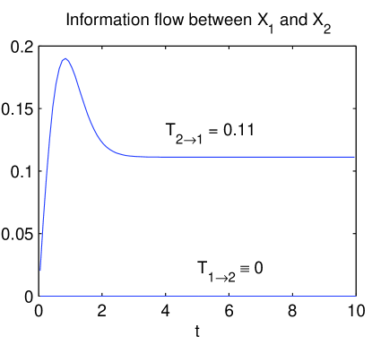
Figure 1: Accurate result of the information flow between $X_{1}$ and $X_{2}$ within the linear system (9)-(10). The variance is initialized with $\sigma_{11}=\sigma_{22}=0.1$, $\sigma_{12}=0$.

Our strategy to approach the problem is first to estimate the linear model, i.e., to estimate the parameters $({\bf f},{\bf{A}},{\bf{B}})$, which we will be symbolically writing as ${\bm{\theta}}$, with the time series, and then compute the information flow. To further simplify the problem, let ${\bf{B}}=\left[\begin{array}[]{ll}b_{1}&0\\ 0&b_{2}\end{array}\right],$ and assume that the time series are equal-distanced.

We use maximum likelihood estimation (mle) to fulfill the purpose. Consider an interval $[n{\Delta t},(n+1){\Delta t}]$, ${\Delta t}$ being the time stepsize. If the transition probability density function $\rho({\bf X}_{n+1}|{\bf X}_{n};{\bm{\theta}})$ can be obtained, since $\{X_{n}\}$ is a Markov process, the likelihood

$$L_{N}({\bm{\theta}})=\rho({\bf X}_{1})\cdot\rho({\bf X}_{2}|{\bf X}_{1};{\bm{\theta}})...\rho({\bf X}_{N}|{\bf X}_{N-1};{\bm{\theta}})$$ (11)

is then given ($N$ the sample size), or, alternatively, the log likelihood

$$\ell_{N}({\bm{\theta}})=\sum_{n=1}^{N}\log\rho({\bf X}_{n+1}|{\bf X}_{n};{\bm{\theta}})+\log\rho({\bf X}_{1})$$ (12)

is obtained. When $N$ is large, $\rho({\bf X}_{1})$ can be dropped without causing much error. In this linear case, analytical solution of $\rho$ can be found; the result, however, is complicated. In the interest of applicability, we turn to the discretized version of the SDE. Using the Euler-Bernstein scheme (cf. Lasota ),

$${\bf X}_{n+1}={\bf X}_{n}+{\bf F}({\bf X}_{n};{\bm{\theta}}){\Delta t}+{\bf{B}}({\bf X}_{n};{\bm{\theta}})\Delta{\bf W},$$ (13)

where $F={\bf f}+{\bf{A}}{\bf x}$. Suppose ${\Delta t}$ is small, we know

$$\Delta{\bf W}\ \sim\ {\mathscr{N}}({\bf 0},\ {\bf{B}}{\bf{B}}^{T}{\Delta t}),$$

$${\bf X}_{n+1}|{\bf X}_{n}={\bf x}_{n}\ \sim\ {\mathscr{N}}({\bf x}_{n}+{\bf F}{\Delta t},\ {\bf{B}}{\bf{B}}^{T}{\Delta t}).$$

So

$$\rho({\bf X}_{n+1}={\bf x}_{n+1}|{\bf X}_{n}={\bf x}_{n})$$

$$=\frac{1}{\left[(2\pi)^{2}\det({\bf{B}}{\bf{B}}^{T}{\Delta t})\right]^{1/2}}e^{-\frac{1}{2}({\bf x}_{n+1}-{\bf x}_{n}-{\bf F}{\Delta t})^{T}({\bf{B}}{\bf{B}}^{T}{\Delta t})^{-1}({\bf x}_{n+1}-{\bf x}_{n}-{\bf F}{\Delta t})},$$

and

$$\ell_{N}({\bm{\theta}})=\sum_{n=1}^{N}\log\rho({\bf X}_{n+1}|{\bf X}_{n};{\bm{\theta}})$$ (14)

$$={\rm const}-\frac{1}{2}\sum_{n=1}^{N}\log\left[\det({\bf{B}}{\bf{B}}^{T})\right]$$ (15)

$$\ \ \ -\frac{1}{2{\Delta t}}\sum_{n=1}^{N}({\bf x}_{n+1}-{\bf x}_{n}-{\bf F}{\Delta t})^{T}({\bf{B}}{\bf{B}}^{T})^{-1}({\bf x}_{n+1}-{\bf x}_{n}-{\bf F}{\Delta t}).$$ (16)

Note here we have assumed that $N$ is large enough such that $\rho(X_{1})$ can be dropped without causing much error. The mle of ${\bm{\theta}}$ is, therefore,

$${\bm{\hat{\theta}}}=\arg\max_{\theta}\ell_{N}({\bm{\theta}}).$$ (17)

For convenience, denote, for $i=1,2$,

$$\dot{X}_{i,n} := \frac{X_{i,n+1}-X_{i,n}}{{\Delta t}},$$ (18)

$$R_{i,n} := \dot{X}_{i,n}-(f_{i}+a_{i1}X_{1,n}+a_{i2}X_{2,n}).$$ (19)

Also notice that ${\bf{B}}{\bf{B}}^{T}=\left[\begin{array}[]{ll}b_{1}^{2}&0\\ 0&b_{2}^{2}\end{array}\right]$. Substituting into Eq. (16), the log likelihood $\ell_{N}({\bm{\theta}})=\ell_{N}({\bf f},{\bf{A}},{\bf{B}})$ is,

$$\ell_{N}({\bf f},{\bf{A}},{\bf{B}})={\rm const}-\frac{N}{2}\log b_{1}^{2}b_{2}^{2}-\frac{{\Delta t}}{2}\left[\frac{1}{b_{1}^{2}}\sum_{n=1}^{N}R_{1,n}^{2}+\frac{1}{b_{2}^{2}}\sum_{n=1}^{N}R_{2,n}^{2}\right]$$ (20)

The estimators of ${\bf f}$, ${\bf{A}}$, and ${\bf{B}}$ can be found by maximizing $\ell_{N}$. It is interesting to note that the equations governing the estimators $(\hat{f}_{1},\hat{a}_{11},\hat{a}_{12})$, $(\hat{f}_{2},\hat{a}_{21},\hat{a}_{22})$, and $(\hat{b}_{1},\hat{b}_{2})$ are actually decoupled. This makes the estimation much easier. Besides, notice that maximizing $\ell_{N}$ over $(f_{i},a_{i1},a_{i2})$ is equivalent to minimizing $\sum_{n}R_{i,n}^{2}:=Q_{N,i}$ over the same group of parameters, for $i=1,2$. So $(\hat{f}_{1},\hat{a}_{11},\hat{a}_{12})$ are precisely the least square estimators, which satisfies

$$\left[\begin{array}[]{lll}N&\sum X_{1,n}&\sum X_{2,n}\\ \sum X_{1,n}&\sum X_{1,n}^{2}&\sum X_{1,n}X_{2,n}\\ \sum X_{2,n}&\sum X_{2,n}X_{1,n}&\sum X_{2,n}^{2}\end{array}\right]\left[\begin{array}[]{l}\hat{f}_{1}\\ \hat{a}_{11}\\ \hat{a}_{12}\end{array}\right]=\left[\begin{array}[]{l}\sum\dot{X}_{1,n}\\ \sum X_{1,n}\dot{X}_{1,n}\\ \sum X_{2,n}\dot{X}_{1,n}\end{array}\right].$$

The above equation set can be written in a more familiar and succinct form:

$$\left[\begin{array}[]{lll}1&{\overline{X_{1}}}&{\overline{X_{2}}}\\ {\overline{X_{1}}}&{\overline{X_{1}^{2}}}&{\overline{X_{1}X_{2}}}\\ {\overline{X_{2}}}&{\overline{X_{1}X_{2}}}&{\overline{X_{2}^{2}}}\end{array}\right]\left[\begin{array}[]{l}\hat{f}_{1}\\ \hat{a}_{11}\\ \hat{a}_{12}\end{array}\right]=\left[\begin{array}[]{l}{\overline{\dot{X}_{1}}}\\ {\overline{X_{1}\dot{X}_{1}}}\\ {\overline{X_{2}\dot{X}_{1}}}\end{array}\right],$$ (31)

where, as usual, the overline signifies sample mean. After some algebraic manipulations, it becomes:

$$\left[\begin{array}[]{lll}1&{\overline{X_{1}}}&{\overline{X_{2}}}\\ 0&{\overline{X_{1}^{2}}}-\bar{X}_{1}^{2}&{\overline{X_{1}X_{2}}}-\bar{X}_{1}\bar{X}_{2}\\ 0&{\overline{X_{1}X_{2}}}-\bar{X}_{1}\bar{X}_{2}&{\overline{X_{2}^{2}}}-\bar{X}_{2}^{2}\end{array}\right]\left[\begin{array}[]{l}\hat{f}_{1}\\ \hat{a}_{11}\\ \hat{a}_{12}\end{array}\right]=\left[\begin{array}[]{l}{\overline{\dot{X}_{1}}}\\ {\overline{X_{1}\dot{X}_{1}}}-\bar{X}_{1}\bar{\dot{X}}_{1}\\ {\overline{X_{2}\dot{X}_{1}}}-\bar{X}_{2}\bar{\dot{X}}_{1}\end{array}\right].$$

Let

$$C_{ij}:={\overline{(X_{i}-\bar{X}_{i})(X_{j}-\bar{X}_{j})}},$$ (33)

$$C_{i,dj}:={\overline{(X_{i}-\bar{X}_{i})(\dot{X}_{j}-\bar{\dot{X}}_{j})}},$$ (34)

${\bf{C}}=(C_{ij})$ being the sample covariance matrix. The equation set is actually

$$\left[\begin{array}[]{lll}1&{\overline{X_{1}}}&{\overline{X_{2}}}\\ 0&C_{11}&C_{12}\\ 0&C_{12}&C_{22}\end{array}\right]\left[\begin{array}[]{l}\hat{f}_{1}\\ \hat{a}_{11}\\ \hat{a}_{12}\end{array}\right]=\left[\begin{array}[]{l}{\overline{\dot{X}_{1}}}\\ C_{1,d1}\\ C_{2,d1}\end{array}\right],$$

which yields

$$\hat{a}_{11}=\frac{C_{22}C_{1,d1}-C_{12}C_{2,d1}}{\det{\bf{C}}},$$ (36)

$$\hat{a}_{12}=\frac{-C_{12}C_{1,d1}+C_{11}C_{2,d1}}{\det{\bf{C}}},$$ (37)

$$\hat{f}_{1}=\bar{\dot{X}}_{1}-\hat{a}_{11}\bar{X}_{1}-\hat{a}_{12}\bar{X}_{2}.$$ (38)

The other group of estimators can be obtained by switching the indices:

$$\hat{a}_{22}=\frac{C_{11}C_{2,d2}-C_{12}C_{1,d2}}{\det{\bf{C}}},$$ (39)

$$\hat{a}_{21}=\frac{-C_{12}C_{2,d2}+C_{22}C_{1,d2}}{\det{\bf{C}}},$$ (40)

$$\hat{f}_{2}=\bar{\dot{X}}_{2}-\hat{a}_{21}\bar{X}_{1}-\hat{a}_{22}\bar{X}_{2}.$$ (41)

With these results, let $\frac{\partial\ell_{N}}{\partial b_{i}}=0$ to get

$$\hat{b}_{i}=\sqrt{\frac{Q_{N,i}\cdot{\Delta t}}{N}},$$ (42)

where

$$Q_{N,i}=\sum_{n=1}^{N}R_{i,n}^{2}=\sum_{n=1}^{N}\left[\dot{X}_{i,n}-(\hat{f}_{i}+\hat{a}_{i1}X_{1,n}+\hat{a}_{i2}X_{2,n})\right]^{2}.$$

On the other hand, as the population covariance matrix can be estimated by the sample covariance matrix, the estimator of $\sigma_{12}/\sigma_{11}$ is $C_{12}/C_{11}$. Substituting these results back to (7), we finally obtain the rate of information flowing from $X_{2}$ to $X_{1}$:

$$\boxed{{T}_{2\to 1}=\frac{C_{12}}{C_{11}}\cdot\frac{-C_{12}C_{1,d1}+C_{11}C_{2,d1}}{C_{11}C_{22}-C_{12}^{2}},}$$ (43)

where $C_{ij}$ is the sample covariance between $X_{i}$ and $X_{j}$, and $C_{i,dj}$ the covariance between $X_{i}$ and $\dot{X}_{j}$. Strictly speaking, here $T_{2\to 1}$ should bear a caret since it is an estimator of the true information flow. But we will abuse the notation a little bit for the sake of terseness. The flow in the opposite direction, $T_{1\to 2}$, can be directly written out by switching the indices 1 and 2. The units are in nats per unit time.

Given a significance level, we may estimate the confidence interval for (43). This can always be achieved with bootstrap. But here things can be simplified. When $N$ is large, $T_{2\to 1}$ is approximately normally distributed around its true value with a variance $\left(\frac{C_{12}}{C_{11}}\right)^{2}\hat{\sigma}^{2}_{a_{12}}$, thanks to the mle property. Here $\hat{\sigma}^{2}_{a_{12}}$ is determined as follows. Denote ${\bm{\theta}}=(f_{1},a_{11},a_{12},b_{1})$. Compute

$$NI_{ij}=-\sum_{n=1}^{N}\frac{\partial^{2}\log\rho({\bf X}_{n+1}|{\bf X}_{n};\ \hat{{\bm{\theta}}})}{\partial\theta_{i}\partial\theta_{j}}$$ (44)

to form a matrix $N{\bf{I}}$, ${\bf{I}}$ being the Fisher information matrix. The inverse $(N{\bf{I}})^{-1}$ is the covariance matrix of $\hat{{\bm{\theta}}}$, within which is $\hat{\sigma}_{a_{12}}^{2}$. Given a significance level, the confidence interval can be found accordingly.

IV Validation

The above formula is remarkably tight in form, involving only the common statistics namely sample covariance matrix. We now check whether they verify the example shown in Fig. 1. The data we have is just one realization, i.e., one sample path of $X_{1}$ and $X_{2}$ each generated from the given system. Using a time step ${\Delta t}=0.001$, we generate 100000 steps, corresponding to a time span $t=0-100$. For later use, we purportedly initialize the series far from the equilibrium to allow for a period of spin-down, as shown in Fig. 2. The series reach a stationary state after approximately $t=4$; shown in the inserted box is a close-up plot. Our objective is, of course, not to estimate the whole evolution course as shown in Fig. 1; what we expect is to see whether the stationary values ($T_{2\to 1}=0.1111$, $T_{1\to 2}=0$) can be estimated with acceptable confidence. For this purpose, we form different series from the sample path with different resolutions and different time intervals and lengths, and then test the performance of estimation. The testing results are listed in Table 1.

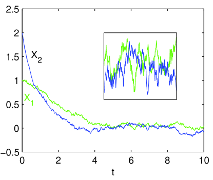
Figure 2: A sample path of the linear SDE (9)-(10) generated using the Euler-Bernstein scheme with ${\Delta t}=0.001$ and initialized with $(1,2)$. Inserted is a close-up over the interval $t=4.5$-$8.5$.

Table 1: The information flow computed with different series formed by sampling from the path shown in Fig. 2. $\Delta n$ is the sampling interval. The accurate result is: $T_{2\to 1}=0.1111$, $T_{1\to 2}=0$ (in nats per unit time). In the last two cases, data on $[5,10]$ are used to compute $C_{ij}^{*}$.

Time span	$\Delta n$	$T_{2\to 1}$	$T_{1\to 2}$	Remark
$t$=5-100	1	0.11	$-2.0\times 10^{-3}$
	20	0.10	$-4.0\times 10^{-3}$
	100	0.09	-0.01
$t$=10-20	1	0.60	0.17
	10	0.57	0.20
$t$=0-10	1	0.74	0.10
	1	0.29	0.02	use (45)
	10	0.28	0.02	use (45)

Clearly, so long as the time span of the series is long enough, the estimation can be made rather accurate. With stationary data ($t=5-100$), even when one samples the path every 100 time steps (corresponding to a time resolution of 0.1) which yields a time series of only 1000 data points, the result is still acceptable to some extent. In some cases, the span may not be that long. To see how the formula may perform, we make two series spanning only 10 time units. In the first case we test with a stationary segment $t=10-20$. The result: $T_{2\to 1}=0.60$, $T_{1\to 2}=0.17$, unfortunately, is not as good as one would like to expect, even though the data points amount to 10000. Nonetheless, if we estimate the standard error at a 95% significance level, which gives a value of 0.54 and 0.47, respectively, the result still sounds informative. It tells that $T_{2\to 1}$ is significantly (at a 95% level) greater than zero, while $T_{1\to 2}$ is not significantly different from zero, consistent with the accurate result.

On the other hand, if the time span, though small, contains the nonstationary period, things may actually turn better. Choose an interval $t=0-10$. The result looks remarkably promising, provided that we treat the covariances in the first fraction of (43) and that in the second fraction differently. In the first fraction, the sample covariances are indeed used to estimate the populate covariances, and hence cannot be computed with the nonstationary data. In the second fraction, the mle is for the deterministic coefficient and so nonstationary data could serve the purpose better (indeed this is true). To distinguish these two different estimations, we denote the former with an asterisk; in doing so the formula (43) now looks

$${T}_{2\to 1}=\frac{C_{12}^{*}}{C_{11}^{*}}\cdot\frac{-C_{12}C_{1,d1}+C_{11}C_{2,d1}}{C_{11}C_{22}-C_{12}^{2}}.$$ (45)

Now go back to the chosen time series spanning $[0,10]$. If $C_{ij}^{*}$ are computed with data on $[5,10]$, then the one-way causality between the two series actually can be fairly reproduced, though the resulting $T_{2\to 1}$ is 1.6 times larger. Moreover, this result is very robust even the resolution is reduced by ten times. If one only considers a qualitative causal relation, this example shows that our approach is promising even when the length of the time series is limited.

We have tested the formula against systems with different drift and diffusion coefficients, particularly systems where noises dominate. Again, so long as the series have a span long enough, the causal relation can be faithfully reproduced. As an example, for the system

$$dX_{1}=-0.5X_{1}+X_{2}+20dW_{1},$$

$$dX_{2}=-0.7X_{2}+10dW_{2},$$

if the series span 1000 time units or longer, the estimation of $T_{2\to 1}$ and $T_{1\to 2}$ can be made fairly accurate.

V An application example

Finally let us look at an application to a real world problem: the causal relation between the two famous climate modes, El Niño and Indian Ocean Dipole (IOD). El Niño is the strongest interannual climate variation in the tropical Pacific air-sea coupled system, occurring at irregular intervals of 2 to 7 years and lasting 9 months to 2 yearsCane83 ; it is well known through its linkage to natural disasters in far flung regions of the globe, such as the floods in Ecuador, the droughts in Southeast Asia and Southern Africa, the increased number of storms over the Pacific Ocean. There are several indices measuring the strength of El Niño , the popular ones being Niño3 and Niño4Trenberth97 . IOD is another air-sea coupled climate mode, characterized by an aperiodic oscillation of sea surface temperature (SST) in the Indian OceanSaji99 . It has been related to, among others, the floods in East Africa and drought in Indonesia and parts of Australia. IOD is measured by an index called Dipole Mode Index (DMI).

As the dominant modes in respectively Pacific and Indian Oceans, the relationship between El Niño and IOD is of substantial interest; see Wang04 for an excellent review. It has long been recognized that the tropical Indian and Pacific Oceans are interrelatedKiladis on their SST anomalies. But the relation between the two modes is still to be clarified. In general, it is believed that El Niño may induce IOD, which usually peaks in fall; a recent study is referred to Wang13 . The causality of El Niño is easily understandable, considering the alteration of the Walker circulation during the El Niño years which causes the subsidence over the Indian Ocean (e.g., Klein99 ). On the other hand, the impact from the IOD has jut been recognized recently; in fact, in early efforts, Indian Ocean used to be treated as a slab of mixed layer responding passively to El Niño Lau00 . The recognition is mainly through climate predictions, such as the El Niño predictions (e.g., Chen08 , Izumo14 ) and the CGCM experiments (e.g., Annamalai10 ). Due to the correlation between the two modes, it has been suggested that an Indo-Pacific perspective should be adopted in researching on the El Niño and IOD problems (e.g., Webster10 )

The linkage between IOD and El Niño , though evidenced from different aspects, is somewhat still an issue in debate. This is partly due to the failure to recover the IOD pattern in the Indian Ocean in many correlation or time-lagged correlation analyses with the indices and the SST observations, albeit the correlation could be significant. Such an example is shown in the Fig.4 of Wang et al. (2004). This has led people to conclude with caution that IOD might be partially independent of El Niño , though El Niño tends to induce IOD. This problem, which is obviously a problem on cause and effect, could be due to the inadequacy of using correlation analysis for causality purposes. Now that we have arrived at the formula (43), let us see how things will come out when it is applied to the IOD-El Niño causality analysis.

First look at the causal relation between the indices of the two modes. The DMI used is the monthly series by Japan Agency for Marine-Earth Science and Technology (JAMSTEC), which can be downloaded from their website. The El Niño indices are from NOAA ESRL Physical Sciences Division (http://www.esrl.noaa.gov/psd/); they are also monthly data. Since this DMI series spans from January 1958 to September 2010, the El Niño indices, which have a much longer time span (1870-present), are also tailored to the same period. These series then have a total of 633 time points. Application of (43) to the DMI and Niño4 yields a flow of information from El Niño to IOD: $T_{E\to I}=-6$, and a flow from IOD to El Niño : $T_{I\to E}=13$ (units: $10^{-3}$ nats/month). Using Niño3 one arrives at a similar result: $T_{E\to I}=-6$ and $T_{I\to E}=16$. That is to say, El Niño and IOD are mutually causal, and the causality is asymmetric, with the one from the latter to the former larger than its counterpart. Moreover, the different signs indicate that El Niño tends to stabilize IOD, while IOD tends to make El Niño more uncertain.

By our previous experience, series length is crucial. To see whether the length here is adequate, we have tried shortened series: 1963-2010, 1968-2010. The former yields essential the same result as the one in its full length (1958-2010); the result of the latter is also similar. In fact, even series with a span as short as 1970-2010 can give qualitatively similar result. So the series may be long enough to form an ensemble with sufficient statistics. The resulting information flow rates hence may be acceptable.

With this assertion we proceed to extract the causality patterns out of the SST in the Pacific and Indian Oceans. The SST data are from the above NOAA site. As before, we use only the data for the period 1958-2010. First, compute the causality between DMI and the tropical Pacific SST. The results are shown in Fig. 3. Clearly DMI and the Pacific SST are mutually causal, and the information flow in either direction has a El Niño -like pattern. The signs of the flows are the same as computed above with two index series.

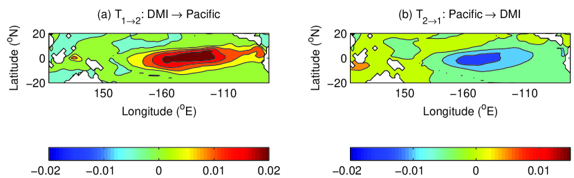
Figure 3: Information flow between DMI and the tropical Pacific SST (in nats/month).

If the above El Niño -like pattern in the Pacific is common, the following pattern in the Indian Ocean is unique to our causality analysis. Compute the information flow between Niño4 and the Indian Ocean SST, and plot the result in Fig. 4. Fig. 4a shows the flow from El Niño to the SST. In the tropical region, there are indeed two poles, though the eastern one covers a rather limited region over Indonesia. On the map of the feedback from the Indian Ocean SST (Fig. 4b), this structure is much clear, with a dipole pattern reminiscent of IOD, though there seems to be a shift eastward. This is remarkable, as in previous correlation analyses or time-lagged correlation analyses, the IOD pattern is not seen. Note in Fig. 4b, both centers are positive, indicating that the Indian Ocean influences the El Niño through IOD, which functions to amplify the El Niño oscillations. In contrast, the impact of El Niño on the Indian Ocean SST divides over the two centers, which have opposite signs of information flow. The causality analysis with Niño3 shows similar patterns, though the features may not be as pronounced as that with Niño4.

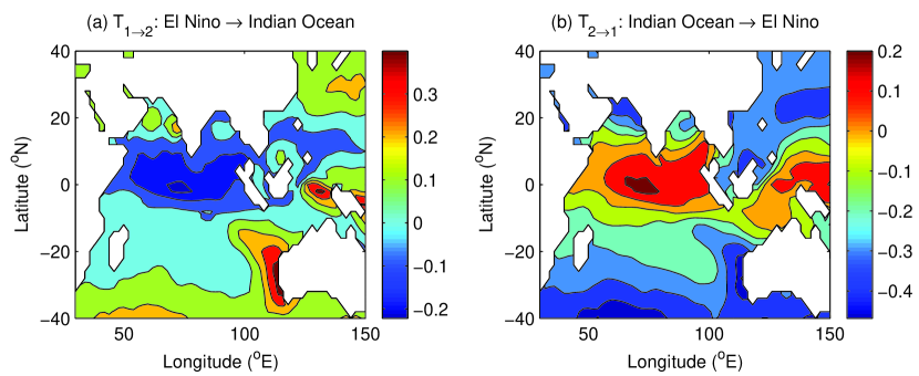
Figure 4: Information flow between Niño4 and the Indian SST (units: nats/month).

The relation between El Niño and IOD is an extensively investigated subject; further discussion, however, is beyond the scope of this study. Our purpose here is to use it as one real world example to demonstrate the utility of the newly derived formula (43). The result is encouraging: the IOD-like pattern, which is anticipated as evidence builds up, but missed in previous correlation studies, is recovered faithfully in the index-SST causality patterns. Moreover, it is found that, on the whole, the El Niño influences the IOD by making the latter more certain, while the causality from IOD to El Niño is generally the opposite. This is perhaps the reason why it has long been observed in a definite way that El Niño may induce IOD, while the influence from IOD to El Niño , albeit stronger, has been just recognized recently through predictability studies. The latter, which carries a positive information of flow, means that, to El Niño , the Indian Ocean is a source of uncertainty, and the causality from IOD to El Niño is manifested as a transference of uncertainty from the former to the latter. Clearly an efficient way to observe and forecast an event is to put extensive observation at its uncertainty source–a way how target observing systems are designed. This is why knowledge of the Indian Ocean facilitates the El Niño forecast (e.g., Chen08 , Izumo14 ), i.e., increases the predictability of El Niño .

VI Discussion

We have obtained, based on a rigorous formalism of information flow, a concise formula for causality analysis between time series. For series $X_{1}$ and $X_{2}$, the rate of information flowing (units: nats per unit time) from the latter to the former is

$${T}_{2\to 1}=\frac{C_{12}}{C_{11}}\cdot\frac{C_{11}C_{2,d1}-C_{12}C_{1,d1}}{C_{11}C_{22}-C_{12}^{2}},$$ (46)

where $C_{ij}$ is the sample covariance between $X_{i}$ and $X_{j}$, $C_{i,dj}$ the covariance between $X_{i}$ and $\dot{X}_{j}$, and $\dot{X}_{j}$ the difference approximation of $\frac{dX_{j}}{dt}$ using the Euler forward scheme [see Eq. (18)]. If $T_{2\to 1}=0$, $X_{2}$ does not cause $X_{1}$; if not, it is causal. In the presence of causality, two cases can be distinguished according to the sign of the flow: a positive $T_{2\to 1}$ means that $X_{2}$ functions to make $X_{1}$ more uncertain, while a negative value indicates that $X_{2}$ tends to stabilize $X_{1}$. The formula is very tight, involving only the common statistics namely the sample covariances. It has been validated with touchstone series, where the stationary preset one-way causality can be rather accurately recovered, provided that the series is long enough (time span, not number of data points) to contain sufficient statistics. When the series length is guaranteed, the formula works even with series with rather coarse resolution. Moreover, the series need not be stationary for the formula to apply; in fact, when a nonstationary segment is included, it works with much shorter series. In this case, the equation should be replaced by

$${T}_{2\to 1}=\frac{C_{12}^{*}}{C_{11}^{*}}\cdot\frac{C_{11}C_{2,d1}-C_{12}C_{1,d1}}{C_{11}C_{22}-C_{12}^{2}},$$ (47)

where $C_{ij}^{*}$ are the sample covariances computed using the slab of data with nonstationarity removed. In practice, we suggest that one select out the stationary part of the data, or detrend the series, before estimating $C_{ij}^{*}$. But when computing $C_{ij}$, the original data should be used; no detrending or other manipulation should be made.

It should be pointed out that this formula is based on a formalism with respect to Shannon entropy, or absolute entropy, while it has been arguedKleeman02 , in predictability research, relative entropy is a more advantageous choice due to its nice properties such as invariance under nonlinear transformation. Fortunately, as we have proved in Liang13_physica , for 2D systems, the information flow thus obtained is the same with both absolute and relative entropies. But, of course, the sign has to be changed, as the former is for uncertainty, and the latter for predictability.

Some issues remain. Firstly, what we have arrived is for linear systems, while in reality, nonlinearity is ubiquitous. For sure there is still a long way to go along this line of research, and this study just marks the starting point. Secondly, the time span of the series should be long enough for the estimation to be accurate. But how long? It would be useful if we can have some criterion to judge whether a given length is adequate or not. Thirdly, the rates of information flow differ from case to case; one would like to normalize them in real applications. A natural normalizer that comes to mind, at the hint of correlation coefficient, might be the information of a series transferred from itself. The snag is, this quantity may turn out to be zero, just as that in the Hénon map, a benchmark problem we have examined before (cf. Liang13 ). These issues, among others, will be considered in the forthcoming studies.

Acknowlegments

This study was partially supported by Jiangsu Provincial Government through the Jiangsu Chair Professorship to XSL, and by the National Science Foundation of China (NSFC) under Grant No. 41276032.

References

- (1) Pereda, E., Quiroga, R.Q., Bhattacharya, J. Nonlinear multivariate analysis of neurophysiological signals. Prog. Neurobiol. 77(1-2), 1-37 (2005)
- (2) Korzeniewska, A., Manczak, M., Kaminski, M., Blinowska, K.J., Kasicki, S. Determination of information flow direction among brain structures by a modifed directed transfer function (dDTF) method. J. Neurosci. Meth. 125, 195-207 (2003)
- (3) Wu, J., Liu, X., Feng, J. Detecting causality between different frequencies. J. Neurosci. Meth. 167, 367-375 (2008)
- (4) Baptista, M.D.S., Kakmeni, F.M., Grebogi, C. Combined effect of chemical and electrical synapses in Hindmarsh-Rose neural networks on synchronization and the rate of information. Phys. Rev. E 82, 036203 (2010)
- (5) Sachs, K., Perez, O., Pe’er, D., Lauffenburger, D.A., Nolan, G.P. Causal protein-signaling networks derived from multiparameter single-cell data. Science 308, 523-529 (2005).
- (6) Okasha, S. Emergence, hierarchy and top-down causation in evolutionary biology. J. R. Soc. Interface 2, 49-54 (2012)
- (7) Jost, C., Arditi, R. Identifying predator-prey processes from time-series. Theoretical Population Biology 57, 325-337 (2000)
- (8) Ay, N., Polani, D. Information flows in causal networks. Advs. Complex Syst. 11, doi:10.1142/S0219525908001465 (2008)
- (9) Sommerlade, L., Eichler, M., Jachan, M., Henschel, K.. Timmer. J., Schelter, B. Estimating causal dependencies in networks of nonlinear stochastic dynamical systems. Phys. Rev. E 80, 051128 (2009)
- (10) Chen, C.R., Lung, P.P., Tay, N.S.P. Information flow between the stock and option markets: Where do informed traders trade? Rev. Financ. Econ. 14, 1-23 (2005)
- (11) Lee, S.S. Jumps and information flow in financial markets. Rev. Financ. Stud. 25, 439-479 (2012)
- (12) Crutchfield, J.P., Shalizi, C.R. Thermodynamic depth of causal states: Objective complexity via minimal representation. Phys. Rev. E 59, 275-283 (1999)
- (13) Schreiber, T. Measuring information transfer. Phys. Rev. Lett. 85, 461 (2000)
- (14) Liang, X.S., Kleeman, R. Information transfer between dynamical system components. Phys. Rev. Lett. 95, 244101 (2005)
- (15) Liang, X.S. The Liang-Kleeman information flow: Theory and applications. Entropy 15, 327-360 (2013)
- (16) Liang, X.S. Information flow within stochastic dynamical systems. Phys. Rev. E 78, 031113 (2008)
- (17) Nicolau, J. New technique for simulating the likelihood of stochastic differential equations. The Econometrics Journal 5(1) (2002).
- (18) Pedersen, A. A new approach to maximum likelihood estimation for stochastic differential equations based on discrete observations. Scandinavian Journal of Statistics 22, 55-71 (1995)
- (19) Lasota, A., Mackey, M.C. Chaos, Fractals, and Noise: Stochastic Aspects of Dynamics. Springer, New York (1994)
- (20) Snedecor, G.W., Cochran, W. Statistical Methods, 8th ed., Iowa State University Press, Ames, Iowa (1989)
- (21) Cane, M.A. Oceanographic events during El Niño . Science 222, 1189-1194 (1983)
- (22) Trenberth, K.E. The definition of El Niño . Bull. Amer. Meteor. Soc. 78, 2771-2777 (1997)
- (23) Saji, H.H., Goswami, B.N., Vinayachandran, P.N., Yamagata, T. A dipole mode in the tropical Indian Ocean, Nature 401, 360-363 (1999)
- (24) Wang, C.Z., Xie, S.-P., Carton, J.A. A global survey of ocean-atmosphere interaction and climate variability. In: Earth’s Climate: The Ocean-Atmosphere Interaction. C. Wang, S.-P. Xie, and J.A. Carton, Eds., AGU, Washington, D.C., 1-19 (2004)
- (25) Kiladis, G.N., Diaz, H.F. Global climatic anomalies associated with extremes in the Southern Oscillation. J. Clim. 2, 1069-1090 (1989)
- (26) Wang, X., Wang, C. Different impacts of various El Niño events on the Indian Ocean Dipole. Clm. Dyn. DOI: 10.1007/s00382-013-1711-2 (2013)
- (27) Klein, S.A., Soden, B.J., Lau, N.C. Remote sea surface temperature variations during ENSO: Evidence for a tropical atmospheric bridge. J. Clim. 12, 917-932 (1999)
- (28) Lau, N.-C., Nath, M.J. Impact of ENSO on the variability of the Asian-Australian monsoons as simulated in GCM experiments. J. Clim. 13, 4287-4309 (2000)
- (29) Chen, D., Cane, M.A. El Niño prediction and predictability. J. Comput. Phys. 227, 3625-3640 (2008)
- (30) Izumo, T., Lengaigne, M., Vialard, J., Luo, J.-J., Yamagata, T., Madec, G. Influence of Indian Ocean Dipole and Pacific recharge on following year’s El Nino: interdecadal robustness, Clim. Dyn. 42, 291-310 (2014)
- (31) Annamalai, H., Kida, S., Hafner, J. Potential impact of the tropical Indian Ocean - Indonesian Seas on El Niño characteristics. J. Clim. 23, 3933-3952 (2010)
- (32) Webster, P.J., Hoyos, C.D. Beyond the spring barrier? Nature Geoscience 3, 152-153 (2010)
- (33) Kleeman, R. Measuring dynamical prediction utility using relative entropy. J. Atmos. Sci. 59, 2057-2072 (2002)
- (34) Liang, X.S. Local predictability and information flow in complex dynamical systems. Physica D 248, 1-15 (2013)