Searching for pairing energies in phase space

Abstract

We obtain a representation of pairing energies in phase space, for the Lipkin-Meshkov-Glick and boson Bardeen-Cooper-Schrieffer pairing mean-field like Hamiltonians. This is done by means of a probability distribution of the quantum state in phase space. In fact, we prove a correspondence between the points at which this probability distribution vanishes and the pairing energies. In principle, the vanishing of this probability distribution is experimentally accessible and additionally gives a method to visualize pairing energies across the model control parameter space. This result opens new ways to experimentally approach quantum pairing systems.

Introduction.- The concept of pairing energies is a fundamental ingredient in the Bardeen-Cooper-Schrieffer (BCS) theory of superconductivity BCS . The BCS Hamiltonian eigenvalues can be written as a sum of the energies of quasiparticles which are the called pairing energies. The BCS theory has also been widely applied to describe pairing correlations between nucleons in finite nuclei Bohr . Here, we will consider two models describing pairing correlations: the Lipkin-Meshkov-Glick (LMG) and a more general bosonic BCS-like model. The LMG Hamiltonian lipkin is a nuclear mean field plus state-dependent pairing interaction model, used to describe the quantum phase transition from spherical to deformed shapes in nuclei, which can be solved analytically Pan99 . The LMG model has been also employed in other fields of physics to describe many body systems such as quantum optics (to generate spin squeezed states and to describe many particle entangled states) QO or in condensed matter physics (to characterize Bose-Einstein condensates and Josephson junctions) CMP . The bosonic BCS-like model is also an exactly solvable pairing model that has been proposed to model quantum phase transitions to a fragmented state for repulsive pairing interactions dukelskiprl1 ; dukelskiprl2 ; dukelskinp05 . Boson models of arbitrary angular momentum involving repulsive pairing interactions have been used to support the validity of the interacting boson model in nuclear structure pittel .

On the other hand, we can represent a quantum state $\psi$ in phase-space by means of a quasiprobability distribution used in quantum mechanics, the so-called Husimi distribution $Q_{\psi}$ of a quantum state $\psi$ (called $Q$-function in quantum optics), which can be defined as the squared overlap between $\psi$ and an arbitrary coherent state, (a more precise definition will be given below) and which plays a fundamental role in many branches of quantum physics, mainly in the study of quantum optics in phase space. Here we shall focus on the zeros of this phase-space representation of $\psi$, their physical meaning and their relation to pairing energies of the LMG pairing model. It is known that the zeros of the phase-space distribution $Q_{\psi}$ determine the quantum state $\psi$ Leb1990 . The zeros of $Q_{\psi}$ are experimentally measurable for some cases, which provides a way to reconstruct the associated quantum state $\psi$, a basic problem in quantum information theory. For example, for spin systems, the vanishing of the $Q_{\psi}$ at a point in phase space can be tested in principle, by means of a Stern-Gerlach apparatus [see later for a discussion on experimental setups]. Also, the time evolution of coherent states of light in a Kerr medium is visualized by measuring $Q_{\psi}$ by cavity state tomography, observing quantum collapses and revivals and confirming the non-classical properties of the transient states nature2013 . Moreover, the zeros of this phase-space probability have been shown as an indicator of the regular or chaotic behavior in quantum maps, theoretically, in a a variety of quantum problems such as molecular systems molecular , atomic physics atomic , quantum Billiards billiars or in condensed matter physics cmp (see also Leb1990 ; teo ; bengtsson and references therein), and experimentally nature2009 in the kicked top. They have also been considered as an indicator of metal-insulator phase transitions aulbach2004 and quantum phase transitions in the Dicke, vibron and LMG models qpt . Additionally, in Refs. vidalprl ; Vidal , the eigenfunctions of the LMG Hamiltonian were analyzed in terms of the zeros of the Majorana polynomial (proportional to the Husimi amplitude), leading to exact expressions for the density of states in the thermodynamic, mean field, limit.

All these examples support the important operational and physical meaning of the $Q_{\psi}$ zeros and its experimental accessibility.

In this work, we establish an exact correspondence between the zeros of the phase-space probability distribution $Q_{\psi}$ and the pairing energies of the LMG model. As a byproduct, a reconstruction of the wave function in terms of the zeros of $Q_{\psi}$ is also provided. Besides, an analysis of the pairing energies’ degeneracy is done in terms of the zeros’ multiplicity. Finally, we show that the link between pairing energies and zeros of the phase-space probability distribution $Q_{\psi}$ can be generalized to other pairing models like, for example, the bosonic BCS mean-field like model.

Pairing Hamiltonians and the LMG model.- Many models describing pairing correlations in condensed matter and nuclear physics are defined by a Hamiltonian of the form

$$H=\sum_{k,\sigma}\varepsilon_{k}^{\sigma}c_{k\sigma}^{\dagger}c_{k\sigma}+\sum_{kl,\sigma\tau}\gamma_{kk^{\prime}ll^{\prime}}^{\sigma\sigma^{\prime}\tau\tau^{\prime}}c_{k\sigma}^{\dagger}c_{k^{\prime}\sigma^{\prime}}^{\dagger}c_{l\tau}c_{l^{\prime}\tau^{\prime}}$$ (1)

where $c_{k\sigma}^{\dagger}$ ($c_{k\sigma}$) creates (destroys) a fermion in the $k$ state of the $\sigma=\pm$ level with energy $\varepsilon_{k}^{\sigma}$. The states $(k^{\prime}\sigma^{\prime})$ and $(l^{\prime}\tau^{\prime})$ are usually taken to be the conjugate (time-reversed) of $(k\sigma)$ and $(l\tau)$, but other possibilities can also be considered dukelskinp05 . The pairing Hamiltonian (1) can be mapped onto a nonlinear spin system in terms of Anderson pseudospin operators Anderson . Indeed, for some particular choices of $\varepsilon_{k}^{l}$ and couplings $\gamma$, the Hamiltonian (1) can be written in terms of the $su(2)$ quasispin collective operators

$$J_{+}=\sum_{k}c_{k+}^{\dagger}c_{k-}=J_{-}^{\dagger},\,J_{z}=\frac{1}{2}\sum_{k\sigma}\sigma c_{k\sigma}^{\dagger}c_{k\sigma}.$$ (2)

This is the case of the LMG model, which assumes that the nucleus is a system of fermions which can occupy two levels $\sigma=\pm$ with the same degeneracy ($2j$), separated by an energy $\varepsilon$. In the quasispin formalism, the LMG model Hamiltonian is lipkin :

$$H=\varepsilon J_{z}+\frac{\lambda}{2}(J_{+}^{2}+J_{-}^{2})+\frac{\gamma}{2}(J_{+}J_{-}+J_{-}J_{+}).$$ (3)

The $\lambda$ term annihilates pairs of particles in one level and creates pairs in the other level and the $\gamma$ term scatters one particle up while another is scattered down. The total angular momentum $\vec{J}^{2}=j(j+1)$ and the total number of particles $N=2j$ are conserved. This symmetry reduces the size of the largest matrix to be diagonalized from $2^{N}$ to $N+1$. For a Dicke state $|j,m\rangle$, the eigenvalue $m$ of $J_{z}$ gives the number $n=m+j$ of excited particle-hole pairs. $H$ also commutes with the parity operator $\hat{P}=e^{i\pi(J_{z}+j)}$, so that temporal evolution does not connect states with different parity. It will be useful for us to make use of the boson (Schwinger) realization of the $su(2)$ operators in terms of two bosons $a$ and $b$:

$$J_{+}=b^{\dagger}a,\,J_{-}=a^{\dagger}b,\,J_{z}=\frac{1}{2}(b^{\dagger}b-a^{\dagger}a),$$ (4)

and the Dicke states $|j,m\rangle$ in terms of Fock states $|n_{a}=j-m,n_{b}=j+m\rangle$, with $n_{a}$ and $n_{b}$ the occupancy number of levels $a$ and $b$.

Exact solvability of the LMG model.- Making use of the previous Schwinger realization, the LMG model has been proved to be exactly solvable by mapping it to a $SU(1,1)$ Richardson-Gaudin integrable model dukelskinp05 . Introducing the new parameters $\gamma_{x}=\frac{2j-1}{\varepsilon}(\gamma+\lambda)$ and $\gamma_{y}=\frac{2j-1}{\varepsilon}(\gamma-\lambda)$ and using $t=\sqrt{|\gamma_{x}/\gamma_{y}|}$, the unnormalized eigenvectors of the LMG Hamiltonian are found to be

$$|\psi_{M,\nu}\rangle=\displaystyle\prod_{\alpha=1}^{M}\left(\frac{a^{{\dagger}}a^{{\dagger}}}{e_{\alpha}+t}+\frac{b^{{\dagger}}b^{{\dagger}}}{e_{\alpha}-t}\right)|\nu_{a},\nu_{b}\rangle$$ (5)

where $e_{\alpha}\in\mathbb{C}$ are the so-called spectral parameters or pairing energies, and $\nu_{a}$ and $\nu_{b}$ are the seniorities. For integer $j$, the seniorities are equal to $\nu_{a}=\nu_{b}\equiv\nu=0$ or $1$, and the total number of pairs is $M=j-\nu$. The $M$ pairing energies $e_{\alpha}$ can be determined by solving a coupled set of Richardson (nonlinear) equations dukelskinp05 ; lerma2013 and the eigenvalues of the LMG Hamiltonian are given in terms of pairing energies.

Phase-space probability distribution and correspondence between its zeros and pairing energies.- Given a general state $|\psi\rangle=\sum_{n_{a},n_{b}}c_{n_{a},n_{b}}|n_{a},n_{b}\rangle$, with $n_{a}+n_{b}=2j$ the total occupancy number, the so-called Husimi distribution $Q_{\psi}$ is defined as the squared modulus of the overlap

$${Q_{\psi}}(\zeta)=|\langle\zeta|\psi\rangle|^{2}$$ (6)

between $|\psi\rangle$ and an arbitrary spin-$j$ coherent state

$$|\zeta\rangle = \frac{1}{\sqrt{(2j)!}}\frac{(a^{{\dagger}}+\zeta b^{{\dagger}})^{2j}}{(1+|\zeta|^{2})^{j}}|0,0\rangle,$$ (7)

$$= (1+|\zeta|^{2})^{-j}\sum_{m=-j}^{j}{\binom{2j}{j+m}}^{1/2}\zeta^{j+m}|j,m\rangle,$$

where $\zeta=\tan(\theta/2)e^{-i\phi}$ is given in terms of the polar $\theta$ and azimuthal $\phi$ angles on the Riemann sphere. This phase-space probability distribution function is non-negative and normalized according to $\int_{\mathbb{S}^{2}}{Q_{\psi}}(\zeta)d\Omega(\zeta)=1$ (for normalized $\psi$), with integration measure (the solid angle) $d\Omega(\zeta)=\frac{2j+1}{4\pi}\sin\theta d\theta d\phi$.

Taking into account that $\langle 0|a^{n}a^{{\dagger}m}|0\rangle=n!\delta_{nm}$ (and a similar equation for $b$), after a little bit of algebra we can calculate the Husimi amplitude of the eigenvector (5) in terms of the pairing energies $e_{\alpha}$ as

$$\langle\psi_{j-\nu,\nu}|\zeta\rangle=\frac{\sqrt{(2j)!}}{(1+|\zeta|^{2})^{j}}\zeta^{\nu}\prod_{\alpha=1}^{j-\nu}\left(\frac{1}{\bar{e}_{\alpha}+t}+\frac{\zeta^{2}}{\bar{e}_{\alpha}-t}\right).$$ (8)

[$\bar{e}_{\alpha}$ denotes complex conjugate]. Therefore, the zeros of this phase-space representation of the quantum state $\psi$ can be analytically related with the pairing energies by the equation:

$$\zeta_{\alpha}^{2}={\frac{t-\bar{e}_{\alpha}}{\bar{e}_{\alpha}+t}},\quad\alpha=1,...,j-\nu$$ (9)

This is the main result of this letter.

As already said, it is known that one can represent each quantum state $\psi$ by means of the zeros of its phase-space representation $Q_{\psi}$ Leb1990 . Here we have also found an explicit expression of the Hamiltonian eigenstates (5) in terms of the zeros of their phase-space representation $Q_{\psi}$ when plugging $e_{\alpha}=t({1-\bar{\zeta}_{\alpha}^{2}})/({1+\bar{\zeta}_{\alpha}^{2}})$ in eq. (5).

For a general state $|\psi\rangle=\sum_{m=-j}^{j}c_{m}|j,m\rangle$, the $Q_{\psi}$ amplitude has the form

$$\langle\psi|\zeta\rangle=\frac{\sum_{m=-j}^{j}\bar{c}_{m}\sqrt{\binom{2j}{j+m}}\,\zeta^{j+m}}{(1+|\zeta|^{2})^{j}},$$ (10)

which is proportional to the so-called Majorana polynomial Majorana , $P_{j}(\zeta)=\sum_{m=-j}^{j}\bar{c}_{m}{\binom{2j}{j+m}}^{1/2}\,\zeta^{j+m}=0$, in the variable $\zeta$. This polynomial and its zeros have been used in Vidal to find the energy spectra and density of states of the LMG Hamiltonian in the thermodynamic $j\to\infty$ limit, as well as first order finite size corrections. Here we exploit the exact solvability of the LMG model (by mapping it to a $SU(1,1)$ Richardson-Gaudin integrable model dukelskinp05 ) and achieve exact solutions for finite $(2j)$-size, by establishing a connection between the pairing energies $e_{\alpha}$ and the zeros of the Husimi function of the eigenstates (5) of the LMG model. Finite zeros of $Q_{\psi}$ are then calculated by solving the $2j$-degree Majorana polynomial equation $P_{j}(\zeta)=0$. Besides, we have an extra zero of $\langle\psi|\zeta\rangle$ at $\zeta=\infty$ ($\theta=\pi$: South pole) when $c_{j}=0$ (in particular, when $\psi$ belongs to the odd parity sector with $\nu=1$). In total, the $Q_{\psi}$ amplitude $\langle\psi|\zeta\rangle$ has $2j$ zeros counted with their multiplicity. Since $\pm\zeta_{\alpha}$ yield the same $e_{\alpha}$ for $\alpha=1,...,j-\nu$, then one always has $2j-2\nu$ zeros attached to $j-\nu$ pairing energies. For $\nu=1$, the extra $2\nu$ zeros are $\zeta=0$ and $\zeta=\infty$, as can be seen from eq. (8). All these values determine the eigenfunction (5) of the Hamiltonian. This can be done for any eigenstate of the Hamiltonian, that is finding the corresponding zeros of the Husimi function.

In particular, as an example, we have computed numerically the coefficients $c_{m}$ of the ground state of the LMG Hamiltonian (3), and the corresponding zeros of $Q_{\psi}$, for the trajectory $\gamma_{x}=-\gamma_{y}+10$ in the control parameter space. Figure (1) shows pairing energies $e_{\alpha}$ (first and second panels) and zeros $\zeta_{\alpha}=\tan{(\theta_{\alpha}/2)}e^{-i\phi_{\alpha}}$ of the $Q_{\psi}$ function (third and fourth panels) for the ground state and the trajectory $\gamma_{x}=-\gamma_{y}+10$. We have plotted the range $0<\gamma_{x}<10$. This Figure shows a clear example of the mapping between the pairing energies $e_{\alpha}$ and the zeros $\zeta_{\alpha}$ of $Q_{\psi}$.

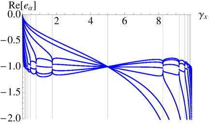
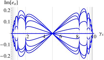
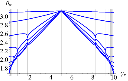
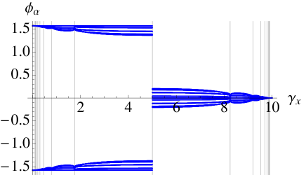
Figure 1: (Color online) Ground state real and imaginary parts (first and second panels) of pairing energies and polar and azimuthal angles of zeros (third and fourth panels) of the phase-space probability distribution $Q_{\psi}$ representing the ground state, for $j=10$, associated to the trajectory $\gamma_{x}=-\gamma_{y}+10$ for $0<\gamma_{x}<10$. The values of $\gamma_{x}$ where pairing energies or zeros degenerate are indicated by grey vertical lines.

Multiplicity of zeros and degeneracy of pairing energies.- Additionally one can appreciate the presence of collapses (vertical grey lines in Fig. 1) for certain values of the parameter $\gamma_{x}$ of the LMG Hamiltonian. These collapses or places where several zeros of the Husimi function or pairing energies join are determined by the expression

$$\gamma_{x}=5\pm\sqrt{5^{2}-\left(\frac{2j-1}{2j-1-2k}\right)^{2}}\,,k=0,...,j-1\,,$$ (11)

for the trajectory $\gamma_{x}=-\gamma_{y}+10$. This expression is obtained at the intersections between the straigthline $\gamma_{x}=-\gamma_{y}+10$ and the family of hyperbolas $\gamma_{x}\gamma_{y}=[({2j-1})/({2j-1-2k})]^{2}$ with $k=0,...,j-1$. Notice that the point $\gamma_{x}$ given in (11) must be real and then it exists if $k\leq\lfloor 2/5(2j-1)\rfloor$. The symbol $\lfloor x\rfloor$ means the smallest integer part of $x$. This family of points $(\gamma_{x},\gamma_{y}=5)$ has the property that each element verifies that the ground state amplitude of the Husimi function, $\langle\zeta|\psi\rangle$, has $j-k$ different zeros, one of them of multiplicity $2(k+1)$ and the others $j-k-1$ of multiplicity $2$. Therefore when the path $\gamma_{x}=-\gamma_{y}+10$, crosses each point of the above family, the zeros of the ground state $Q_{\psi}$ function join with the aforementioned multiplicity. We want to stress that due to the relation given in Eq. (9) the same behavior is displayed by the pairing energies. For the trajectory $\gamma_{x}=\gamma_{y}$ with $\gamma_{x}>-1$, one verifies that the ground state Husimi function has only one zero (the north pole in the Riemann sphere) of multiplicity $2j$, so that all the zeros of the $Q_{\psi}$ function (and thus all the pairing energies) join at the point $\gamma_{x}=\gamma_{y}=5$. The coefficients appearing in the family of hyperbolas, that is $-({2j-1})/({2j-1-2k})$, define the $\gamma_{x}$ values where there are crossings between the even and odd energy levels, when one takes $\gamma_{x}=\gamma_{y}$ (these points are explicitly calculated in octavio2005 ). Concerning the physical interpretation of the pairons’ collapses, there are several analysis in the literature, for example in the context of the SU(2) Richardson-Gaudin exact solution of a gas of spinless fermions collapses . In this context, pairons’ collapses are representing bound pairs because the pairons are real and negative. In our case, as it can be seen in Figure 1, all the particles form bound pairs at the point $\gamma_{x}=5$, while at the right- and left-hand sides of $\gamma_{x}=5$ the number of bound pairs decreases and the number of dispersion states increases. Notice that for $\gamma_{x}=0$ all the Cooper pairs are deconfined (in the sense of Ref. collapses ).

Experimental setups for state reconstruction and the determination of zeros and pairing energies.- Concerning the physical meaning and the experimental determination of the zeros of $Q_{\psi}$ for a spin system like LMG, let us discuss two possible experimental setups. The first one is related to the fact that the coherent state $|\zeta\rangle$ is the rotation of $|j,-j\rangle$ about the axis $\vec{r}=(\sin\phi,-\cos\phi,0)$ in the $x$-$y$ plane by an angle $\theta$, that is $|\zeta\rangle=\exp(-i\theta\vec{r}\cdot\vec{J})|j,-j\rangle$. A possible procedure for quantum-state reconstruction is explained in References Amiet ; Mann . Basically, the phase-space distribution $Q_{\psi}(\zeta)=|\langle\zeta|\psi\rangle|^{2}$ is precisely the probability to measure $m=-j$ in $\psi$, which can be determined by means of, for example, a Stern-Gerlach apparatus oriented along $\vec{R}(\theta,\phi)=(\sin\theta\cos\phi,\sin\theta\sin\phi,\cos\theta)$ (see e.g. Ref. Amiet ). Repeting this procedure (with a large number of identically prepared systems) for a finite number of orientations $(\theta,\phi)$, one can determine the function $Q_{\psi}$ and, therefore, its zeros. Actually, the zeros $\zeta_{0}$ of $Q_{\psi}$ are just those orientations $\vec{R}(\theta_{0},\phi_{0})\leftrightarrow\zeta(\theta_{0},\phi_{0})$ of the Stern-Gerlach apparatus for which the probability of the outcome $m=-j$ vanishes. Simulations of the LMG model in a Bose-Einstein condensate in a double-well potential are known (see e.g. Chen ). In this context, the polar angle $\theta$ is related to the population imbalance $j\cos\theta$ (the mean value of $J_{z}$), and the azimuthal angle $\phi$ is the relative phase of the two spatially separated Bose-Einstein condensates. Both quantities can be determined in terms of matter wave interference experiments as is shown in Refs. prl92 ; prl95 ; science307 .

Therefore, the reconstruction of any state $|\psi\rangle$ and the possibility to measure pairing energies in terms of the zeros of $Q_{\psi}$ are then experimentally accessible.

Extension to other bosonic BCS-like models.- The correspondence between pairing energies and zeros of the probability distribution representing a state in phase space is also present in other higher-dimensional BCS models, although the relation is a little bit more subtle. Let us consider for example the bosonic counterpart of (1), where $c_{k\sigma}$ are now boson $b_{k\sigma}$ annihilation operators. We shall consider $L+1$ scalar bosons $b_{0},b_{1},\dots,b_{L}$. In the case of uniform couplings $\gamma_{kkll^{\prime}}=\gamma/4$, the complete set of eigenstates of this model is given by

$$|\psi_{M,\nu}\rangle=\displaystyle\prod_{\alpha=1}^{M}\left(\sum_{\ell=0}^{L}\frac{b_{\ell}^{{\dagger}}b_{\ell}^{{\dagger}}}{2\varepsilon_{\ell}-e_{\alpha}}\right)|\nu\rangle,$$ (12)

where $|\nu\rangle=|\nu_{0},\dots,\nu_{L}\rangle$ is a state of $\nu=\sum_{\ell=0}^{L}\nu_{\ell}$ unpaired bosons and $\nu_{\ell}=0,1$ are the seniorities. The total number of particles is $N=2M+\nu$, with $M$ the number of paired bosons. As for the LMG model, each eigenstate $|\psi_{M,\nu}\rangle$ is completely determined by a set of $M$ pairing energies $e_{\alpha}$ (which are solutions of a set of coupled non-linear Richardson’s equations dukelskinp05 ) and their energies are given by $E_{M,\nu}(e)=\sum_{\ell=0}^{L}\varepsilon_{\ell}\nu_{\ell}+\sum_{\alpha=1}^{M}e_{\alpha}$. The $Q_{\psi}$ probability distribution of any quantum state $\psi$ for this model is the squared modulus of the overlap between $|\psi\rangle$ and a general $SU(L+1)$ coherent state

$$|\zeta\rangle=\frac{1}{\sqrt{N!}}\frac{(b_{0}^{\dagger}+\sum_{\ell=1}^{L}\zeta_{\ell}b^{{\dagger}}_{\ell})^{N}}{(1+\sum_{\ell=1}^{L}|\zeta_{\ell}|^{2})^{N/2}}|0\rangle,$$ (13)

which is a generalization of (7) for $\zeta=(\zeta_{1},\dots,\zeta_{L})\in\mathbb{C}^{L}$. The $Q_{\psi}$ amplitude of an eigenstate (12) turns out to be

$$\langle\psi_{M,\nu}|\zeta\rangle = \frac{\sqrt{N!}\prod_{\ell=1}^{L}\zeta_{\ell}^{\nu_{\ell}}}{(1+\sum_{\ell=1}^{L}|\zeta_{\ell}|^{2})^{N/2}}$$

$$\times\displaystyle\prod_{\alpha=1}^{M}\left(\frac{1}{2\varepsilon_{0}-\bar{e}_{\alpha}}+\sum_{\ell=1}^{L}\frac{\zeta_{\ell}^{2}}{2\varepsilon_{\ell}-\bar{e}_{\alpha}}\right).$$

Therefore, the zeros $\zeta_{\ell,\alpha},\alpha=1,\dots,M$ of $\langle\psi_{M,\nu}|\zeta\rangle$ lie now on $L$-dimensional complex ellipsoids

$$\frac{\zeta_{1,\alpha}^{2}}{\xi_{1,\alpha}^{2}}+\dots+\frac{\zeta_{L,\alpha}^{2}}{\xi_{L,\alpha}^{2}}=1,\;\;\xi_{\ell,\alpha}^{2}=\frac{2\varepsilon_{\ell}-\bar{e}_{\alpha}}{\bar{e}_{\alpha}-2\varepsilon_{0}},$$ (15)

with semi-principal axes of complex “length” $\xi_{\ell,\alpha}$. Still, there is a correspondence between pairing energies and complex ellipsoids in phase space, where the $Q_{\psi}$ distribution vanishes. Moreover, the occurrence (or absence) of $\zeta_{\ell}=0$ as a zero of (Searching for pairing energies in phase space) means seniority $\nu_{\ell}=1$ (or $\nu_{\ell}=0$).

Conclusions.- Exploiting the exact solvability of the LMG model (as a particular case of $SU(1,1)$ Richardson-Gaudin integrable model), we have revealed an interesting relation between pairing energies and zeros of a phase space probability distribution representing the quantum state in finite-size pairing mean-field like models. Zeros are experimentally accessible and this gives a method to find pairing energies’ multiplicities across the control parameter space. As a byproduct, knowing the zeros, one can reconstruct the corresponding state. These results are proven to be valid for a large class of paring systems and, in principle, they could be extended to other systems where particles pairs emerge.

References

- (1) S. Fujita, S. Godoy, Quantum Statistical Theory of Superconductivity, Kluwer Academic Publishers, Hingham, MA, USA (1996).
- (2) A. Bohr, B.R. Mottelson, D. Pines, Phys. Rev. 110 936 (1958).
- (3) H. J. Lipkin, N. Meshkov, and A. J. Glick, Nucl. Phys. 62, 188 (1965); 62, 199 (1965); 62, 211 (1965).
- (4) F. Pan, J.P. Draayer Phys. Lett. B 451, 1 (1999).
- (5) M. Kitagawa and M. Ueda, Phys. Rev. A 47, 5138 (1993); S. Dusuel and J. Vidal, Phys. Rev. Lett. 93, 237204 (2004).
- (6) G.J. Milburn, J. Corney, E.W. Wright, D.F. Walls, Phys. Rev. A 55, 4318 (1997); A.J. Leggett, Rev. Mod. Phys. 73, 307356 (2001); A. Micheli, D. Jaksch, J.I. Cirac, P. Zoller, Phys. Rev. A 67, 013607 (2003).
- (7) J. Dukelsky and P. Schuck, Phys. Rev. Lett. 86, 4207 (2001).
- (8) J. Dukelsky, C. Esebbag, and P. Schuck, Phys. Rev. Lett. 87, 066403 (2001).
- (9) G. Ortiz , R. Somma , J. Dukelsky, S. Rombouts, Nucl. Phys. B 707 [FS] 421 (2005).
- (10) J. Dukelsky and S. Pittel, Phys. Rev. Lett. 86, 4791 (2001).
- (11) P. Leboeuf and A. Voros, J. Phys. A 23, 1765 (1990).
- (12) G. Kirchmari et al., Nature 495, 205 (2013).
- (13) F. J. Arranz, Z. S. Safi, R. M. Benito, and F. Borondo, Eur. Phys. J. D 60, 279 (2010).
- (14) P. A. Dando and T. S. Monteiro, J. Phys. B 27, 2681 (1994).
- (15) J. M. Tualle and A. Voros, Chaos Solitons Fractals 5 1085 (1995)
- (16) D. Weinmann, S. Kohler, G-L. Ingold, and P. Hanggi, Ann. Phys. (Lpz) 8 SI277 (1999).
- (17) F. J. Arranz et al. Phys. Rev. E 87, 062901 (2013).
- (18) I. Bengtsson and K. Zyczkowski, Geometry of Quantum States: An introduction to Quantum Entanglement, Cambridge University Press, 2006.
- (19) S. Chaudhury, A. Smith, B. E. Anderson, S. Ghose and P. S. Jessen, Nature 461, 768 (2009)
- (20) C. Aulbach, A. Wobst, G.-L. Ingold, P. Hanggi and I. Varga, New J. Phys. 6, 70 (2004).
- (21) E. Romera, R. del Real and M. Calixto, Phys. Rev. A 85, 053831 (2012); M. Calixto, R. del Real and E. Romera, Phys. Rev. A 86, 032508 (2012); E. Romera, M. Calixto and O. Castaños, Phys. Scr. 89, 095103 (2014).
- (22) P. Ribeiro, J. Vidal and R. Mosseri, Phys. Rev. Lett. 99, 050402 (2007).
- (23) P. Ribeiro, J. Vidal and R. Mosseri, Phys. Rev. E 78, 021106 (2008).
- (24) P.W. Anderson, Phys. Rev. 112, 1900 (1958).
- (25) S. Lerma, J. Dukelsky, Nuclear Physics B 870, 421 (2013).
- (26) E. Majorana, Nuovo Cimento 9, 43-50 (1932).
- (27) O. Castaños, R. López-Peña, J. G. Hirsch, and E. López-Moreno, Phys. Rev. B 72, 012406 (2005).
- (28) S. M. A. Rombouts, J. Dukelsky and G. Ortiz, Phys. Rev. B 82, 224510 (2010).
- (29) J.-P. Amiet and S. Weigert, J. Opt. B: Quantum Semiclass. Opt. 1, L5-L8 (1999).
- (30) C Brif and A Mann, J. Opt. B: Quantum Semiclass. Opt. 2, 245-251 (2000)
- (31) G. Chen, J. -Q. Liang and S. Jia, Optics Express 17, 19682 (2009).
- (32) Y. Shin, M. Saba, T.A. Pasquini, W. Ketterle, D.E. Pritchard and A.E. Leanhard, Phys. Rev. Lett. 92, 050405 (2004).
- (33) M. Albeitz, R. Gati, J. Folling, S. Hunsmann, M. Cristiani, and M.K. Oberthaler, Phys. Rev. Lett 95, 010402 (2005).
- (34) M. Saba, T.A. Pasquini, C. Sanner, Y. Shin, W. Ketterle, and D.E. Pritchard, Science 307, 1945 (2005)