The red sequence of Abell X-ray underluminous clusters

Abstract

We present an analysis of the colour-magnitude relation for a sample of 56 X-ray underluminous Abell clusters, aiming to unveil properties that may elucidate the evolutionary stages of the galaxy populations that compose such systems. To do so, we compared the parameters of their colour-magnitude relations with the ones found for another sample of 50 “normal” X-ray emitting Abell clusters, both selected in an objective way. The $g$ and $r$ magnitudes from the SDSS-DR7 were used for constructing the colour-magnitude relations. We found that both samples show the same trend: the red sequence slopes change with redshift, but the slopes for X-ray underluminous clusters are always flatter than those for the normal clusters, by a difference of about 69% along the surveyed redshift range of 0.05 $\leq z<$ 0.20. Also, the intrinsic scatter of the colour-magnitude relation was found to grow with redshift for both samples but, for the X-ray underluminous clusters, this is systematically larger by about 28%. By applying the Cramér test to the result of this comparison between X-ray normal and underluminous cluster samples, we get probabilities of 92% and 99% that the red sequence slope and intrinsic scatter distributions, respectively, differ, in the sense that X-ray underluminous clusters red sequences show flatter slopes and higher scatters in their relations. No significant differences in the distributions of red-sequence median colours are found between the two cluster samples. This points to X-ray underluminous clusters being younger systems than normal clusters, possibly in the process of accreting groups of galaxies, individual galaxies and gas.

1 Introduction

Since Baum (1959) noticed that, within a sample of elliptical galaxies, the brightest are generally the reddest ones, several studies have demostrated that the red galaxy population traces a straight line in colour-magnitude diagrams, with a well-defined slope and small scatter ($\leq$ 0.1 mag; e.g. Visvanathan & Sandage, 1977; Bower et al., 1992b; van Dokkum et al., 1998; Andreon, 2003; López-Cruz et al., 2004; McIntosh et al., 2005). This makes the colour-magnitude relation (CMR) a useful tool for getting information about the formation and evolution of galaxy cluster members.

The CMR can be used for estimating the redshift of a cluster when photometry in at least two bands is available (e.g. Visvanathan & Sandage, 1977; Bower et al., 1992b; Andreon, 2003; López-Cruz et al., 2004), while a blind search for CMRs may be used for finding galaxy overdensities associated to galaxy clusters (e.g. Gladders & Yee, 2000). The slope of the CMR has been interpreted as a consequence of the mass-metallicity relation: more massive (or luminous) galaxies have redder colours (e.g. Faber, 1973; Arimoto & Yoshii, 1987; Kodama & Arimoto, 1997). The mass-metallicity relation, on the other hand, is thought to be originated from the tendency of galaxies to lose their metals due to galactic winds, the loss being more pronounced for galaxies with shallower potential wells or lower masses (e.g. Arimoto & Yoshii, 1987; Kodama et al., 1998; van Dokkum et al., 2001; Tremonti et al., 2004; Gallazzi et al., 2006). An alternative model (Kauffmann & Charlot, 1998) considers the effect of the formation of elliptical galaxies by the merging of disk systems: the mass-metallicity relation would be already established for the progenitors, and the more massive ellipticals are formed from more massive disks. Other works have shown that the CMR depends neither on cluster/group richness (Andreon, 2003) nor on the environment (Hogg et al., 2004), but luminous galaxies are more abundant in higher over-density regions and blue galaxies reside towards the outskirts of the clusters (McIntosh et al., 2005; Hogg et al., 2004), a reminiscence of the morphology-density relation (e.g. Dressler, 1980).

The physical interpretation of these relations and properties is not fully understood. The CMR tight scatter has been interpreted as evidence that galaxies residing in this sequence are coeval, with a small spread in their formation age, which mostly occurred at $z\,\geq\,$2.0 and evolved passively since then (e.g. Bower et al., 1992b, 1997, 1998; Lubin, 1996; Ellis et al., 1997; Gladders et al., 1998; Kodama et al., 1998; van Dokkum et al., 1998; Andreon, 2003; McIntosh et al., 2005). Other works have suggested that the age of the galaxies could drive the CMR (e.g. Ferreras et al., 1999; Terlevich et al., 1999; Trager et al., 2000). Some studies, like Skelton et al. (2009) and Jiménez et al. (2011), have considered the effect of gas-poor mergers on the CMR with a toy model, concluding that the relation changes its slope at the bright end and becomes bluer and with lower scatter. It is worth mentioning that, besides ellipticals, lenticulars and passive spirals also populate the CMR (e.g. Bamford et al., 2009; Masters et al., 2010; Sodré, Ribeiro da Silva & Santos, 2013).

On the other hand, the majority of galaxy clusters have most of their baryons in the form of a hot, diffuse plasma, that may interact with the colder interstellar gas (interstellar medium) due mainly to the motion of galaxies inside clusters. The ram-pressure effect (Gunn & Gott, 1972; Larson et al., 1980), i.e. the hydrodynamical interaction between the intracluster medium (ICM) and the interstellar medium, may strip the gas of the galaxies, quenching star formation or even enhancing it while the gas is being compressed, affecting galaxy evolution and hence the colours of cluster galaxies (Fujita & Nagashima, 1999; Weinberg, 2013).

The ICM properties, such as luminosity and temperature, are observed to scale with the mass of the cluster, but possibly not in a self-similar manner, as described by the scaling relations between X-ray luminosity or temperature and virial mass ($L_{\mathrm{X}}$-$M_{\mathrm{v}}$ and $T_{\mathrm{X}}$-$M_{\mathrm{v}}$, e.g. Reiprich & Böhringer, 2002; Rykoff et al., 2008), and X-ray temperature with galaxy velocity dispersion ($T_{\mathrm{X}}$-$\sigma$, e.g. Lubin & Bahcall, 1993; Xue & Wu, 2000).

In recent years, several studies have found galaxy systems with most properties of galaxy clusters but underluminous in X-rays (Bower et al., 1997; Lubin et al., 2004; Dietrich et al., 2009), with respect to the scaling relations mentioned above. Dynamical analyses of these systems suggest that they are young systems still undergoing a phase of gas accretion and/or merging of smaller groups and galaxies; that is, they may not have yet reached the virial equilibrium. Other works, however, debate the very existence of these objects (e.g., Andreon & Moretti, 2011).

Our objective with the present work is to investigate the properties of the CMR of X-ray Underluminous Abell clusters (AXUs, following Popesso et al., 2007 naming) in comparison with “Normal” X-ray emitting Abell clusters (AXNs) to verify whether the ICM is indeed important in shaping up the red sequence. The paper is organized as follows: the optical and X-ray data are described in §2. The identification of the red sequence, its analysis and comparisons between samples are presented in §3. Our main results are summarized in §4 and final comments and conclusions in §5 and §6, respectively.

We will assume a $\Lambda$CDM cosmology with $\Omega_{m}=$ 0.30, $\Omega_{\Lambda}=$ 0.70 and $H_{0}=$ 70 km s^-1 Mpc^-1 throughout the paper.

2 Data

The analysis presented in this paper is based on a comparison of the CMR properties between a sample of AXUs and a sample of AXNs. The colour data for both samples were extracted from the Sloan Digitized Sky Survey, Data Release 7 (SDSS-DR7, Abazajian et al., 2009).

The sample of AXUs comes from that of the optically selected clusters by Popesso et al. (2007, hereafter P07); their original sample was defined from the Abell (1958) cluster catalog in the region covered by Sloan Digitized Sky Survey, Data Release 3 (SDSS-DR3, York et al. 2000). That sample contains 137 spectroscopically confirmed clusters, 51 of which were only marginally detected (between $2$ and $3\sigma$) in the ROSAT All Sky Survey data (RASS, Voges et al. 1999) or presenting no clear X-ray emission (detection level $\sim\,1\sigma$). The authors determined X-ray luminosities and virial masses in order to analyze the $L_{\mathrm{X}}$-$M_{200}$ relation. They classified these 51 clusters as AXU clusters based on the poorly detected or undetected signal of X-ray emission and the fact that, on average, these did not follow the $L_{\mathrm{X}}$-$M_{200}$ scaling relation. However, since the first criterion is subject to debate, because it is not clear if significant X-ray emission may be necessarily expected for all the clusters in the sample (mainly due to the shallow depth of the RASS), and the second is only a statistical one, we applied an independent criterion to separate the AXU clusters. We analyzed the $L_{\mathrm{X}}$-$M_{200}$ relation for the optically selected clusters of P07 and defined as AXUs the clusters (56 systems) with $\Delta\log{\mathrm{L_{X}}}\leq-0.75$, where the $\Delta\log{\mathrm{L_{X}}}$ is the difference between the calculated and predicted cluster X-ray luminosity (Figure 1), according to the same scaling relation presented in P07. There is no clear argument for using this threshold for separating the AXU clusters. Since this sample contains both AXUs and AXNs, we only require that the AXUs have the most negative values of $\Delta\log{\mathrm{L_{X}}}$. However, the P07 scaling relation was obtained for AXN clusters only (in fact the same sample we use in the present paper, to be described below) and the original fit has a standard deviation of 0.43 in $\Delta\log{\mathrm{L_{X}}}$, which means that our separating line is roughly about 2$\sigma$ from the scaling relation (that is, 92% of the AXNs should be excluded by applying this threshold), making us confident that we are close to selecting a bona fide AXU’s population.

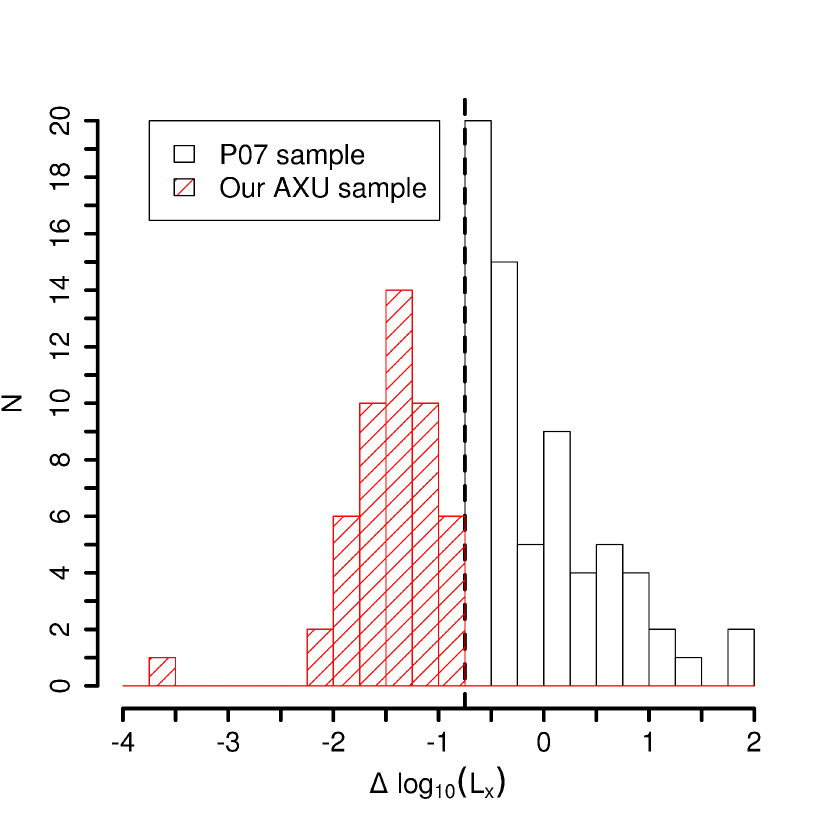
Figure 1: Distribution of the residuals for P07 sample, defined as the difference between measured and predicted (by the scaling relation for AXNs) cluster X-ray luminosity ($\Delta\log_{10}{\mathrm{L_{X}}}\,=\,\log_{10}\mathrm{L_{X,m}}-\log_{10}\mathrm{L_{X,p}}$). All clusters below $\Delta\log_{10}{\mathrm{L_{X}}}\leq-0.75$ (hatched histogram) are considered as our AXU sample.

In addition, P07 also present an estimate of the number of cluster members (within 1 Abell radius), redshift ($z$), velocity dispersion ($\sigma_{v}$), cluster virial radius ($r_{200}$), d1 probability that the cluster does not contain substructures (P_DS), and an X-ray class (a classification based on the quality of the X-ray detection). For such AXU sample, we extracted position and photometric data (in the $g$ and $r$ bands, corrected for extinction from GALAXY and DERED tables, Strauss et al. 2002) from SDSS-DR7 for galaxies brighter than $r\,=\,22$ within a projected $r_{200}$ radius of each cluster centre (taken directly from P07). Figure 2 shows some general properties of the AXU sample (shaded histograms). The median (mean) values of some properties of these clusters are presented in Table 1.

Table 1. General properties: median (mean) values
Sample	$r_{200}$	$z$	$M_{200}$	$L_{\mathrm{X}}$
	$h^{-1}$Mpc		10${}^{14}\,h^{-1}$M⊙	10${}^{44}\,h^{-2}$ergs s-1
AXU	1.08 (1.10)	0.106 (0.106)	2.90 (3.59)	0.03 (0.05)
AXN	0.98 (1.00)	0.113 (0.111)	2.67 (3.02)	1.29 (1.90)

Table 1: General properties of the AXN and AXU samples. Note that, although the median (mean) mass of AXU clusters is slightly higher, their luminosties are significantly lower.

Our comparison sample comes from the list of 114 “normal” X-ray emitting clusters described in Popesso et al. (2004, hereafter P04). This sample was analyzed in the same way as the AXU sample and has 91 galaxy clusters with $M_{200}$ and $r_{200}$ information from Piffaretti et al. (2011), but only 50 are in the same redshift range of our AXU sample, and they will be our AXN sample. Figure 2 also shows the properties of the AXN sample (solid line histograms). The median (mean) values of these properties are also presented in Table 1.

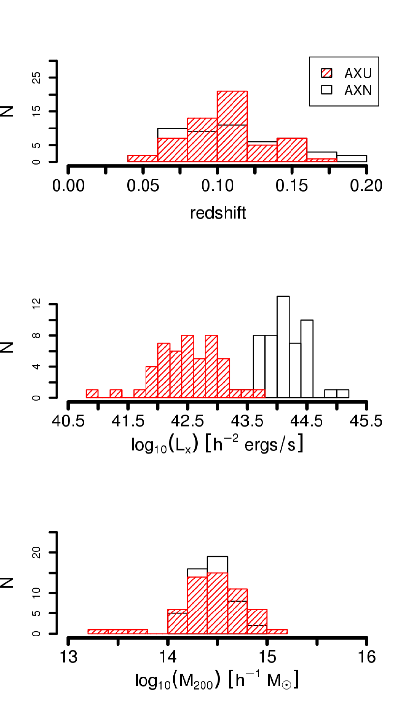
Figure 2: General properties for the sample of 56 AXUs (hatched histograms) and 50 AXNs (solid line histograms).

From now on, we will divide the samples in 5 redshift bins (details below). In Figure 3 we test if our division in bins is sufficiently homogeneous for properly comparing the red sequence fits. We can see that the median mass is almost the same for all bins (0.075$\,<\,z\,<\,$0.200), except for the first bin, being slightly displaced in the sense that the clusters in our AXU sample are in general more massive than AXNs. We believe this does not affect significantly our results since most of the signal is in the three intermediate bins. On the other hand, this may point out that AXU clusters, being possibly younger systems, are not necessarily less massive (they may still be currently accreting clumps of galaxies and increasing their masses) or could have their masses overestimated due to their unrelaxed dynamical state.

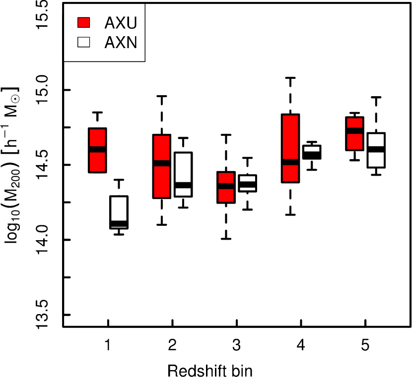
Figure 3: Boxplots of the median mass comparison between AXUs and AXNs in the different redshift bins considered for CMR analyses. The filled boxes (red in the electronic version) are the AXU cluster mass range and the white ones are the AXNs. The black thick lines inside boxes are the median mass values while the large boxes are the inter-quartile ranges (defined as the difference between the third and first quartiles) of the mass distribution. Also, the “error bars” are the first and third quartile minus 1.5 times the inter-quartile range.

3 Analysis

A rest-frame analysis of the CMR of a sample covering a range in redshifts requires k-correction of galaxy magnitudes. Since the k-correction depends also on the SED of the galaxy (usually approximated, for practical purposes, by using a colour index or morphological class), some artificially large spread may be expected, especially at higher redshifts, due to the uncertainties in the SED proxy parameters. Thus, despite the fact that there are recent useful k-correction estimations for SDSS-DR7 galaxies (e.g. O’Mill et al., 2011), we decided to adopt a more robust approach, by comparing the CMR parameters in different redshift bins, with no k-corrections applied.

We divided our samples in five sub-samples comprising clusters within bins of 0.025 in redshift (except for the farthest one): 0.05$\,\leq\,z\,<\,$0.075, 0.075$\,\leq\,z\,<\,$0.10, 0.10$\,\leq\,z\,<\,$0.125, 0.125$\,\leq\,z\,<\,$0.15 and 0.15$\,\leq\,z\,<\,$0.20. The cluster galaxies (without k-correction), in each redshift bin, were stacked in the corresponding sub-sample. We, then, constructed density plots using a Gaussian kernel taking the peak value of the distribution as the centre of the red sequence (we also tested Epanechnikov, rectangular and biweight kernels, with the same peak value as result) and the bandwidth as the standard deviation of the kernel. Then, the limits for the colour range inside which the CMR was fitted were defined as $\pm$0.30 from the peak value. For the luminosity intervals, we have considered as the brigthest limit one magnitude brighter than the mean $r$ magnitude of the BCGs in the MaxBCG catalogue (Koester et al. 2007) in the same redshift bin, $\left\langle r_{BCG}\right\rangle-1$, and as the faintest limit $\left\langle\,r_{BCG}\right\rangle+4$, a reliable limit taking into account the SDSS completeness (e.g. Yasuda et al., 2001). Although the limits adopted for the present work were those just described (listed in Table 2 for each redshift bin), we also made two other tests: for the first one, we considered as the upper limit in $r$ magnitude $\left\langle r_{BCG}\right\rangle+5$ and, for the second one, we took as the lower limit in $r$ magnitude one magnitude brighter than the mean $\left\langle M_{r}^{*}\right\rangle$, using the Schechter parameters from Popesso et al. (2005), in the same redshift bin, converted to apparent magnitude, and as the upper limit $\left\langle M_{r}^{*}\right\rangle+4$, obtaining, for both alternative selections, similar results.

Table 2. Adoppted limits for red sequence fit per redshift bin
Redshift bin	Magnitude range	Galaxies in AXUs	Galaxies in AXNs
0.050$\,\leq\,z\,<\,$0.075	13.52-18.52	27865	18029
0.075$\,\leq\,z\,<\,$0.100	14.28-19.28	41449	24441
0.100$\,\leq\,z\,<\,$0.125	14.99-19.99	24963	10202
0.125$\,\leq\,z\,<\,$0.150	15.56-20.56	10028	7612
0.150$\,\leq\,z\,<\,$0.200	16.19-21.19	4552	4919

Table 2: Luminosity limits for the selection of red sequence galaxies in bins of redshift for the AXU and AXN samples. The lower and upper magnitude limits are $\left\langle r_{BCG}\right\rangle-1$ and $\left\langle r_{BCG}\right\rangle+4$, respectively. We show the number of galaxies, in the field, used for the analysis in each sub-sample.

For retrieving the slope and intercept of the stacked CMRs, after the first definition of limits in colour and luminosity, we have made a robust regression, using the MM-estimator included in the MASS package (Venables & Ripley 2002) in R (fitting is done by iterated re-weighted least squares, IWLS, where standard deviation of the error term is not constant over all values of the predictor or explanatory variables). Then, we redefined the boundaries of the box taking lines parallel to the previous fit, with the upper and lower limits on $\pm$0.30. The same fitting procedure was then repeated. This selection is similar to other recent choices in the literature (e.g. De Lucia & Poggianti 2008; Laganá et al. 2009), but our results are not qualitatively sensitive to this particular choice of $\pm$0.30, as we will see later. From the new fit we obtained the slope, intercept, intrinsic scatter, median and mean colours (Figures 4 and 5). The solid line, in both figures, is the fit by the robust regression (MM-estimator) of the red sequence while the dashed lines are 1$\sigma$ error bars from the fit. The values in the boxes are: slope (a), intercept (b) and intrinsic scatter (s).

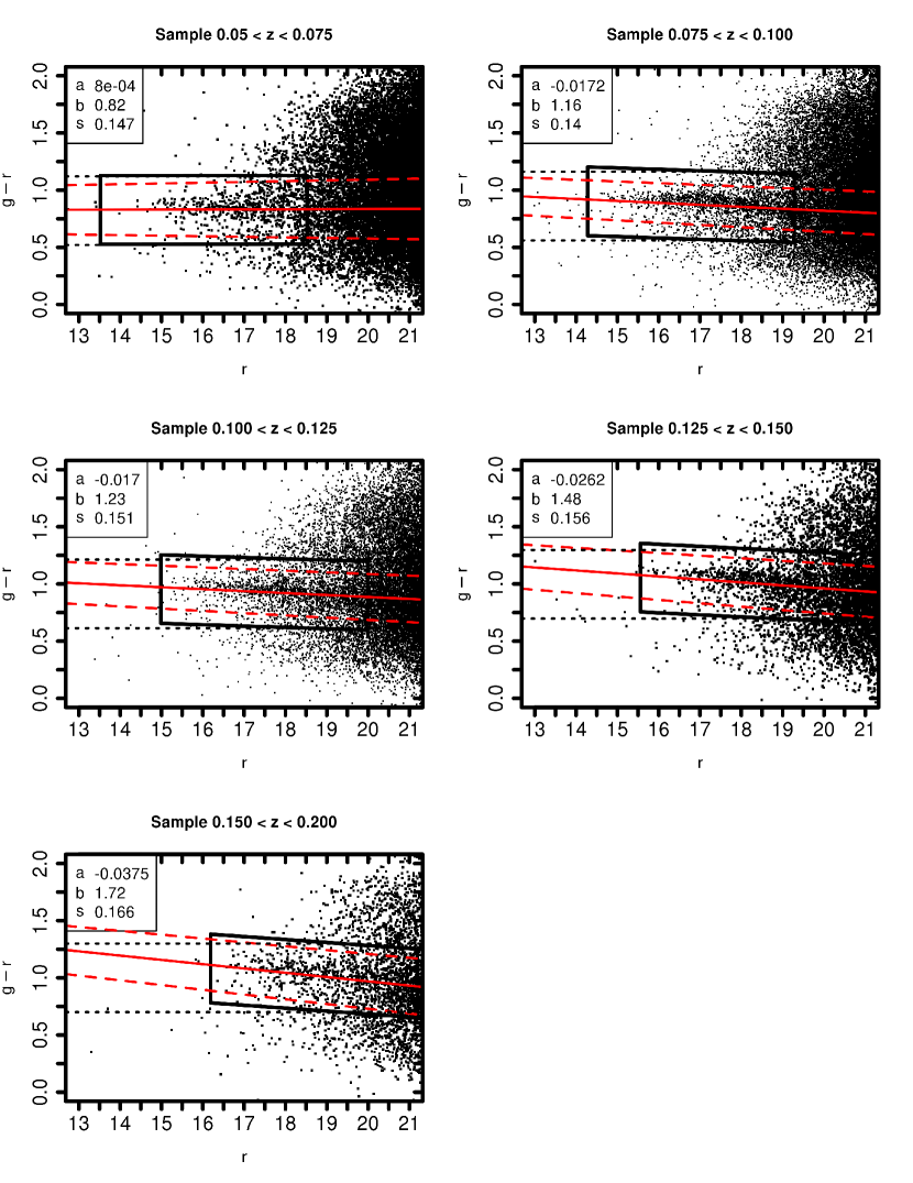
Figure 4: Colour-magnitude diagrams for each sub-sample of the AXU sample. The dotted lines are the first selection in colour and the solid rectangles (black in the electronic version) are the final red sequences selections. The solid lines are the regression fit and the dashed lines are 1$\sigma$ errors from fit (both red in the electronic version).

Table 3. Parameters of the red sequences
	AXU					AXN
Redshift bin	Slope	Intercept	Scatter	Colour		Slope	Intercept	Scatter	Colour
0.050$\,\leq\,z\,<\,$0.075	0.0008$\pm$0.0058	0.08$\pm$0.10	0.147	0.841$\pm$0.019		$-$0.0279$\pm$0.0029	1.29$\pm$0.05	0.082	0.822$\pm$0.037
0.075$\,\leq\,z\,<\,$0.100	$-$0.0172$\pm$0.0027	1.16$\pm$0.05	0.140	0.867$\pm$0.019		$-$0.0251$\pm$0.0019	1.31$\pm$0.03	0.089	0.865$\pm$0.012
0.100$\,\leq\,z\,<\,$0.125	$-$0.0170$\pm$0.0026	1.23$\pm$0.05	0.151	0.917$\pm$0.021		$-$0.0286$\pm$0.0027	1.46$\pm$0.05	0.109	0.938$\pm$0.015
0.125$\,\leq\,z\,<\,$0.150	$-$0.0262$\pm$0.0034	1.48$\pm$0.07	0.156	0.989$\pm$0.021		$-$0.0378$\pm$0.0026	1.69$\pm$0.05	0.120	0.983$\pm$0.016
0.150$\,\leq\,z\,<\,$0.200	$-$0.0375$\pm$0.0039	1.72$\pm$0.08	0.170	0.981$\pm$0.024		$-$0.0450$\pm$0.0029	1.95$\pm$0.06	0.146	1.075$\pm$0.020

Table 3: Parameters obtained after fitting the red sequences. For each sub-sample we get the slope, intercept, intrinsic scatter and median colour.

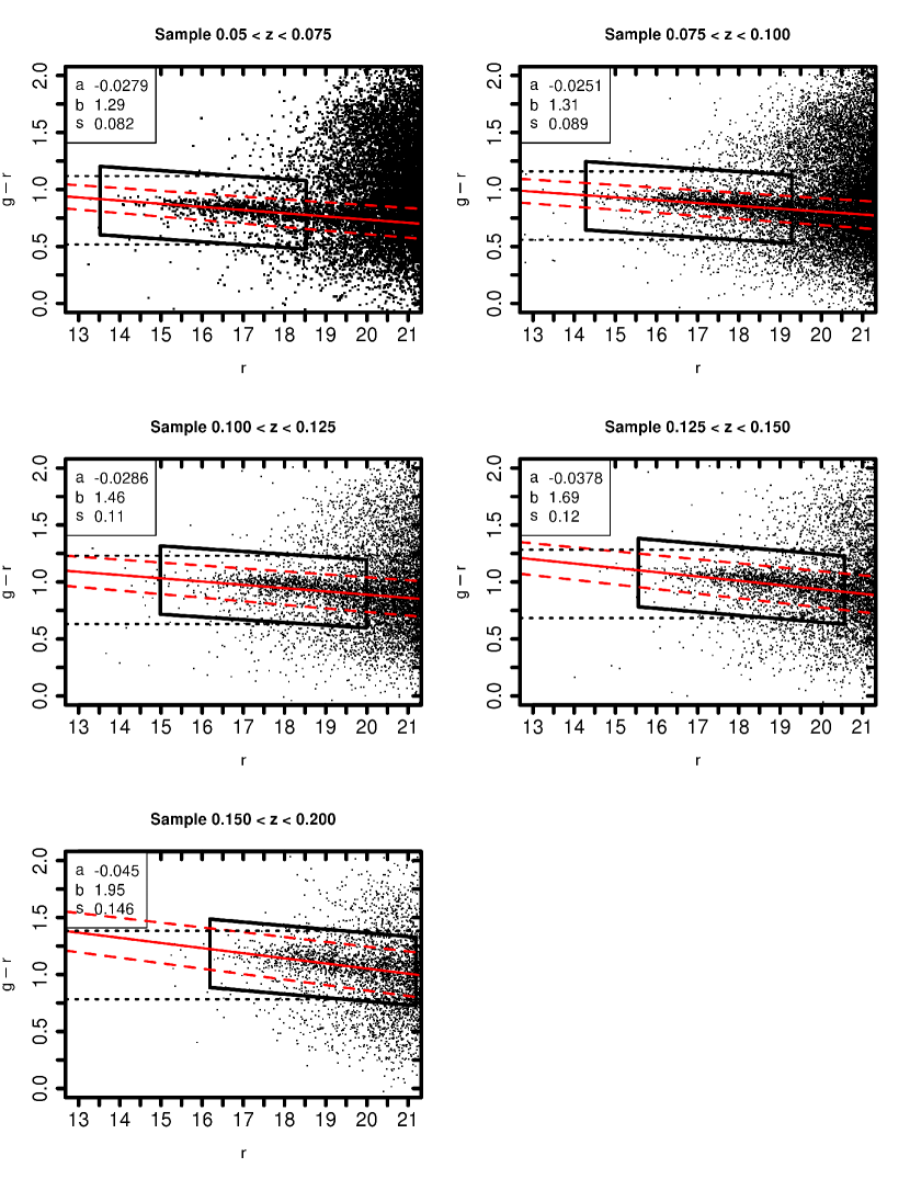
Figure 5: Colour-magnitude diagrams for each bin of redshift in the AXN sample.

4 Results

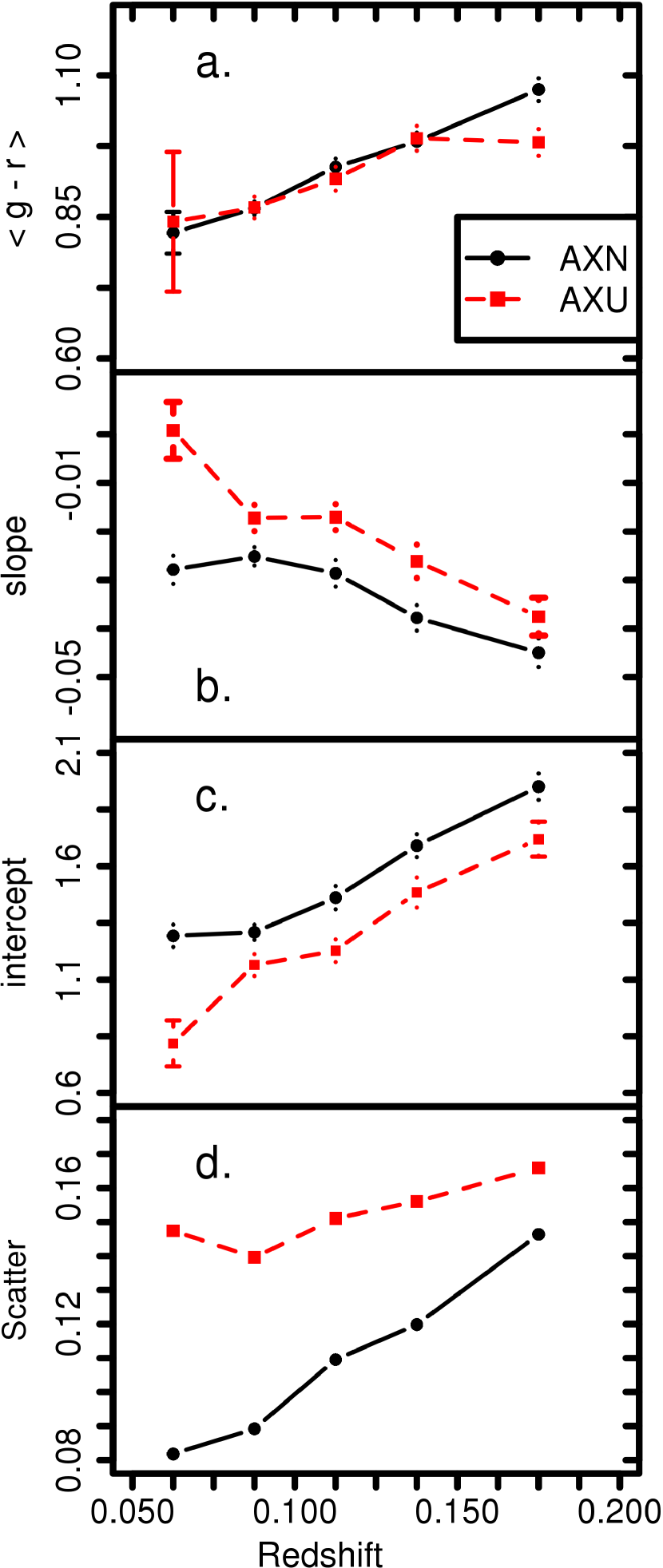
Figure 6: Results of the red sequence fitting for the two samples: AXN (closed squares and solid lines) and AXU (closed circles and dashed lines). Errors were obtained with the MM-estimator, except for the error of the median, which was obtained by bootstraping.

The results of the analysis explained in the previous section are presented in Table 3. Figure 6 shows that there are clear trends of CMR properties with redshift, in the sense that intercept, intrinsic scatter and median colour decrease with decreasing redshift. The slope seems to flatten with decreasing redshift.

The most obvious trend is the increase of the median colour with redshift (Figure 6, panel a), as expected since we did not apply any k-correction to these samples. Both AXN and AXU samples show consistently the same trend (with slightly larger dispersions for the last bin, probably because this bin is more subject to uncertainties due to the smaller numbers of AXU and AXN clusters there). This makes us confident that the samples are homogeneous at a first approximation and the techniques are adequate for the present study.

Other significant trends are the ones shown by the red sequence slope, which becomes flatter with decreasing redshift (panel b of Figure 6) and intercept, which consistently increases with redshift (panel c of Figure 6). Some previous works (Stanford et al., 1995, 1998; Santos et al., 2009; Mei et al., 2009) have suggested, based on high redshift cluster samples, that there seems to be no change in the slope of the CMR from $z\,=\,$1.3 to $z\,=\,0$. However, other authors have already found a similar trend at a similar redshift range as the one considered in the present work. López-Cruz et al. (2004) studied a sample of 57 Abell clusters of galaxies between 0.02 $\leq\,z\,\leq\,$0.18, selected by their X-ray emission. They show that their results are very well fitted by the models described by Kodama & Arimoto (1997), who concluded that the slope of the CMR is dominantly driven by a metallicity effect (instead of an age effect), taking its origin at early times probably from galactic wind feedback. The same conclusion was attained by Gladders et al. (1998), who studied a sample of clusters, with data from Hubble Space Telescope, reaching higher redshifts (up to 0.75).

More than confirming a change in the slope of the CMR with redshift, for both AXUs and AXNs, panel b of Figure 6 also reveals that the slopes of the two samples are intrinsically (and significantly) different. The CMR slopes for the AXUs are systematically flatter than the CMR slopes of the AXNs. The mean difference is about 0.014 (69%).

Our results on the intrinsic scatter of the CMR show an increase with redshift (Figure 6 panel d). This trend was also detected by van Dokkum (2002) who found that the scatter is larger at much higher redshifts (0.4$\,<\,z\,<\,$0.7), with a tendency to decrease after that (0.7$\,<\,z\,<\,$1.3). Again, both of our samples have a similar behavior, but with a noticeable zero point difference, in the sense that the AXU sample presents higher scatter by 0.043 (28%). Even considering that part of this effect could be produced by the increase in the photometric errors with redshift, about 15% along the studied redshift range, some significant difference (more than 20%) remains.

The fact that AXUs have probably less dense ICM may be related to their dynamical status, or, being more specific, to their assembling history, which should be expected since in an hierarchical collapse the gravitational compression of the gas may be slower than it would occur in a monolithic one. The point here is that this different dynamical status seems to be reflected in the evolutionary stage presented by the population of galaxies in clusters with “normal” (closer to relaxed) ICM or clusters with distinct intra-cluster characteristics. As far as we know there are no previous references to this behavior.

For estimating the significance of our results we applied the Cramér test (Baringhaus & Franz, 2004). For two distinct populations, this test estimates, in our case, the probability that de distribution of slope, intrinsic scatter and median colours differ between the samples (or more specifically we want to obtain the probability of rejecting the hypothesis that the values come from the same parent population, in each case).

In Table 4 we show the results for the Cramér test for the comparisons made in this work. We get a 92% probability that the distributions of slope, for the AXN and AXU samples, are different, 78% for the intercept, 99% for intrinsic scatter and 28% for the median colour. From these results we can conclude that for the slope and intrinsic scatter we get enough signal for a marginally significant difference between the two samples.

Table 4. Results of Cramér test
Sample	Slope	Intercept	Scatter	Colour
AXU $\times$ AXN	92%	78%	99%	28%

Table 4: Results obtained from applying the Cramér test to our AXU sample versus the AXN sample. The null hypothesis is that the compared samples come from the same parent population.

Finally, we made an additional test to evaluate if our results were dependent on the size of the selected box used to define the red sequence. In Figure 7 we show the resulting Cramér probabilities for the difference between the AXU and AXN samples analyzed for distinct box size selections (in colour limits). One can see that the results do not change when we decrease the limits to 0.2 and 0.15.

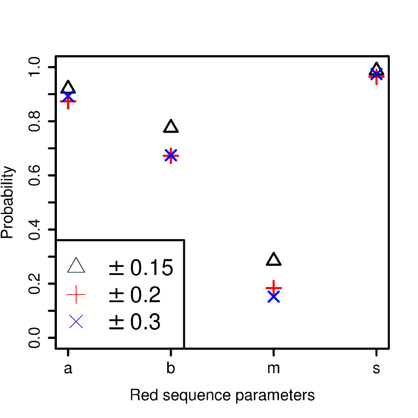
Figure 7: Results of the Cramér probability test for different colour range box sizes on fitting the red sequence. Slope (a), intercept (b), median colour (m) and intrinsic scatter (s).

5 Discussion

One usual interpretation of the slope of the CMR, as we mentioned before, relates to the redder colours of the most luminous galaxies due to their higher metallicities, directly associated to the mass-metallicity relation (e.g. Kodama & Arimoto, 1997; Kauffmann & Charlot, 1998). In this sense, a galaxy population presenting a CMR with steeper slopes should have, naively speaking, their most massive galaxies overabundant in metals (or their less massive galaxies being “submetallic”). In our samples, the steeper slopes of the red sequence on the CMRs are presented by the clusters with “normal” ICM, suggesting that the brightest galaxies in AXUs are less abundant in metals (or the faintest are more metallic). This is difficult to reconcile with the scenario where the metallicity of the ICM comes from the feedback of the member galaxies. In the assumption that the AXU clusters are still galaxy systems in the process of formation, their underluminosity suggest that their ICM did not reach virial equilibrium yet and, thus, they are probably also underdense (in gravitational systems, collapse makes the gas hotter except only for very high opacities). Since the ram pressure, as an important hydrodynamical effect that removes gas (and metals) from the galaxies, depends on gas density, an underdense ICM should produce less ram pressure. Thus, the galaxies in this environment should be more metallic, instead, specially the most massive ones. The correct scenario, thus, is probably much more complicated.

On the other hand, we can consider that the denser ICM (supposedly expected in a collapse closer to monolithic) may also produce more perturbation in the interestellar medium of the galaxies (by the same hydrodynamical effects) and will possibly stimulate the star formation in an initial phase (before it is sufficiently high to drag the cold gas and quench star formation). With more star formation, the galaxies produce more metals. In this sense, the metallicities of the galaxies are, on average, affected by the properties of the ICM (and also by their star formation histories). This could be correct if the most affected galaxies in this scenario were the most massive ones. The enhancement of star formation is expected to happen mainly in early epochs of the cluster evolution, what would explain the parallel relations (the clusters with less dense ICM would have flatter CMRs along all their lives). This scenario is also in agreement with the results by Tanaka et al. (2005) considering that the AXUs represent the lower density environments for which the CMR build-up is delayed.

Two questions remain open in this last scenario: the role of the feedback and typical metallicity of the ICM of underluminous clusters. We know that the metallicity of the AXNs is, on average, about 0.3 of the solar value, an already uncomfortably high value, but almost nothing is known about the metallicity of the AXU’s ICM.

Going into more detail, some recent models suggest that the fainter red-sequence (RS) galaxies have quenched their star formation only recently (and maybe suffered some events of wet mergers prior to that) and then settled in the RS (Smail et al., 1998; Tanaka et al., 2005; Faber et al., 2007; Miller et al., 2012). Brighter RS galaxies, instead, are the prototype RS galaxies: they had the bulk of their stellar content already in place at $z>$ 1 and only evolved by major or minor dry mergers (of other RS galaxies) after that. According to Jiménez et al. (2011), the effect of dry mergers is to increase the mass (and luminosity) of the galaxies without altering their metallicity (see, also, Bower et al., 1992b; Skelton et al., 2009). These authors suggest that the bright end of the CMR must have a flat slope. In this scenario, AXUs may have flattened their RS by a higher rate of dry mergers. The question that remains is how to relate these rates with the shallower ICM.

6 Conclusions

We compared the properties of the colour-magnitude relation, $(g-r)\times r$, of red galaxies in two samples: one with 56 X-ray underluminous clusters (from Popesso et al., 2007), and the other with 50 “normal” X-ray emitting clusters (from Popesso et al., 2004), in 5 bins of redshift. We have found that:

• Our results confirm previous findings that the slope of the CMR decreases with increasing redshift. Both samples show the same trend, but the slopes of AXUs are always flatter than the slopes of AXNs, by a difference of about 69% (0.014) along the surveyed redshift range.

• The intrinsic scatter of the CMR was found to grow with redshift, for both samples. Again, there is a zero point difference between the relations (intrinsic scatter $\times$ redshift) found for the AXUs and the AXNs, in the sense that the intrinsic scatter of the AXUs is systematically larger by more than 28% (0.043).

Our data allow an interpretation such as that galaxies evolve in a distinct way in different environments concerning the properties of the ICM, which may be a consequence of the different dynamical status of the systems, being subject to different levels of star formation stimulation and, consequently, having different levels of metallicities, specially the more massive galaxies. In an initial phase of structure formation, a denser ICM would be expected to enhance star formation in more massive galaxies, by exerting more hydrodynamical pressure. This scenario would lead the brightest galaxies in the AXN clusters to be more metallic than their counterparts of the AXU clusters and, consequently, generating distinct slopes in their CMRs. If the X-ray underluminous clusters are, as previously proposed, less dense galaxy systems, this scenario is in accordance with the one proposed by Tanaka et al. (2005), in which the CMR build-up for less dense clusters is delayed. The larger intrinsic scatter for AXUs is also in agreement with this scenario: a longer time for producing the CMR implies also a larger dispersion in formation ages. A higher rate of dry mergers in X-ray underluminous clusters would also possibly produce the different slopes, but it is difficult to explain such an excess of interaction.

This file has been amended to highlight the proper use of LaTeX 2εcode with the class file.

References

- Abazajian et al. (2009) Abazajian, K. N., Adelman-McCarthy, J. K., Agüeros, M. A., Allam, S. S., Allende Prieto, C., An, D., Anderson, K. S. J., Anderson, S. F., Annis, J., Bahcall, N. A., et al. 2009, ApJS, 182, 543.
- Abell (1958) Abell, G. O., 1958, ApJS, 3, 211.
- Andreon (2003) Andreon, S., A& A, 2003, 409, 37.
- Andreon & Moretti (2011) Andreon, S. & Moretti, A. arxiv 1109.4031.
- Arimoto & Yoshii (1987) Arimoto, N., Yoshii, Y., A&A, 173, 23.
- Bamford et al. (2009) Bamford, S. P., et al., 2009, MNRAS, 393, 1324.
- Baringhaus & Franz (2004) Baringhaus, L. and Franz, C., 2004, Journal of Multivariate Analysis, 88, 190.
- Baum (1959) Baum, W. A. 1959, PASP, 71, 106.
- Bower et al. (1992b) Bower, R. G., Lucey, J. R. & Ellis, R. S., 1992, MNRAS, 254, 601.
- Bower et al. (1997) Bower, R. G., Castander, F. J., Ellis, R. S., Couch, W. J., Böhringer, H. 1997, MNRAS, 291, 353.
- Bower et al. (1998) Bower, R. G., Kodama, T. & Terlevich, A., 1998, MNRAS, 299, 1193.
- De Lucia & Poggianti (2008) De Lucia, G. & Poggianti, B. M., 2008, ASPC, 399, 314.
- Dietrich et al. (2009) Dietrich, J. P., Biviano, A., Popesso, P., Zhang, Y.-Y., Lombardi, M., Böhringer, H., 2009, A&A, 499, 669.
- Dressler (1980) Dressler, A., 1980, ApJ, 236, 351.
- Ellis et al. (1997) Ellis, R. S., Smail, I., Dressler, A., Couch, W. J., Oemler, A. Jr., Butcher, H., Sharples, R. M., 1997, ApJ, 483, 582.
- Faber (1973) Faber, S. M., 1973, ApJ, 179, 731.
- Faber et al. (2007) Faber, S. M., Willmer, C.N.A., Wolf, C., et al., 2007, ApJ, 665, 265.
- Ferreras et al. (1999) Ferreras, I., Charlot, S. & Silk, J., 1999, ApJ, 521, 81.
- Fujita & Nagashima (1999) Fujita, Y., Nagashima, M., 1999, ApJ, 516, 619.
- Gallazzi et al. (2006) Gallazzi, A., Charlot, S., Brinchmann, J., White, S. D. M., 2006, MNRAS, 370, 1106.
- Gladders et al. (1998) Gladders, M. D., López-Cruz O., Yee, H. K. C. & Kodama T., 1998, ApJ, 501, 571.
- Gladders & Yee (2000) Gladders, M. D., & Yee, H. K. C., 2000, ApJ, 120, 2148.
- Gunn & Gott (1972) Gunn, J. E., Gott, J. R., III., 1972, ApJ, 176, 1.
- Hogg et al. (2004) Hogg, D. W., Blanton, M. R., Brinchmann, J., Eisenstein, D. J., Schlegel, D. J., Gunn, J. E., McKay, T. A., Rix, H.-W., Bahcall, N. A., Brinkmann, J., Meiksin, A., ApJ, 601L, 29.
- Jiménez et al. (2011) Jiménez, Noelia; Cora, Sofía A.; Bassino, Lilia P.; Tecce, Tomás E.; Smith Castelli, Analía V., 2011, MNRAS, 417, 785.
- Kauffmann & Charlot (1998) Kauffmann, G., Charlot, S., 1998, MNRAS, 294,705.
- Kodama & Arimoto (1997) Kodama, T., Arimoto, N., 1997, A& A, 320, 41.
- Kodama et al. (1998) Kodama, T., Arimoto, N., Barger, A. J., Aragon-Salamanca, A., 1998, A& A, 334, 99.
- Koester et al. (2007) Koester, B. P., McKay, T. A., Annis, J., Wechsler, R. H., Evrard, A., Bleem, L., Becker, M., Johnston, D., Sheldon, E., Nichol, R., et al., 2007, ApJ, 660, 239.
- Laganá et al. (2009) Laganá, T. F., Dupke, R. A., Sodré, L. Jr., Lima Neto, G. B., Durret, F., 2009, MNRAS, 394, 357.
- Larson et al. (1980) Larson, R. B., Tinsley, B. M., Caldwell, C. N., 1980, ApJ, 237, 692.
- López-Cruz et al. (2004) López-Cruz, Omar, Barkhouse, Wayne A., Yee, H. K. C. 2004, ApJ, 614, 679.
- Lubin & Bahcall (1993) Lubin, L. M. & Bahcall, N. A. 1993, ApJ, 415L, 17.
- Lubin (1996) Lubin, L. 1996, AJ, 112, 23
- Lubin et al. (2004) Lubin, L. M., Mulchaey, J. S. & Postman, M. 2004, ApJ. 601, L9.
- Masters et al. (2010) Masters, K. L., et al., 2010, MNRAS, 404, 792
- McIntosh et al. (2005) McIntosh, D. H., Zabludoff, A. I., Rix, H. W., Caldwell, N., 2005, ApJ, 619, 193.
- Mei et al. (2009) Mei, S., Holden, B.P., Blakeslee, J.P., et al., 2009. ApJ, 690, 42.
- Miller et al. (2012) Miller, N.A., O’Steen, R., Yen, S., Kuntz, K.D., Hammer, D., 2012, PASP, 124, 95.
- O’Mill et al. (2011) O’Mill, A. L., Duplancic, F., García Lambas, D., Sodré, L., Jr, 2011, MNRAS, 413, 1395.
- Piffaretti et al. (2011) Piffaretti, R.; Arnaud, M.; Pratt, G. W.; Pointecouteau, E.; Melin, J.-B., 2011, A&A, 534, 109. 2002, ASPC, 268, 285.
- Popesso et al. (2004) Popesso, P., Böhringer, H., Brinkmann, J., Voges, W., York, D. G., 2004, A&A, 423, 449.
- Popesso et al. (2005) Popesso, P., Böhringer, H., Romaniello, M., Voges, W., 2005, A&A, 433, 415.
- Popesso et al. (2007) Popesso, P., Biviano, A., Böhringer, H., Romaniello, M., 2007, A&A, 461, 397.
- R Development Core Team (2011) R: A language and environment for statistical computing. R Foundation for Statistical Computing, Vienna, Austria. ISBN 3-900051-07-0, URL http://www.R-project.org/.
- Reiprich & Böhringer (2002) Reiprich, T. H. & Böhringer, H. 2002, ApJ, 567 716.
- Rykoff et al. (2008) Rykoff, E. S., Evrard, A. E., McKay, T. A., Becker, M. R., Johnston, D. E., Koester, B. P., Nord, B., Rozo, E., Sheldon, E. S., Stanek, R., Wechsler, R. H., 2008, MNRAS, 387L, 28.
- Santos et al. (2009) Santos, J.S., Rosati, P., Gobat, R., Lidman, C., Dawson, K., Perlmutter, S., Böhringer, H., Balestra, I., Mullis, C.R., Fassbender, R., Kohnert, J., Lamer, G., Rettura, A., Rité, C., Schwope. A., 2009, A&A, 501, 49.
- Skelton et al. (2009) Skelton, R. E., Bell, E. F., Sommerville, R. S., 2009, ASPC, 419, 267.
- Smail et al. (1998) Smail, I., Edge, A.C., Ellis, R.S., Blandford, R.D., 1998, MNRAS, 293, 124.
- Sodré, Ribeiro da Silva & Santos (2013) Sodré, L., Ribeiro da Silva, A. & Santos, W. A., 2013, MNRAS, 434, 2503.
- Stanford et al. (1995) Stanford, S.A., Eisenhardt, P.R.M., & Dickinson, M., 1995, ApJ, 450, 512.
- Stanford et al. (1998) Stanford, S.A., Eisenhardt, P.R.M., & Dickinson, M., 1998, ApJ, 492, 461.
- Strauss et al. (2002) Strauss, M. A., Weinberg, D. H., Lupton, R. H., Narayanan, V. K., Annis, J., Bernardi, M., Blanton, M., Burles, S., Connolly, A. J., Dalcanton, J., et al. 2002, AJ, 124, 1810.
- Tanaka et al. (2005) Tanaka, M., Kodama, T., Arimoto, M., Okamura, S., Umetsu, K., Shimasaku, K., Tanaka, I., Yamada, T., 2005, MNRAS, 362, 268.
- Trager et al. (2000) Trager, S. C.; Faber, S. M.; Worthey, Guy; González, J. Jesús, 2000, AJ, 120, 165.
- Terlevich et al. (1999) Terlevich, A. I., Kuntschner, Harald, Bower, R. G., Caldwell, N., Sharples, R. M., 1999, MNRAS, 310, 445.
- Tremonti et al. (2004) Tremonti, C. A., Heckman, T. M., Kauffmann, G., Brinchmann, J., Charlot, S., White, S. D. M., Seibert, M., Peng, E. W., Schlegel, D. J., Uomoto, A., et al., 2004, ApJ, 613, 898.
- van Dokkum et al. (1998) van Dokkum, P. G., Marijn, F., Daniel, D. K., Garth, D. I., 1998, ApJ, 504, 17.
- van Dokkum et al. (2001) van Dokkum, P. G., Stanford, S. A., Holden, B. P., Eisenhardt, P. R., Dickinson, M., Elston, R., 2001, ApJ, 552, L101.
- van Dokkum (2002) van Dokkum, P. G., 2002, ASPC, 268, 265.
- Venables & Ripley (2002) Venables, W. N. & Ripley, B. D. 2002, Modern Applied Statistics with S. Fourth Edition. Springer, New York. ISBN 0-387-95457-0.
- Visvanathan & Sandage (1977) Visvanathan, N., & Sandage, A., 1977, ApJ, 216, 214.
- Voges et al. (1999) Voges, W., Aschenbach, B., Boller, T., et al. 1999, A& A, 349, 389.
- Weinberg (2013) Weinberg, M. D., arXiv:1304.3942v1.
- Yasuda et al. (2001) Yasuda, N., Fukugita, M. Narayanan, V. K., Lupton, R. H., Strateva, I., Strauss, M. A., Ivezić, Z̆., Kim, R. S. J., Hogg, D. W., et al., 2001, AJ, 122, 1104.
- York et al. (2000) York, D. G., et al. 2000, AJ, 120, 1579.
- Xue & Wu (2000) Xue, Y. & X. Wu, 2000, ApJ, 538, 65.