Scaling of Clusters near Discontinuous Percolation Transitions in Hyperbolic Networks

Abstract

We investigate the onset of the discontinuous percolation transition in small-world hyperbolic networks by studying the systems-size scaling of the typical largest cluster approaching the transition, $p\nearrow p_{c}$. To this end, we determine the average size of the largest cluster $\left\langle s_{{\rm max}}\right\rangle\sim N^{\Psi\left(p\right)}$ in the thermodynamic limit using real-space renormalization of cluster generating functions for bond and site percolation in several models of hyperbolic networks that provide exact results. We determine that all our models conform to the recently predicted behavior regarding the growth of the largest cluster, which found diverging, albeit sub-extensive, clusters spanning the system with finite probability well below $p_{c}$ and at most quadratic corrections to unity in $\Psi\left(p\right)$ for $p\nearrow p_{c}$. Our study suggest a large universality in the cluster formation on small-world hyperbolic networks and the potential for an alternative mechanism in the cluster formation dynamics at the onset of discontinuous percolation transitions.

I Introduction

Small-world hierarchical networks have generated much interest as models for the prevalent hierarchical organization in complex networks because they yield exact results for statistical models (Trusina et al., 2004; Hinczewski and Berker, 2006; Boettcher et al., 2008; Clauset et al., 2008; Dorogovtsev et al., 2008). These recursive structures provide deeper insights into the nonlinear behavior caused by small-world connections, compared to some presumed network ensemble that often requires approximate or numerical methods. Work on percolation (Rozenfeld and ben Avraham, 2007; Boettcher et al., 2009, 2012; Hasegawa and Nogawa, 2013; Minnhagen and Baek, 2010), the Ising model (Bauer et al., 2005; Hinczewski and Berker, 2006; Boettcher and Brunson, 2011; Baek et al., 2011), and the Potts model (Khatjeh et al., 2007; Nogawa et al., 2012) have shown that critical behavior once thought to be exotic and model-specific (Dorogovtsev et al., 2008) can be universally described near the transition point (Boettcher and Brunson, arXiv:1209.3447; Nogawa et al., 2012) for a large class of hierarchical networks with hyperbolic properties. In a hyperbolic structure, sites are typically randomly connected but possess a hierarchical organization of sites that allows to identify a few sites harboring many small-world bonds as central while an extensive portion of sites with less access resides on the periphery (Hasegawa et al., 2013; Krioukov et al., 2010). Such structures are common in disordered materials (Wales, 2003; Fischer et al., 2008), human organizations(Trusina et al., 2004), information and communication networks (Boguñá et al., 2009; Krioukov et al., 2010), or neural networks (Meunier et al., 2009; Moretti and Muñoz, 2013). However, in scale-free hyperbolic networks (Serrano et al., 2011) there appears to be no threshold against the onset of percolation.

Here, we extend the discussion of universality on such networks by studying the emergence of the discontinuous transition recently found in ordinary percolation (Boettcher et al., 2012). Due to the discovery of percolation transitions that first appeared to be “explosive” (Achlioptas et al., 2009; da Costa et al., 2010; Riordan and Warnke, 2011), the dynamics of cluster formation at the onset of such a transition has been the focus of much research (Friedman and Landsberg, 2009; Grassberger et al., 2011; Araujo and Herrmann, 2010; Cho et al., 2010; Chen and D’Souza, 2011). While details of the cluster size distribution $\rho(s)$ remain accessible only to simulations, we can use the renormalization group (RG) to determine the exact large-$N$ scaling of the average size of the largest cluster,

$$\left\langle s_{{\rm max}}\right\rangle\sim N^{\Psi\left(p\right)},$$ (1)

near the onset of the transition. Analyzing a number of different networks for site and bond percolation, we find that the behavior observed in Ref. (Boettcher et al., 2012) appears to be generic for hyperbolic networks. By "hyperbolic" we mean a hierarchical network with small-world properties. The hierarchy ensures the distinction between an extensive set of peripheral nodes of low centrality and ever sparser bulk nodes of increasing centrality, while small-world bonds reduce average distances to scale logarithmically with system size. In all cases, here or in related work (Hasegawa et al., 2013; Nogawa and Hasegawa, arXiv:1312.4697), it is found that within hyperbolic networks the cluster size exponent $\Psi(p)$ defined in Eq. (1) depends on the percolation parameter $p$ in a nontrivial manner and has only quadratic or higher-order corrections in its approach to an extensive cluster, $\Psi\to 1$, at the transition, $p\to p_{c}$. This would suggest the emergence of a dominant, albeit sub-extensive, cluster long before the transition is reached.

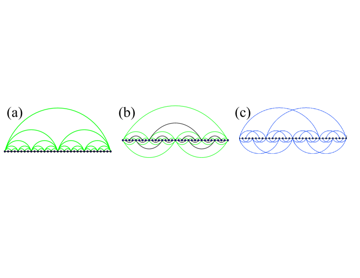
Figure 1: Depiction of hierarchical networks: (a) MK1, (b) HN5, and (c) HNNP. For all networks the recursive pattern that scales to the thermodynamic limit is evident. Each network features regular geometric structures, such as a one-dimensional backbone, and a distinct set of small-world links. While MK1 and HN5 are planar, HNNP is non-planar.

Such a non-linear approach towards the transition contrasts with the behavior of the equivalent exponent, defined via the susceptibility, on the same networks near the critical temperature for the Ising model [cite future work], and also with the predictions of the universal theory for these transitions (Boettcher and Brunson, arXiv:1209.3447), which would obtain a linear correction generically. In a companion Communication, we will illuminate the connection between Ising and percolation critical behavior on these networks using the $q$-state Potts model in its analytic continuation for non-integer values of $q$. There, we find that the quadratic corrections persist for all $q<2$, including percolation ($q\to 1$) merely as a special case. Only when $q\geq 2$, including the Ising model ($q=2$) as the $marginal$ case, do linear corrections dominate. In the future, we will extend our Potts-model analysis to entire families of complex networks.

This paper is organized as follows: In the following Sec. II, we introduce the networks used in our current study. Then, in Sec. III, we first review the RG-methods used to analyze the bond percolation transition for the case previously considered in Ref. (Boettcher et al., 2012) and then apply the same techniques in Sec. IV to the Hanoi networks; we extract the exact quadratic corrections for bond percolation in the cluster size exponent $\Psi$ for these networks while deferring many of the technical details of the calculation to the Appendix. In Sec. V we show that such non-linear corrections also characterize the site percolation transition. In Sec. VI, we finish with our conclusions and suggestions for future work.

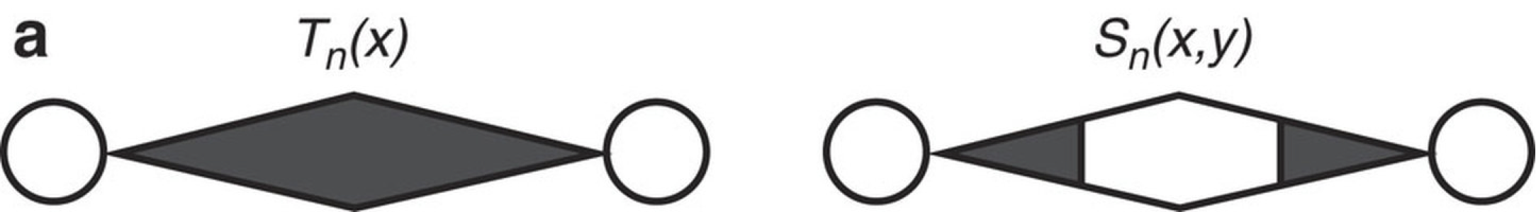
Figure 2: Diagrammatic definition of generating functions $T_{n}(x)$ and $S_{n}(x,y)$ in Eqs. (5) for MK1 in Fig. 1. End sites are represented by open circles and clusters by shaded areas. $T_{n}(x)$ consists of one spanning cluster, labeled $x$, which connects both end-sites and $S_{n}(x,y)$ consists of two non-spanning clusters, $x$ and $y$, each connected to one end-site. Isolated clusters not containing either of the end sites are ignored.

II Small-World Hyperbolic Networks

The models we are studying here are familiar hierarchical networks that have become popular because they provide exact results for complex processes by way of the real-space renormalization group. MK1, depicted in Fig. 1(a), is the one-dimensional version of the small-world Migdal-Kadanoff hierarchical diamond lattice (Hinczewski and Berker, 2006), which has been used previously to prove the existence of the discontinuous transition in ordinary percolation (Boettcher et al., 2012). MK1 is recursively generated starting with two sites connected by a single edge at generation $n=0$. Each new generation recursively combines two sub-networks of the previous generation and adds single edge connecting the end sites. As a result, the n^th generation contains $2^{n}+1$ vertices, $2^{n}$ backbone bonds, and $2^{n}-1$ small-world bonds.

To show that this discontinuity persists for more complicated but hierarchical structures, we consider here also the Hanoi networks HN5 and HNNP, also shown in Fig. 1(b-c). A similar recursive procedure as described above for MK1 is also applied to obtain each new generation, however, due to their more complicated structure their basic building block at $n=0$ consists of a triangle of three sites. For these Hanoi networks, the existence of a non-trivial bond-percolation transition has been demonstrated previously (Boettcher et al., 2009). HN5 is similar to MK1 but requires a coupled system of RG-recursions. It also can be easily adapted to complement previous investigations of site-percolation (Hasegawa and Nemoto, 2013) in a non-trivial fashion. HNNP is special in that it is a non-planar graph, and aspect that is missing from other hierarchical networks.

III Review of Cluster Renormalization in Bond Percolation

Before we apply it to calculate exact expressions for the scaling of the average cluster size for HN5 and HNNP in the next section, we first review briefly the formalism needed to analyze the average cluster size near the bond-percolation transition, as used for MK1 in Ref. (Boettcher et al., 2012). While a full understanding the dynamics of cluster formation near the discontinuous percolation transition requires knowledge of the entire cluster-size distribution, already the average size of the largest cluster $\left\langle s_{{\rm max}}\right\rangle_{n}$ at generation $n$ provides profound insights. In particular, we will be focused on the system-size scaling of $\left\langle s_{{\rm max}}\right\rangle_{n}$ for $p\to p_{c}$. In the following, we derive $\left\langle s_{{\rm max}}\right\rangle_{n}$ using cluster generating functions.

III.1 Cluster Generating Function for MK1:

We review briefly the procedure described in Ref. (Boettcher et al., 2012) for MK1. There, the generating functions were obtained by introducing merely two quantities: the probability $t_{i}^{(n)}(p)$ that both end-sites are connected to the same cluster of size $i$, and the probability $s_{i,j}^{(n)}(p)$ that the left end-site is connected to a cluster of size $i$ and the right end-site to a different cluster of size $j$. The generating functions, as depicted in Fig. 2, are defined as

$$T_{n}(x)= \sum_{i=0}^{\infty}t_{i}^{(n)}(p)\,x^{i}$$ (2)

$$S_{n}(x,y)= \sum_{i=0}^{\infty}\sum_{j=0}^{\infty}s_{i,j}^{(n)}(p)\,x^{i}\,y^{j}.$$ (3)

The recursion relations for these generating functions can be obtained by considering all possible configurations on three sites, as shown in Fig. 3, taking into account the cluster sizes as described in Ref. (Boettcher et al., 2012). The graphlets on three sites are assigned to the correct two-site graphlet in the next generation, and the weights of all the graphlets that contribute to the same higher-generation graphlet are added together to get the recursion relations,

$$T_{n+1}(x)=\, xT_{n}^{2}(x)$$

$$+p\left[2xT_{n}(x)S_{n}(x,x)+S_{n}(x,1)S_{n}(1,x)\right],$$ (4)

$$S_{n+1}(x,y)=\, (1-p)\left[xT_{n}(x)S_{n}(x,y)+yT_{n}(y)S_{n}(x,y)\right.$$

$$\left.\qquad+S_{n}(x,1)S_{n}(1,y)\right],$$ (5)

as indicated in Fig. 3 and discussed in more detail in Appendix VIII.1.1.

Figure 3: Diagrammatic evaluation of generating functions for MK1. All graphlets contributing to $T_{n+1}(x)$ and $S_{n+1}(x+y)$ in the nth generation. Graphlets (a-e) have end-to-end connections and contribute to $T_{n+1}(x)$ while (f-h) contribute to $S_{n+1}(x,y)$. The contribution of each graphlet is (a) $xpT_{n}^{2}(x)$ (b) $xpT_{n}(x)S_{n}(x,x)$ (c) $xpT_{n}(x)S_{n}(x,x)$ (d) $pS_{n}(x,1)S_{n}(1,x)$ (e) $x(1-p)T_{n}^{2}(x)$ (f) $x(1-p)T_{n}(x)S_{n}(x,y)$ (g) $y(1-p)T_{n}(y)S_{n}(x,y)$ (h) $(1-p)S_{n}(x,1)S_{n}(1,y)$. The recursion can be obtained by adding weights (a-e) for $T_{n+1}(x)$ and (f-h) for $S_{n+1}(x,y)$ resulting in Eq. (5). See Appendix VIII.1 for an algorithm to automate the evaluation.

III.2 Fixed Point Analysis for Average Cluster Size:

The recursion equations in Eq. (5) can be simplified by combination them into a vector $\vec{V}_{n}\left(x\right)=[T_{n}\left(x\right),S_{n}\left(x,x\right),S_{n}\left(x,1\right)]$ of distinct observables, where we focus on the largest cluster $x$ only. The RG can now be written as

$$\vec{V}_{n+1}(x)=\vec{F}\left(\vec{V_{n}}(x),x\right)$$ (6)

for the nonlinear vector-function $\vec{F}$ that derives from Eqs. 5. As Eq. (2) suggest, the average size of a spanning cluster (which dominate in the cluster-size distribution) is generated by $\left\langle s\right\rangle\sim T_{n}^{\prime}\left(x=1\right)$; any form of $S_{n}$ does not affect to the spanning cluster and its contributions prove subdominant. We obtain $T_{n}^{\prime}\left(x=1\right)$ in terms of $T_{n}=T_{n}\left(x=1\right)$ and $p$ by linearizing the recursion relation in Eq. 6

$$\frac{\partial\vec{V}_{n+1}}{\partial x}=\frac{\partial\vec{F}}{\partial\vec{V}}\left(\vec{V_{n}}\right)\cdot\frac{\partial\vec{V}_{n}}{\partial x}+\frac{\partial\vec{F}}{\partial x}\left(\vec{V_{n}}\right),$$ (7)

near $x=1$. Eq. (6) itself at $x=1$ (where $S_{n}=1-T_{n}$) reduces for MK1 in each component of $\vec{V}$ to

$$T_{n+1}=p+\left(1-p\right)T_{n}^{2}\qquad\left(T_{0}=p\right)$$ (8)

with fixed point $T_{\infty}=\lim_{n\to\infty}T_{n}$

$$T_{\infty}\left(p\right)=\left\{\begin{matrix}\frac{p}{(1-p)}&&0\leq p<\frac{1}{2}\\ 1&&\frac{1}{2}\leq p\leq 1,\end{matrix}\right.$$ (9)

providing the critical point $p_{c}=\frac{1}{2}$, where any spanning cluster also becomes extensive, see Fig. 4(a).

Ignoring the subdominant inhomogeneity in Eq. (7), the remaining homogeneous linear system gives the dominant contribution for $V_{\infty}^{\prime}$, i.e. $T_{\infty}^{\prime},S_{\infty}^{\prime}$. The largest eigenvalue $\lambda$ of the coefficient-matrix $\frac{\partial\vec{F}}{\partial\vec{V}}\left(\vec{V_{\infty}}\right)$ at the fixed point $T_{\infty}\left(p\right)$ becomes for MK1

$$\lambda=\left\{\begin{matrix}\frac{1+3p-4p^{2}}{2(1-p)}+\sqrt{\frac{1-p(1-4p)^{2}}{4(1-p)}}&&0\leq p<\frac{1}{2}\\ 2&&\frac{1}{2}\leq p\leq 1.\end{matrix}\right.$$ (10)

Finally, we obtain the order parameter $P_{\infty}$ as

$$P_{\infty}=\frac{\left\langle s_{{\rm max}}\right\rangle}{N}\sim\frac{T_{\infty}^{\prime}}{N}\sim N^{\Psi\left(p\right)-1}$$ (11)

with the fractal exponent(12)

$$\Psi\left(p\right)=\log_{2}\lambda.$$ (12)

Note that this implies that the largest cluster below the transition is already diverging with a non-zero power of the system size, although in a sub-extensive manner, $\Psi<1$ for $p<p_{c}$, such that $P_{\infty}\to 0$ for $N\to\infty$. These spanning, sub-extensive clusters exist, albeit with finite probability given by $T_{\infty}\left(p\right)$ in Eq. (9), for all $0<p<p_{c}$. This behavior for hyperbolic systems contrasts with that of regular lattices, where such sub-extensive clusters with fractal scaling only exist for $p=p_{c}$ and $\Psi(p)\equiv 0$ for $p<p_{c}$ such that all clusters remain finite or at most diverge logarithmically in $N$.

In Fig. 5(a), we show a plot of $P_{\infty}(p)$ for MK1 evaluated after $n=10^{k}$ iterations using Eq. (7) displayed for $k=1,...,5$ corresponding to system sizes up to $N\simeq 2^{n}\sim 10^{3010}$ sites. $P_{\infty}$ converges slowly to zero for $p<p_{c}=\frac{1}{2}$. At and above $p_{c}$, it can be shown using Eq. 7 that $T_{n}^{\prime}$ is monotonically increasing with $n$ while being bounded above by $1$, thus the order parameter is positive definite for $\frac{1}{2}\leq p<1$. The order parameter $P_{\infty}$ changes discontinuously from $0$ to $0.609793...$ at $p=p_{c}$ and converges to $1$ for $p\rightarrow 1$. A more detailed discussion, including a proof of the discontinuity, is provided in Ref. (Boettcher et al., 2012).

Figure 4: Phase diagram for the probability of a spanning cluster (a) $T_{\infty}$ for MK1 in Eq. (9), (b) $R_{\infty}$ for HN5 in Eq. (36), and (c) $R_{\infty}$ for HNNP in Eq. (35) (for $x=1$), all as a function of bond probability $p$. Black lines mark stable fixed points, and red-shaded lines are unstable fixed point solutions. The critical transition, at which the probability of any site to belong to the largest cluster becomes finite and that cluster becomes extensive, occurs exactly when the probability of a spanning cluster becomes unity, at $p_{c}=\frac{1}{2}$ for MK1 and $p_{c}=2-\phi=0.38197\ldots$ for both, HN5 and HNNP (Boettcher et al., 2009). However, in all cases, there is a non-zero probability for a spanning cluster, albeit sub-extensive, even below $p_{c}$, due to the hyperbolic nature of these hierarchical networks. For MK1 and HN5, such a cluster can exist for all $0<p<p_{c}$, while for HNNP it disappears below the branch-point singularity at $p_{l}=0.31945\ldots$. Note that in each case the transition occurs at the intersection of two lines of stable fixed points.

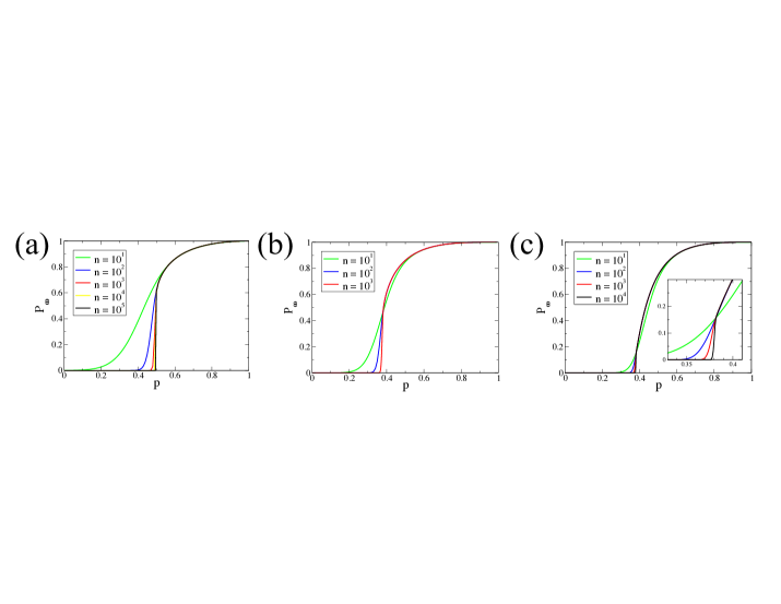
Figure 5: Discontinuity in the percolation order parameter $P_{\infty}(p)$ for (a) MK1, (b) HN5, and (c) HNNP, each for $n=10^{k}$ iterations for some integer $k$. In each case, $P_{\infty}$ converges slowly to zero just below $p_{c}$, and at $p_{c}$, $P_{\infty}$ changes discontinuously. The discontinuity decreases left to right, and is barely visible for HNNP, see inset.

III.3 Scaling Behavior near the Transition

From Eqs. (10-12) it is now easy to determine the scaling behavior for the average cluster size near the transition. By expanding the eigenvalue $\lambda$ in Eq. (10) for $p\to p_{c}$ from below, we find that the leading behavior only has quadratic corrections, and inserting into Eq. (12) results in

$$\Psi(p)\sim 1-\frac{8}{{\rm\ln 2}}\left(p-p_{c}\right)^{2},\qquad p\nearrow p_{c}=\frac{1}{2},$$ (13)

which rapidly approaches unity. This implies that the largest (spanning) cluster that dominates the distribution is nearly extensive already much before the discontinuous transition is reached. RG can only determine the probability $T_{\infty}$ and average size $\left\langle s_{{\rm max}}\right\rangle\sim T_{\infty}^{\prime}$ of the spanning cluster. Their sub-extensive nature for $p<p_{c}$ would allow in principle for a diverging number of such clusters. Our simulations show that already for small systems the largest cluster is almost certainly connected to at least one end-site near $p_{c}$. (In fact, for MK1 we could have just as well defined $\left\langle s_{{\rm max}}\right\rangle\sim T_{\infty}^{\prime}+{\cal S}_{\infty}^{\prime}$ to account not just for spanning but all end-site connected clusters, without affecting the scaling.) However, as we will see for HNNP, the non-extensive clusters further below $p_{c}$ may well be purely internal, with zero probability of spanning between any end-sites.

In light of the discussion regarding universal behavior in hyperbolic networks (Boettcher and Brunson, arXiv:1209.3447; Nogawa and Hasegawa, arXiv:1312.4697), it is interesting to also explore the scaling behavior of the order parameter on its approach to the discontinuity from above the transition. Numerically, with the RG, we find that a fit to

$$P_{\infty}\left(p\right)\sim P_{\infty}\left(p_{c}\right)+A\left(p-p_{c}\right)^{\beta}\qquad\left(p\searrow p_{c}\right)$$ (14)

is quite consistent with a simple, linear approach, i.e., $\beta=1$, see Fig. 6(a).

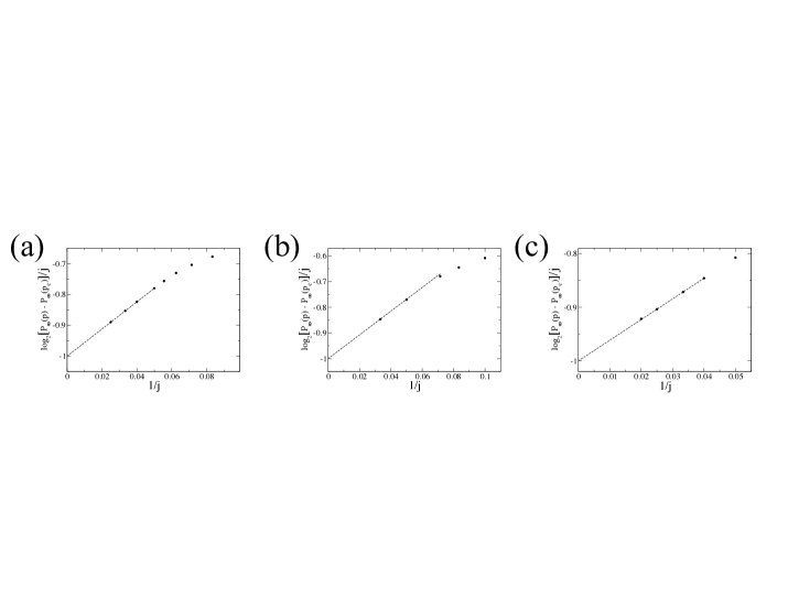
Figure 6: Scaling of the order parameter $P_{\infty}(p)$ for $p\searrow p_{c}$ according to Eq. (14) for (a) MK1, (b) HN5, and (c) HNNP. In each case, taking $p-p_{c}=\frac{1}{2^{j}}$, we plot $\log_{2}\left[P_{\infty}\left(p\right)-P_{\infty}\left(p_{c}\right)\right]/j$ vs. $1/j$ which linearly extrapolates to $\beta\sim 1$ as the intercept at $j\to\infty$, i.e., $p\to p_{c}$ .

IV Cluster-Size Scaling for Hanoi Networks

In the following, we will apply the formalism from Sec. III to the Hanoi networks HN5 and HNNP in Fig. 1(b-c). Their phase diagram, as shown in Fig. 4(b-c), has already been discussed in Ref. (Boettcher et al., 2009). To obtain their average cluster size requires the automated algorithm developed in the Appendix, due to the substantial combinatorial effort to enumerate their conformations. We will focus here on the more interesting case of HNNP first and then merely report equivalent results for HN5, without the details.

Despite of the added complexity, we find remarkably similar results near the transition for these networks, as compared to MK1, and only some distinctly interesting features for HNNP in the “patchy” regime below $p_{c}$. Such robust behavior suggests universal features (Boettcher and Brunson, arXiv:1209.3447; Nogawa and Hasegawa, arXiv:1312.4697), which can be traced back to the fundamental phase diagram shared by all three networks, as is evident from Fig. 4. For comparison, this bond-percolation behavior is not shared by another hierarchical network, MK2, which mutatis mutandis has quite a distinct phase diagram (Boettcher et al., 2009; Berker et al., 2009), leading instead to a BKT transition. See Ref. (Nogawa and Hasegawa, arXiv:1312.4697) for an interpolation between both cases.

In the Appendix, Sec. VIII.1.2, we show how to obtain the RG-recursions for the cluster generating functions. While otherwise similar to the discussion in Sec. III.1, HNNP (as well as HN5) requires four such functions to account for all possibilities, of having clusters linking any combination of three end-sites or remain isolated, even after accounting for all symmetries of the network. The resulting recursions, Eqs. (35), are similar to those for MK1 in Eqs. (5), although rather more involved. In the end, we only care for the dominant cluster, which we label $x$, and consider each possible contribution from one RG-step to the next while disregarding sub-dominant clusters by setting $y=z=1$. Note that even clusters that are disconnected from any end-site at one step could significantly contribute at the next via the small-world bonds that are linking graphlets between consecutive RG-steps. In the end, we can identify ten distinct observables that form a closed set of recursions. When combined into a single vector,

$$\vec{V}_{n}(x) = \left[R_{n}(x),S_{n}(x,x),S_{n}(x,1),U_{n}(x,x),\right.$$

$$\quad U_{n}(x,1),N_{n}(x,x,x),N_{n}(x,x,1),$$

$$\left.\,N_{n}(x,1,x),N_{n}(x,1,1),N_{n}(1,x,1)\right],$$

these satisfy the equivalent recursion in (6), with the nonlinear RG-flow given by Eqs. (35).

To zeroth order, at $x=1$, Eq. (6) gives the recursion relation for percolation of the HNNP graph as derived in Ref. (Boettcher et al., 2009). The coupled recursion relations in ($R_{n},S_{n},U_{n},N_{n}$) result in the roots of a sextic polynomial, which can be solved numerically to get the probability of, say, the spanning cluster $R_{\infty}$ between the end-sites. Fig. 4(c) gives the phase diagram for HNNP representing the solutions of the sextic equation, which correspond to the probability $R_{\infty}$ for $0<p<1$. HNNP provides a unique example of a network in which the probability of the dominant cluster to touch any end-site vanish below some finite value $0<p_{l}<p_{c}$. In Ref. (Boettcher et al., 2009) this was interpreted as a second, lower, critical point, where below $p_{l}$ neither a spanning nor an extensive cluster exists while between $p_{l}$ and $p_{c}$ at least a spanning cluster exists that does not need to be extensive, due to the hyperbolic structure of the network. That spanning cluster becomes extensive only above $p_{c}$, the true critical percolation point with non-zero order parameter, $P_{\infty}>0$. However, as was shown in Ref. (Hasegawa and Nogawa, 2013), even below the non-zero $p_{l}$ in HNNP a diverging cluster remains and $\Psi(p)$ defined in Eq. (1) remains positive for all $p>0$. At $p_{l}$, $\Psi(p)$ merely jumps discontinuously to a lower but finite value, yet, diverging clusters that connect end-sites are almost certainly absent. Any diverging cluster is fully contained inside HNNP.

The nature of the largest cluster can be studied by looking at the first-order term in the Taylor expansion, Eq. 7, of the vector $\vec{V}_{n}(x)$ in Eq. IV. For HNNP the Jacobian $\frac{\partial\vec{F}}{\partial\vec{V}}\left(\vec{V}_{n}\right)$ at $x=1$ consists now of a $10\times 10$ matrix and the inhomogeneity is a $10\times 1$ matrix. For large system sizes ($n\to\infty$) at $x=1$, it can be shown that the inhomogeneity is subdominant, leaving a homogeneous equations. As before, the largest eigenvalue of the Jacobian gives the scaling exponent $\Psi(p)$ for the largest cluster in the network from Eq. (12), as shown in Fig. 7. It shows that $\Psi(p)<1$ for $p_{l}<p<p_{c}$, but $\Psi(p)$ drops to zero discontinuously at $p_{l}$ and vanishes for $p<p_{l}=0.31945\ldots$, since the cluster measured by the RG is conditioned on being rooted at an end-site. The RG misses diverging clusters that that do not span the network which apparently dominate below $p_{l}$ (Nogawa and Hasegawa, arXiv:1312.4697). In any case, since $\Psi(p)<1$, Eq. (11) ensures that $P_{\infty}\equiv 0$ for all $0\leq p<p_{c}$.

Figure 7: Plot of the fractal exponent $\Psi(p)$ for HNNP. The behavior of $\Psi(p)$ for $p_{l}<p<p_{c}=0.38197\ldots$ (full line) is obtained by exact evaluation of the Jacobian matrix, which develops a branch-point singularity at $p_{l}=0.31945\ldots$. Ref. (Hasegawa and Nogawa, 2013) has provided a lower bound, $\Psi(p)=\log_{2}\left(1+\sqrt{1+8p}\right)-1$ for $p<p_{l}$ (dashed line), suggesting a discontinuity in the scaling of the largest cluster at $p_{l}$ (dotted line) when spanning clusters emerge.

Near $p_{c}=2-\phi$, where $\phi=\left(\sqrt{5}+1\right)/2$ is the “golden section”, we again find a percolation transition with a discontinuous jump in the order parameter $P_{\infty}$. By evolving the recursion equations (7) for $V_{n}^{\prime}$ , the order parameter can be rigorously shown to have monotone convergence to non-zero values at and above $p_{c}$, see Fig. 5(c). For $p\nearrow p_{c}$ , the way $\Psi(p)$ approaches unity can be found through considering the secular equation

$$0=\det\left\{V_{\infty}^{\prime}-\left(2-a_{1}\epsilon+a_{2}\epsilon^{2}+\ldots\right)\times\mathbf{I}\right\},$$ (16)

expanded in terms of $\epsilon=p_{c}-p\ll 1$, where $\mathbf{I}$ is the identity matrix. Note that at $p_{c}$, the largest eigenvalue of $V_{\infty}^{\prime}$ is $\lambda=2$, around which we expand. Since the percolation probabilities at $p_{c}$ are given by $R_{\infty}=1,S_{\infty}=U_{\infty}=N_{\infty}=0$, we assume an expansion of the percolation probabilities as $R_{\infty}=1-\rho_{1}\epsilon+\rho_{2}\epsilon^{2}$, $S_{\infty}=\sigma_{1}\epsilon+\sigma_{2}\epsilon^{2}$, $U_{\infty}=\nu_{1}\epsilon+\nu_{2}\epsilon^{2}$, and $N_{\infty}=\eta_{1}\epsilon+\eta_{2}\epsilon^{2}$. To satisfy Eq. (16), each coefficient in powers of $\epsilon$ should be zero. As a result, we find that linear corrections to the eigenvalue $\lambda$ vanish, i.e., $a_{1}=0$. Using conservation of probability, $\rho_{i}+\sigma_{i}+\upsilon_{i}+\eta_{i}=0$, for each $i\geq 1$ at $p=p_{c}$, we find a non-vanishing quadratic correction, $a_{2}=a_{2}(\rho_{1},\sigma_{1},\nu_{1},\eta_{1})=-\frac{5}{16}\left(38+17\sqrt{5}\right)$, for which the second-order corrections in the percolation probabilities proved irrelevant. Hence, Eq. (12) yields

$$\Psi_{{\rm HNNP}}(p)\sim 1-\frac{5\left(38+17\sqrt{5}\right)}{32\log_{e}(2)}\left(p_{c}-p\right)^{2}+\ldots, \quad p\nearrow p_{c}.$$ (17)

For HN5, by using the same cluster generating functions as for HNNP in the Appendix, we obtain their RG recursions in (36). Again, the resulting equations for the cluster size are too complicated to express or solve in closed form. But it is easy to evaluate their phase diagram in Fig. (4)(b) for $R_{\infty}$, as well as the order parameter $P_{\infty}$ in Fig. (5)(b) to any desired accuracy. Here, the same local analysis near $p_{c}$ as for HNNP yields for HN5:

$$\Psi_{{\rm HN5}}(p)\sim 1-\frac{5\left(677+304\sqrt{5}\right)}{484\log_{e}(2)}\left(p_{c}-p\right)^{2}+\ldots, \quad p\nearrow p_{c}.$$ (18)

As for MK1 and HNNP, almost extensive clusters in HN5 emerge well before the transition, with $\Psi(p)$ varying quadratically. It suggests that the quadratic dependence below $p_{c}$ might be universal for hierarchical networks with discontinuous percolation transitions. Above $p_{c}$, the scaling of $P_{\infty}$ in Eq. (14) for both, HN5 and HNNP, also provides $\beta\sim 1$, as shown in Fig. 6(b-c).

V Cluster Size for Site Percolation

We supplement these findings with a unique result of even higher-order behavior in the site-percolation transition of HN5 in Fig. 1. The fragility of complex networks under random site-removal has recently been studied on hierarchical networks (Hasegawa and Nemoto, 2013). It was shown that there is no threshold at which the network preserves an extensive cluster, i.e., $p_{c}=1$, yet, similar quadratic corrections in scaling to the formation of an extensive cluster for $p\to 1$ are also found there. Hence, we would expect that cluster formation near this discontinuity is generic for both, bond- and site-percolation. In light of this, the cubic corrections we report here for HN5 may provide an alternative, special case and a new clue in understanding cluster formation.

With the framework for studying bond percolation on hierarchical networks established in Sec. III, we apply the same protocols to study site percolation. HN5 can be assembled recursively by combining all possible triangle permutations listed in Fig. 8 through mergers as explained in Fig. 9. Clusters are labeled $x$ if they at least touch the left-most root site, $y$ if they do not touch the left root but at least the right-most root site, and $z$ if they only reach the central root site. If all root sites are unoccupied, there are no countable clusters to label, and the argument becomes unity. Extra small-world bonds, as in the construction of HN5 in Fig. 9, may combine clusters, which entails a relabeling dictated by the same priority.

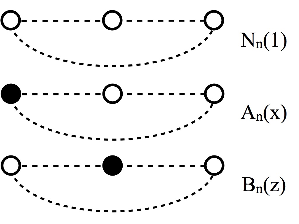
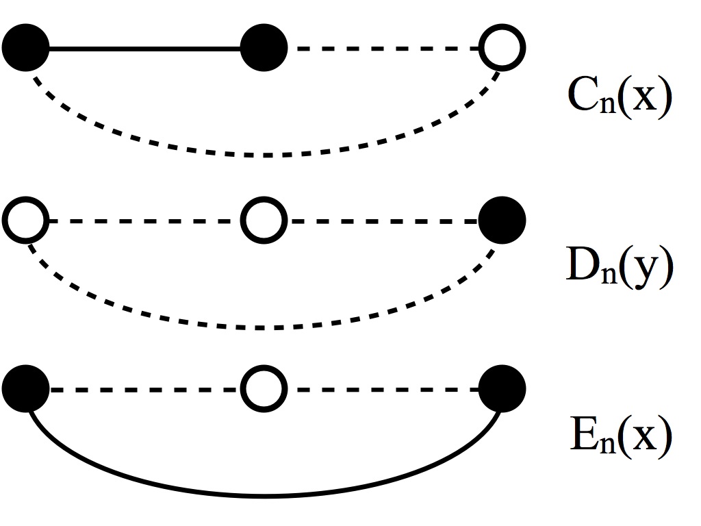
Figure 8: Depiction of elementary HN5 graphlets for site percolation. Listed are all ($2^{3}=8$) three-site graphlets used in the recursive composition of Hanoi networks. Filled (or unfilled) circles mark occupied (or unoccupied) sites, each with independent probability $p$ (or $1-p$). The arguments $x$, $y$, and $z$ indicate that each triangle harbors a single cluster, represented by a polynomial generating function in that variable. A full line corresponds to an existing connection between occupied sites, and a dashed line is a possible, but unrealized, connection when one adjacent site is unoccupied. Note that $A_{n}$ and $D_{n}$, and $C_{n}$ and $F_{n}$ are simply mirror images of each other that satisfy the same recursions; hence, we can eliminate $D_{n}$ and $F_{n}$ from the recursions in the end.

Figure 9: Demonstration of the merging of elementary graphlets into a graphlet of the next generation in HN5, the generic five-site structure being exhibited by the lower diagram. Here, graphlets for $C_{n}\left(x\right)$ and $B_{n}\left(y\right)$ (defined in Fig. 8) are merged by overlapping at the highlighted inner sites that become one. Adding the new long-range bonds, a graphlet of HN5 is formed (below). The lower one of those bonds unifies the occupied sites left and right into a single cluster, reducing the labeling from $x$ and $z$ into a single label $x$. Renormalization now consists of eliminating the 2nd and 4th site and attributing their properties to the respective root-sites (left, right and center sites). Here, for instance, there is merely one cluster labeled $x$ that only connects to the left root, the center and right root remain empty. Thus, this graphlet renormalizes into the type $A_{n+1}\left(x\right)$, also defined in Fig. 8. The entire RG consists of evaluating such a merger for all $2^{5}=32$ possible site-occupancies in the HN5 graphlet to obtain the recursions in Eq. (19). Of course, mergers can only be realized when the overlapping inner sites are in the same state; that merger has to be corrected for by dividing out $1/\left(1-p\right)$ when an empty site is over-counted, as in this example, or by $1/\left(xp\right)$ when an overlapping occupied site is over-counted. Incidentally, this case (and its mirror image) is the only graphlets among all 32 for which the lower long-range bond – the distinguishing feature between MK1 and HN5 – makes a difference; otherwise the site from $B_{n}\left(y\right)$ on the right would be disconnected from any root and would remain uncounted.

Based on these rules explained in Fig. 9, applied to the merger of all possible graphlets in Fig. 8, the following RG-recursions for the cluster generating functions are derived:

$$N_{n+1}\left(1\right) = \frac{1}{1-p}\left[N_{n}\left(1\right)+B_{n}\left(1\right)\right]^{2},$$ (19)

$$A_{n+1}\left(x\right) = \frac{1}{1-p}\left\{\right.\left[A_{n}\left(x\right)+C_{n}\left(x\right)\right]\left[N_{n}\left(1\right)+B_{n}\left(1\right)\right]$$

$$+C_{n}\left(x\right)\left[B_{n}\left(x\right)-B_{n}\left(1\right)\right]\left.\right\},$$

$$B_{n+1}\left(z\right) = \frac{1}{xp}\left[A_{n}\left(z\right)+C_{n}\left(z\right)\right]^{2},$$

$$C_{n+1}\left(x\right) = \frac{1}{xp}\left[A_{n}\left(x\right)+C_{n}\left(x\right)\right]\left[E_{n}\left(x\right)+G_{n}\left(x\right)\right],$$

$$E_{n+1}\left(x\right) = \frac{1}{1-p}\left[A_{n}\left(x\right)+C_{n}\left(x\right)\right]^{2},$$

$$G_{n+1}\left(x\right) = \frac{1}{xp}\left[E_{n}\left(x\right)+G_{n}\left(x\right)\right]^{2}.$$

Here, we already have exploited a mirror symmetry between $A_{n}$ and $D_{n}$ and between $C_{n}$ and $F_{n}$ to simplify the equations. The initial conditions for these RG-recursions are:

$$N_{0}\left(x\right)=\left(1-p\right)^{3},~{}~{}~{}~{}\qquad A_{0}\left(x\right)=xp\left(1-p\right)^{2},$$

$$B_{0}\left(z\right)=zp\left(1-p\right)^{2},~{}\qquad C_{0}\left(x\right)=x^{2}p^{2}\left(1-p\right),$$

$$E_{0}\left(x\right)=x^{2}p^{2}\left(1-p\right),\qquad G_{0}\left(x\right)=x^{3}p^{3}.$$ (20)

Unlike the recursions for the bond-cluster generating functions, for example, Eq. (9) for MK1, here the site-cluster generating functions themselves do not satisfy interesting recursions at $x=1$. For instance, $A_{n}\left(1\right)=A_{0}\left(1\right)=p\left(1-p\right)$ for all $n$ merely reflects the defining feature of the site-percolation cluster $A_{n}\left(x\right)$ of being occupying the left end-site but not the right end-site.

Note that without the seemingly minor distinction between $B_{n}\left(x\right)$ and $B_{n}\left(1\right)$ in the $A_{n+1}$-relation, as explained in Fig. 9, we could drastically reduce the recursions further by defining

$$T_{n}\left(x\right) = \frac{1}{x^{2}p^{2}}\left[E_{n}\left(x\right)+G_{n}\left(x\right)\right],$$ (21)

$$S_{n}\left(x\right) = \frac{1}{xp\left(1-p\right)}\left[A_{n}\left(x\right)+C_{n}\left(x\right)\right],$$

which converts Eqs. (19) into those for MK1 in Ref. (Hasegawa and Nemoto, 2013). Instead, we have to evolve the entire set of five $x$-dependent relations for the RG-flow in Eqs. (19).

Figure 10: Plot of $\Psi=\log_{2}\lambda$ in HN5 as a function of the site-occupation probability $p$, obtained from largest solution of the eigenvalue Eq. (24). Noticeable is the slow rise for $p\to 1^{-}$ derived in Eq. (25).

Defining

$$\vec{V}_{n}(x) = \left[A_{n}(x),B_{n}(x),C_{n}(x),E_{n}(x),G_{n}(x)\right]$$ (22)

and following the discussion in Sec. III, we obtain from Eqs. (19) at $x=1$:

$$\frac{\partial\vec{F}}{\partial\vec{V}}\left(\vec{V}_{\infty}\right)=\left(\begin{array}[]{ccccc}1-p&p^{2}&1-p&0&0\\ 2\left(1-p\right)&0&2\left(1-p\right)&0&0\\ p&0&p&1-p&1-p\\ 2p&0&2p&0&0\\ 0&2\left(1-p\right)&0&0&0\end{array}\right).$$ (23)

where we used the IC in Eqs. (20) and the fact explained above that $\vec{V}_{n}\left(1\right)=\vec{V}_{0}\left(1\right)$ for any $n$ for site-percolation generating functions. Then, the largest eigenvalue is the largest root of the cubic equation

$$0=4p^{3}-4p^{4}+2p^{3}\lambda-(1+2p)\lambda^{2}+\lambda^{3}.$$ (24)

Again, as in Eq. (12), it is $\Psi\left(p\right)=\log_{2}\lambda$, which is shown in Fig. 10. It is remarkable that, although $\Psi\left(p\right)$ varies smoothly between 0 and 1, near $p=1$ we find only a cubic correction near $p_{c}=1$:

$$\Psi\left(p\right)\sim 1-\frac{2}{\ln 2}\left(1-p\right)^{3},\qquad p\nearrow p_{c}=1.$$ (25)

VI Conclusions

Our investigation of properties of the cluster formation near the discontinuous percolation transition in hyperbolic networks affirms the robustness of the observed finite-size scaling of the largest cluster in the system. Our study considers more complicated classes of networks than before, and extends the analysis to include both, bond- and site-percolation. To obtain our results, we present an automated means of graph counting, which are essential to accomplish the RG-recursions for entire functions that are the generators for the cluster sizes. In the Appendix, we present these methods in somewhat more detail so that they can serve as a blueprint for similar efforts in the future.

Our RG study can merely implicate interesting scaling features in the evolution of the emergent cluster; only detailed simulation can provide sufficient insight into the mechanics of their formation. In a parallel effort, we are currently studying bond percolation on these hyperbolic networks as the familiar limit $q\to 1$ of the $q$-state Potts model (SinghPotts). In this form, we also hope to better understand the connection between discontinuous percolation transitions and the phenomenology of critical transitions as found, for instance, in ferromagnets on these networks (Boettcher and Brunson, arXiv:1209.3447), which should be revealed by the interpolation between $1\leq q\leq 2$ in the analytic continuation of the Potts model.

VII Acknowledgments

We like to thank Trent Brunson, Tomoaki Nogawa, and Takehisa Hasegawa for fruitful discussions. This work was supported by Grants No. DMR-1207431 and No. IOS-1208126 from the NSF, and by Grant No. 220020321 from McDonnel Foundation.

VIII Appendix

VIII.1 Automated Graph Counting

The recursion relations (5) for MK1 are obtained by a process of graph counting depicted in Fig. (3). As the number of possible graphlets increases exponentially for more complicated hierarchical networks (e.g. HN5 and HNNP), automating the graph enumeration process $insilico$ makes it easier to obtain their recursion equations. Key to this process is the adjacency matrix ${\rm{A_{ij}}}$, which gives the information about the presence of single bonds between two sites in a graph.

VIII.1.1 Counting MK1 graphlets:

In the MK1-graphlet in Fig. 3a,

$$A_{a}=\begin{bmatrix}0&1&1\\ 1&0&1\\ 1&1&0\end{bmatrix}$$ (26)

is an example of an adjacency matrix when all possible bonds are present. The bonds are bi-directional, which results in a symmetric matrix, and the diagonal elements are zero, since there are no bonds that loop back to a site. In the case where two ends are not connected by a single bond, the adjacency matrix effectively searches for alternate paths to connect the two end-sites. In Fig 3e, for example, the small-world bond is missing, and sites 1 and 3 are not connected via a single bond. The adjacency matrix is thus,

$$A_{e}=\begin{bmatrix}0&1&0\\ 1&0&1\\ 0&1&0\end{bmatrix}.$$ (27)

By itself, the adjacency matrix gives the number of one-step end-site connections. To find the number of two-step end-site connections for a graphlet, the adjacency matrix must be squared. The off-diagonal elements of ${\rm{A}^{2}}$ give the number of possible paths between two sites that are exactly two hops long. Squaring the adjacency matrix in Fig. 3a (Eq. 26) gives

$$A_{e}^{2}=\begin{bmatrix}1&0&1\\ 0&2&0\\ 1&0&1\end{bmatrix}.$$ (28)

Since matrix element $A_{e,13}^{2}=1$, there exists only one possible path in which two-steps can be made to connect the end-sites. Since the maximum path length for the simple case of MK1 is two, only ${{A_{e,13}}}$ (one step) and ${A_{e,13}^{2}}$ (two steps) need to be checked for finding end-to-end connections.

The graphlets are classified as contributing to $T_{n+1}(x)$ or $S_{n+1}(x,y)$ depending on whether an end-to-end connection exists. The weights of the graphlets are calculated by first labeling the end-sites as $x$ and $y$. Both end-sites are labeled $x$ in fully-connected graphs contributing to $T_{n+1}(x)$, and unconnected graphs contributing to $S_{n+1}(x,y)$ contain the left end-site labeled $x$ and the right end-site labeled $y$.

For each graphlet in the $n^{th}$ generation, $x$ or $y$ is assigned to each site and $T_{n}(x)$ or $S_{n}(x,y)$ to each bond, depending on whether the end sites are attached. Isolated sites/clusters are assigned a weight of 1. The contribution of each graphlet in the $(n+1)^{th}$ generation is set as the product of the value assigned to the bonds and intermediate sites. For example, the two shaded backbone bonds of Fig. 3a indicate that the graphlet has two bonds of type $T_{n}(x)$. The small-world bond exists with probability $p$, and all the sites are connected to the same cluster. Therefore, the graphlet contributes to $T_{n+1}(x)$ in the next generation with weight $p\,x\,T_{n}^{2}(x)$. Similarly, for the graphlet in Fig. 3f, the backbone bonds are of the types $T_{n}(x)$ and $S_{n}(x,y)$. The small-world bond is absent with probability $1-p$, and the end-sites are connected to separate clusters, $x$ and $y$. Hence, this graphlet contributes to $S_{n+1}(x,y)$ in the next generation with weight $(1-p)\,x\,T_{n}(x)S_{n}(x,y)$.

Figure 11: Diagrammatic definition of generating functions for HNNP and HN5. Sites a, b and c represent the end-sites of the network. $R_{n}(x)$ consist of one cluster spanning all three end-sites, $S_{n}(x,y)$, $T_{n}(x,y)$ and $U_{n}(x,y)$ two clusters, one of which spanning two end-sites, and $N_{n}(x,y,z)$ represents non-spanning clusters which connect to at most one end-site.

VIII.1.2 Cluster Generating Function for HNNP:

The generating functions for the Hanoi network HNNP in Fig. 1 can be calculated using the same principles described for MK1. As in Sec. III.1, we define the generating functions for HNNP depicted in Fig. 11:

$$R_{n}(x) =\;\sum_{k=0}^{\infty}r_{k}^{(n)}(p)x^{k},$$ (29)

$$S_{n}(x,y) =\;\sum_{k=0}^{\infty}\sum_{l=0}^{\infty}s_{k,l}^{(n)}(p)x^{k}y^{l},$$ (30)

$$U_{n}(x,y) =\;\sum_{k=0}^{\infty}\sum_{l=0}^{\infty}u_{k,l}^{(n)}(p)x^{k}y^{l},$$ (31)

$$N_{n}(x,y,z) =\;\sum_{k=0}^{\infty}n_{k,l,m}^{(n)}(p)x^{k}y^{l}z^{m},$$ (32)

where we introduce the probabilities

• $r_{k}^{n}(p)$ that sites $a$, $b$ and $c$ are all connected within the same cluster of size $k$;

• $s_{k,l}^{n}(p)$ that $a$ and $b$ are mutually connected within a cluster of size $k$, and $c$ is connected to a separate cluster of size $l$;

• $t_{k,l}^{n}(p)$ that $a$ is connected to a separate cluster of size $k$, and $b$ and $c$ are mutually connected within cluster of size $l$;

• $u_{k,l}^{n}(p)$ that $a$ and $c$ are mutually connected within a cluster of size $k$, and $b$ is connected to a separate cluster of size $l$;

• $n_{k,l,m}^{n}(p)$ that $a$ is connected to a cluster of size $k$, $b$ is connected to a cluster of size $l$, and $c$ is connected to a cluster of size $m$, but all mutually disconnected.

The symmetry of $s_{k,l}^{n}$ and $t_{k,l}^{n}$ are included in the definition of $S_{n}(x,y)$ (Boettcher et al., 2009). As for MK1, the three end-notes themselves are not counted in the cluster size.

Figure 12: Example graphlet for HNNP. By looking at the elements of $A_{13}^{2}\;\&\;A_{13}^{2}$ of $A^{2}$, one can see that all the three end-sites are connected. So this graph contributes to $R_{n+1}(x)$ in the next generation. In fact all the sites are connected to the same cluster in this case, which can be verified by looking other element of $A,A^{2},A^{3}$ & $A^{4}$. Since all sites are connected to the same cluster (say of size $x$) and there is only one long range small world bond is present, the weight of the graphlet is $p(1-p)x^{2}R_{n}(x)S_{n}(x,x)/4.$

We want to obtain the system of RG recursions for generating functions, where $(R_{n+1},S_{n+1},U_{n+1},N_{n+1})$ are functions of $(R_{n},S_{n},U_{n},N_{n};p)$. The algorithm first generates the adjacency matrices corresponding to all possible ($2^{8}=256$) graphlets for the HNNP network. For each one of these graphlets the possibility of their contribution to one of $(R_{n+1},S_{n+1},U_{n+1},N_{n+1})$ in the next generation is checked using the adjacency matrices.

As an example of our graph counting algorithm for HNNP, we consider the graphlet in Fig. 12. At first glance it appears that there are two separate clusters of sizes $k$ and $l$. The adjacency matrix for this graphlet is

$$A\ =\ \begin{matrix}{\rm{Node}}&\begin{matrix}a&b&c&b^{\prime}&a^{\prime}\end{matrix}\\ \begin{matrix}a\\ b\\ c\\ b^{\prime}\\ a^{\prime}\end{matrix}&\begin{bmatrix}0&1&0&0&0\\ 1&0&1&0&1\\ 0&1&0&1&0\\ 0&0&1&0&0\\ 0&1&0&0&0\end{bmatrix}\end{matrix}$$ (33)

where the disconnect between sites $a^{\prime}$ and $b^{\prime}$ is indicated by $A_{4,5}=A_{5,4}=0$. After the sites $b$ and $b^{\prime}$ in Fig. 12 are decimated in the RG step, the remainder is matched with one of the graphlets in the generating function diagram in Fig. 11. Thus, only the matrix elements in Eq. 33 that connect end sites $a$ to $c$, $a$ to $a^{\prime}$, and $c$ to $a^{\prime}$ contribute to the recursion equations for the generating functions. In general, the matrix elements for $A^{4}$ must be checked for a five-point HNNP graphlet, since the maximum number of steps required to connect all end-sites is four. In our example,

$$A^{4}= \begin{bmatrix}3&0&4&0&3\\ 0&10&0&4&0\\ 4&0&6&0&4\\ 0&4&0&2&0\\ 3&0&4&0&3\end{bmatrix}.$$ (34)

Elements $A_{13}^{4}$, $A_{15}^{4}$, and $A_{53}^{4}$ are non-zero, indicating that the end sites ($a$, $c$, and $a^{\prime}$) form a contiguous cluster, where $a^{\prime}$ becomes connected by way of the small-world bond. The graphlet therefore renormalizes into an $R$-type bond. To determine its weight, we note that the sites $a$, $b$, and $c$ are connected via an $R_{n}$-type bond and the sites $c$, $b^{\prime}$, and $a^{\prime}$ form an $S_{n}$-type bond. Only the right-hand one of the small-world bonds is present. Hence, the total weight of this graphlet in the next generation is $p(1-p)\;x^{2}\;R_{n}(x)S_{n}(x,x)/4$. Here, $S_{n}$ becomes a function of $x$ in both arguments, since the small-world bond merges the previously disconnected clusters $x$ and $y$. The factor $1/4$ is due to the symmetry explained in Ref. (Boettcher et al., 2009).

This process is repeated for all 256 graphlets with our automated counting algorithm, where each graphlet is attributed to its appropriate next-generation graphlet. After adding the weights, the generating function recursion relations are found to be:

$$R^{\prime}(x) = \left\{xR\left(x\right)+pxU\left(x,x\right)+\left(1-p\right)U\left(x,1\right)\right\}^{2}+2pxR\left(x\right)\left\{pxN\left(x,x,x\right)+\left(1-p\right)N\left(x,1,x\right)\right\}$$ (35)

$$+pxS\left(x,x\right)\left\{\left(1-p\right)\left[xR\left(x\right)+U\left(x,1\right)\right]+2xR\left(x\right)+pxU\left(x,x\right)\right\}+\frac{3}{4}p^{2}x^{2}S\left(x,x\right)^{2},$$

$$S^{\prime}(x,y) = \frac{1-p}{2}S\left(x,y\right)\left\{px^{2}S\left(x,x\right)+py^{2}S\left(y,y\right)+x^{2}R\left(x\right)+y^{2}R\left(y\right)+\left(1-p\right)xy\left[R\left(x\right)+R\left(y\right)\right]\right.$$

$$\left.+\left[x+\left(1-p\right)y\right]U\left(x,1\right)+\left[y+\left(1-p\right)x\right]U\left(y,1\right)+p\left[x+y\right]^{2}U\left(x,y\right)+pxN\left(x,1,x\right)+pyN\left(y,1,y\right)\right\}$$

$$+\frac{p^{2}}{2}xyS\left(x,y\right)\left\{2U\left(x,y\right)+N\left(x,y,x\right)+N\left(y,x,y\right)\right\}+\left(1-p\right)N\left(x,1,y\right)\left\{p\left[x+y\right]U\left(x,y\right)\right.$$

$$\left.+\left(1-p\right)\left[xR\left(x\right)+yR\left(y\right)+U\left(x,1\right)+U\left(y,1\right)\right]\right\}+pxN\left(x,x,y\right)\left\{\left(1-p\right)\left[xR\left(x\right)+U\left(x,1\right)\right]+pyU\left(x,y\right)\right\}$$

$$+pyN\left(x,y,y\right)\left\{\left(1-p\right)\left[yR\left(y\right)+U\left(y,1\right)\right]+pxU\left(x,y\right)\right\},$$

$$U^{\prime}(x,y) = \frac{1}{4}px\left[\left(2-p\right)x+2\left(1-p\right)y\right]S(x,y)^{2}+pxS(x,y)^{2}\left\{\left(1-p\right)N\left(x,1,y\right)+pxN\left(x,x,y\right)\right\},$$

$$N^{\prime}\left(x,y,z\right) = \frac{1}{4}\left(1-p\right)^{2}\left[x+y\right]\left[y+z\right]S\left(x,y\right)S\left(y,z\right)+\frac{1-p}{2}\left[x+y\right]S\left(x,y\right)\left\{\left(1-p\right)N\left(x,1,z\right)+pxN\left(y,x,z\right)\right\}$$

$$+\left\{\left(1-p\right)N\left(x,1,y\right)+pzN\left(x,z,y\right)\right\}\left\{\left(1-p\right)N\left(x,1,z\right)+pxN\left(y,x,z\right)\right\}$$

$$+\frac{1-p}{2}\left[y+z\right]S\left(y,z\right)\left\{\left(1-p\right)N\left(x,1,y\right)+pzN\left(x,z,y\right)\right\}$$

Note that for $x=y=z=1$, i.e., when graphlets are counted irrespective of cluster sizes, these equations revert back to those previously listed in Ref. (Boettcher et al., 2009).

VIII.1.3 Cluster Generating Function for HN5:

The discussion on how to obtain the RG recursion equations for the cluster generating functions of HN5 parallels that for HNNP above. The definition of the generating functions in Eqs. 29, as illustrated in Fig. 11, equally apply to HN5. The main difference originates with the structure of small-world bonds, which leads to a planar graph for HN5 and a non-planar graph for HNNP. Then, our graph counting algorithm results in the following RG recursions:

$$R^{\prime}(x) = \left\{U(x,1)+xR(x)\right\}^{2}+\frac{1}{2}p^{2}x^{2}S(x,x)^{2}+2p\left\{N(x,1,x)U(x,1)+xS(x,x)\left[(1-p)U(x,1)+pxU(x,x)\right]\right\}$$ (36)

$$+pxR(x)\left\{2(1-p)N(x,1,x)+2pxN(x,x,x)+(3-p)xS(x,x)-2U(x,1)+2xU(x,x)\right\}$$

$$S^{\prime}(x,y) = (1-p)N(x,1,y)\left\{U(x,1)+U(y,1)+(1-p)\left[xR(x)+yR(y)\right]\right\}$$

$$+p(1-p)\left\{x^{2}R(x)N(x,x,y)+y^{2}R(y)N(x,y,y)\right\}+\frac{1-p}{4}S(x,y)\left\{px^{2}S(x,x)+py^{2}S(y,y)\right\}$$

$$+\frac{p(1-p)}{2}\left\{x^{2}\left[U(x,y)+U(x,x)\right]+y^{2}\left[U(x,y)+U(y,y)\right]\right\}+\frac{(1-p)^{2}}{2}\left[x+y\right]\left\{U(x,1)+U(y,1)\right\}$$

$$+\frac{1-p}{2}\left\{xR(x)\left[-py+x+y\right]+yR(y)\left[-px+x+y\right]\right\}$$

$$U^{\prime}(x,y) = p\left\{N(x,1,y)+\frac{1}{2}(1-p)\left[x+y\right]S(x,y)\right\}^{2}+p^{2}S(x,y)\left\{x^{2}N(x,x,y)+y^{2}N(x,y,y)\right\}$$

$$+\frac{p}{4}S(x,y)^{2}\left\{\left(1+p-p^{2}\right)x^{2}+2p(1-p)xy+(2-p)py^{2}\right\}$$

$$N^{\prime}(x,y,z) = \frac{p(1-p)}{2}\left\{S(x,y)\left[x^{2}N(y,x,z)+y^{2}N(y,y,z)\right]+S(y,z)\left[y^{2}N(x,y,y)+z^{2}N(x,z,y)\right]\right\}$$

$$+\frac{(1-p)^{2}}{2}\left\{\left[x+y\right]N(y,1,z)S(x,y)+\left[y+z\right]N(x,1,y)S(y,z)\right\}$$

$$+\frac{(1-p)}{4}S(x,y)S(y,z)\left\{(1-p)\left[xy+xz+yz\right]+y^{2}\right\}+(1-p)N(x,1,y)N(y,1,z)$$

Again, these equations revert back to those previously listed in Ref. (Boettcher et al., 2009) for $x=y=z=1$.

References

- Trusina et al. (2004) A. Trusina, S. Maslov, P. Minnhagen, and K. Sneppen, Phys. Rev. Lett. 92, 178702 (2004).
- Hinczewski and Berker (2006) M. Hinczewski and A. N. Berker, Phys. Rev. E 73, 066126 (2006).
- Boettcher et al. (2008) S. Boettcher, B. Gonçalves, and H. Guclu, J. Phys. A: Math. Theor. 41, 252001 (2008).
- Clauset et al. (2008) A. Clauset, C. Moore, and M. E. J. Newman, Nature 453, 98 (2008).
- Dorogovtsev et al. (2008) S. N. Dorogovtsev, A. V. Goltsev, and J. F. F. Mendes, Rev. Mod. Phys. 80, 1275 (2008).
- Rozenfeld and ben Avraham (2007) H. D. Rozenfeld and D. ben Avraham, Phys. Rev. E 75, 061102 (2007).
- Boettcher et al. (2009) S. Boettcher, J. L. Cook, and R. M. Ziff, Phys. Rev. E 80, 041115 (2009).
- Boettcher et al. (2012) S. Boettcher, V. Singh, and R. M. Ziff, Nature Communications 3, 787 (2012).
- Hasegawa and Nogawa (2013) T. Hasegawa and T. Nogawa, Phys. Rev. E 87, 032810 (2013).
- Minnhagen and Baek (2010) P. Minnhagen and S. K. Baek, Phys. Rev. E 82, 011113 (2010).
- Bauer et al. (2005) M. Bauer, S. Coulomb, and S. N. Dorogovtsev, Phys. Rev. Lett. 94, 200602 (2005).
- Boettcher and Brunson (2011) S. Boettcher and C. T. Brunson, Phys. Rev. E 83, 021103 (2011).
- Baek et al. (2011) S. K. Baek, H. Mäkelä, P. Minnhagen, and B. J. Kim, Phys. Rev. E 84, 032103 (2011).
- Khatjeh et al. (2007) E. Khatjeh, S. N. Dorogovtsev, and J. F. F. Mendes, Phys. Rev. E 75, 041112 (2007).
- Nogawa et al. (2012) T. Nogawa, T. Hasegawa, and K. Nemoto, Phys. Rev. E 86, 030102 (2012), eprint 1009.6009.
- Boettcher and Brunson (arXiv:1209.3447) S. Boettcher and C. T. Brunson (arXiv:1209.3447).
- Nogawa et al. (2012) T. Nogawa, T. Hasegawa, and K. Nemoto, Phys. Rev. Lett. 108, 255703 (2012).
- Hasegawa et al. (2013) T. Hasegawa, T. Nogawa, and K. Nemoto, EuroPhys. Lett. 104, 16006 (2013).
- Krioukov et al. (2010) D. Krioukov, F. Papadopoulos, M. Kitsak, A. Vahdat, and M. Boguñá, Phys. Rev. E 82, 036106 (2010).
- Wales (2003) D. J. Wales, Energy landscapes (Cambridge University Press, Cambridge, 2003).
- Fischer et al. (2008) A. Fischer, K. H. Hoffmann, and P. Sibani, Phys. Rev. E 77, 041120 (2008).
- Boguñá et al. (2009) M. Boguñá, D. Krioukov, and K. C. Claffy, Nature Physics 5, 74 (2009).
- Meunier et al. (2009) D. Meunier, R. Lambiotte, A. Fornito, K. Ersche, and E. T. Bullmore, Frontiers in Neuroinformatics 3, 37(2009).
- Moretti and Muñoz (2013) P. Moretti and M. A. Muñoz, ArXiv e-prints (2013), eprint 1308.6661.
- Serrano et al. (2011) M. A. Serrano, D. Krioukov, and M. Boguñá, Phys. Rev. Lett. 106, 048701 (2011).
- Achlioptas et al. (2009) D. Achlioptas, R. M. D’Souza, and J. Spencer, Science 323, 1453 (2009).
- da Costa et al. (2010) R. A. da Costa, S. N. Dorogovtsev, A. V. Goltsev, and J. F. F. Mendes, Phys. Rev. Lett. 105, 255701 (2010).
- Riordan and Warnke (2011) O. Riordan and L. Warnke, Science 333, 322 (2011).
- Friedman and Landsberg (2009) E. J. Friedman and A. S. Landsberg, Phys. Rev. Lett. 103, 255701 (2009).
- Grassberger et al. (2011) P. Grassberger, C. Christensen, G. Bizhani, S.-W. Son, and M. Paczuski, Phys. Rev. Lett. 106, 225701 (2011).
- Araujo and Herrmann (2010) N. A. M. Araujo and H. J. Herrmann, Phys. Rev. Lett. 105, 035701 (2010).
- Cho et al. (2010) Y. S. Cho, S. W. Kim, J. D. Noh, B. Kahng, and D. Kim, Phys. Rev. E 82, 042102 (2010).
- Chen and D’Souza (2011) W. Chen and R. M. D’Souza, Phys. Rev. Lett. 106, 115701 (2011).
- Nogawa and Hasegawa (arXiv:1312.4697) T. Nogawa and T. Hasegawa (arXiv:1312.4697).
- Hasegawa and Nemoto (2013) T. Hasegawa and K. Nemoto, Phys. Rev. E 88, 062807 (2013).
- Berker et al. (2009) A. N. Berker, M. Hinczewski, and R. R. Netz, Phys. Rev. E 80, 041118 (2009).
- Note (1) Primed quantities correspond to index and unprimed to .