Hyperchaotic Intermittent Convection in a Magnetized Viscous Fluid

Abstract

We consider a low-dimensional model of convection in a horizontally magnetized layer of a viscous fluid heated from below. We analyze in detail the stability of hydromagnetic convection for a wide range of two control parameters. Namely, when changing the initially applied temperature difference or magnetic field strength, one can see transitions from regular to irregular long-term behavior of the system, switching between chaotic, periodic, and equilibrium asymptotic solutions. It is worth noting that owing to the induced magnetic field a transition to hyperchaotic dynamics is possible for some parameters of the model. We also reveal new features of the generalized Lorenz model, including both type I and III intermittency.

The nature of convection in a viscous fluid is still not sufficiently understood. As well known for a fluid heated from below in a gravitational field with a vertical temperature gradient, starting from basic hydrodynamic equations Lorenz obtained three nonlinear ordinary differential equations Lorenz (1963). Following this seminal paper further studies have revealed the complexity of nonperiodic deterministic flow, including strange attractors, bifurcations, chaotic behavior, and intermittency (see, e.g., Ref. Sparrow (1982) for review). We have generalized this model for a magnetized fluid, with a new variable responsible for the induced magnetic field Macek and Strumik (2010).

Transitions from regular (periodic) to irregular (nonperiodic) behavior often occur in dynamical systems through an intermittency scenario, where signals alternate between regular (laminar) phases and irregular bursts. Based on different characteristic dynamical behavior, three basic types I, II, and III of intermittency have been classified Pomeau and Manneville (1980), which are related to saddle-node, Hopf, and inverse period doubling bifurcations, correspondingly. In principle, these types of intermittent behavior can be identified experimentally by investigating their different statistical properties. In this Letter we discuss type I intermittency, which we have identified in the generalized Lorenz model of hydromagnetic convection, besides type III intermittent behavior reported earlier in our previous paper Macek and Strumik (2010).

Hyperchaos is typically defined as a complex nonperiodic behavior, where at least two Lyapunov exponents are positive in contrast to standard chaotic dynamics that is characterized by one positive Lyapunov exponent Rossler (1979, 2007). Obviously, hyperchaos cannot occur in the standard Lorenz model because it is only possible in at least four-dimensional systems. In this Letter for the first time we identify such a behavior in our new model for hydromagnetic convection.

In general, evolution of a viscous magnetized fluid is described by the following partial differential equations:

$$\frac{\mathrm{d}\mathbf{v}}{\mathrm{d}t}=-\frac{1}{\rho}\mathbf{\nabla}\Big{(}p+\frac{\mathbf{B}^{2}}{2\mu_{0}}\Big{)}+\frac{(\mathbf{B}\cdot\mathbf{\nabla)}\mathbf{B}}{\mu_{0}\rho}+\nu\triangle\mathbf{v}+\mathbf{f},$$ (1)

$$\frac{\mathrm{d}\mathbf{B}}{\mathrm{d}t}=(\mathbf{B}\cdot\mathbf{\nabla)}\mathbf{v}+\eta\triangle\mathbf{B},$$ (2)

$$\frac{\mathrm{d}T}{\mathrm{d}t}=\kappa\triangle\mathit{T},$$ (3)

where $\nu$, $\eta$, and $\kappa$ denote kinematic viscosity, magnetic diffusive viscosity (resistivity), and thermal conductivity of the fluid, in the Navier-Stokes, the magnetic advection-diffusion, and the heat conduction equations, respectively Landau et al. (1984). This hydromagnetic problem is rather complex since both time and space changes, $\frac{\mathrm{d}}{\mathrm{d}t}\equiv\frac{\partial}{\partial t}+\mathbf{v}\cdot\mathbf{\nabla}$, of the velocity $\mathbf{v}$ of the flow, the temperature $T$ (with mass density $\rho$ and pressure $p$), and the magnetic field $\mathbf{B}$ are considered.

We consider here a standard scenario of the Rayleigh-Bénard problem Lord Rayleigh (1916), a horizontal ($x$ axis) viscous fluid layer of height $h$ heated from below with an applied vertical ($z$ axis) temperature gradient $\delta T$ and gravitational acceleration $g$ (see, e.g., Refs. Bergé et al. (1984); Schuster (1988)). The fluid is treated as incompressible, $\mathbf{\nabla}\cdot\mathbf{v}=0$, except for the volume expansion in $f=\rho g$ term, where $\rho=\rho_{o}(1-\beta\delta T)$ (Boussinesq approximation Boussinesq (1903)).

We have argued that in the case of a thin horizontal layer, the influence of an external horizontal magnetic field $\mathbf{B_{0}}$ (along the $x$ direction) should be important Macek and Strumik (2010). Using an approximation ${(\mathbf{B}\cdot\mathbf{\nabla)}\mathbf{v}}\approx{(\mathbf{B_{0}}\cdot\mathbf{\nabla)}\mathbf{v}}$ in Eq. (2), $\mathbf{\nabla}\cdot\mathbf{B}=0$, we have obtained from the general magnetohydrodynamic Eqs. (1)–(3) four ordinary differential equations Macek and Strumik (2010):

$$\dot{X}=-\sigma X+\sigma Y-\omega_{0}W,$$ (4)

$$\dot{Y}=-XZ+rX-Y,$$ (5)

$$\dot{Z}=XY-bZ,$$ (6)

$$\dot{W}=\omega_{0}X-\sigma_{\mathrm{m}}W,$$ (7)

where a dot denotes an ordinary derivative with respect to the normalized time $t^{\prime}=(1+a^{2})\kappa(\pi/h)^{2}~{}t$. As usual $r=R_{\mathrm{a}}/R_{\mathrm{c}}$ is a control parameter of the system proportional to the temperature gradient $\delta T$, or a Rayleigh number $R_{\mathrm{a}}=g\beta h^{3}\delta T/(\nu\kappa)$ normalized by a critical number $R_{\mathrm{c}}=(1+a^{2})^{3}(\pi^{2}/a)^{2}$.

In the standard three-dimensional Lorenz model, a time-dependent variable $X$ is proportional to the intensity of the convective motion, $Y$ and $Z$ describe the temperature profile in Eq. (3), in a double asymmetric [parameters $a$, $b=4/(1+a^{2})$] Fourier representation Lorenz (1963). In the generalized Lorenz model we have in addition a new time dependent variable $W$ describing the profile of the magnetic field induced in the convected magnetized fluid according to Eqs. (1) and (2), see Ref. Macek and Strumik (2010). We have also introduced another control parameter proportional to the initial magnetic field strength $B_{0}$ applied to the system, which is defined here as a basic dimensionless magnetic frequency $\omega_{0}={v_{\mathrm{A}0}}/v_{0}$, with ${v_{\mathrm{A}0}}={{B_{0}}}/{(\mu_{0}\rho)^{1/2}}$ and $v_{0}=4\pi\kappa/(abh)$. The last term in Eq. (4) comes from the anisotropic tension of the magnetic field ${(\mathbf{B}\cdot\mathbf{\nabla)}\mathbf{B}}/({\mu_{0}\rho})$ in Eq. (1). Naturally, besides the Prandtl number $\sigma=\nu/\kappa$, the properties of the magnetized fluid are characterized by an analogue parameter $\sigma_{\mathrm{m}}=\eta/\kappa=\sigma/Pr_{\mathrm{m}}$ (where $Pr_{\mathrm{m}}=\nu/\eta$ is the magnetic Prandtl number) appearing now in Eq. (7), and resulting from the last terms in Eqs. (2) and (3).

In Fig. 1 we present plots of the largest Lyapunov exponent illustrating long-term (asymptotic) behavior of the dynamical system of Eqs. (4)–(7) in the space of dimensionless control parameters $\omega_{0}$ and $r$. The Lyapunov exponents are computed for solutions of Eqs. (4)–(7) using the QR decomposition method (discussed thoroughly in Sec. VC of Ref. Eckmann and Ruelle (1985)) that provides reliable and accurate estimation of the full spectrum of the exponents when differential equations are explicitly known. The method requires long time series (that naturally appear in the case of periodic or chaotic solutions); thus a preparatory step has been applied to detect convergence of a given solution to a fixed point. Three cases of parameter $\sigma_{\mathrm{m}}$ (ratio of Prandtl numbers) are considered here as related to different magnitude of resistive dissipation affecting the system.

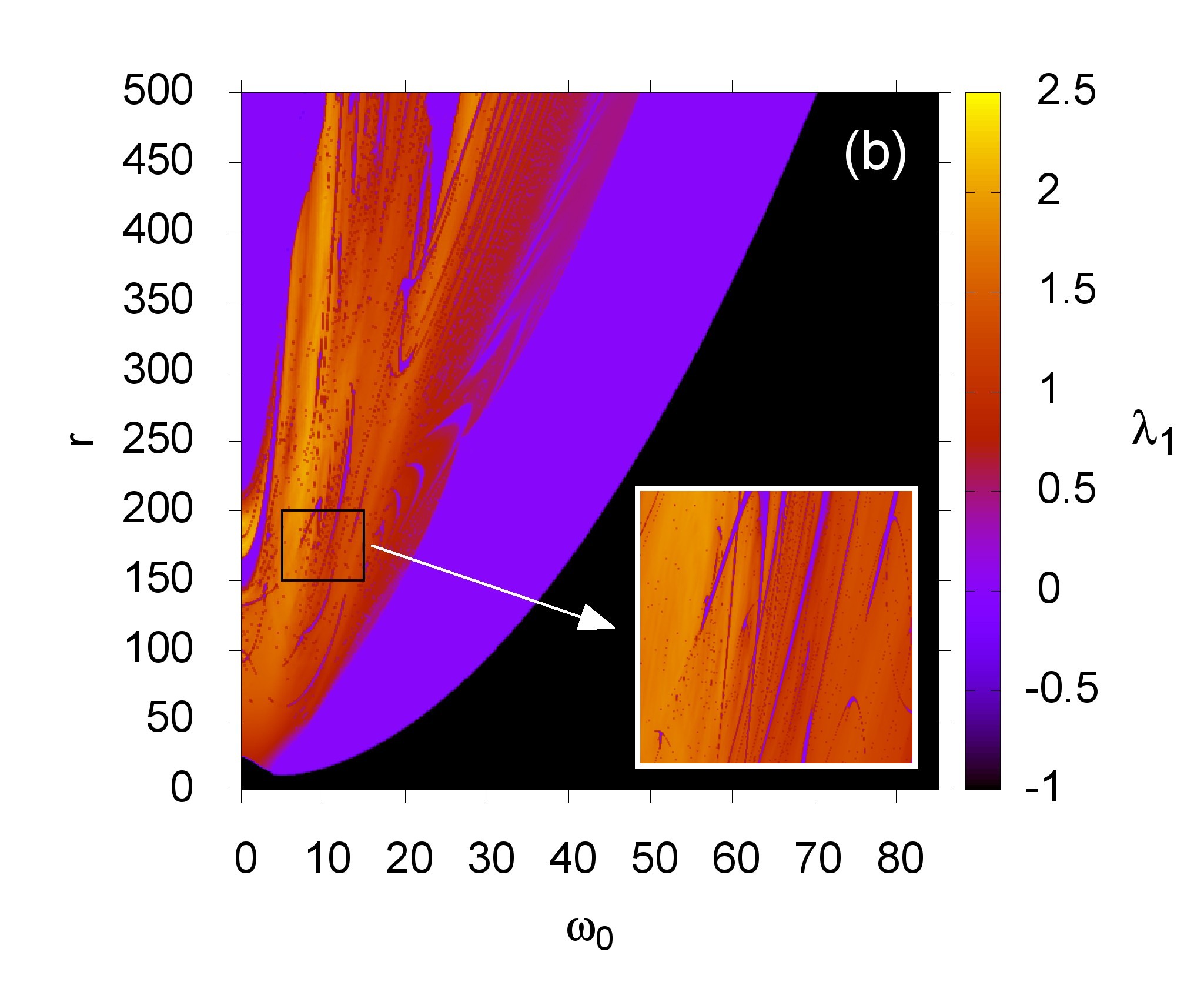
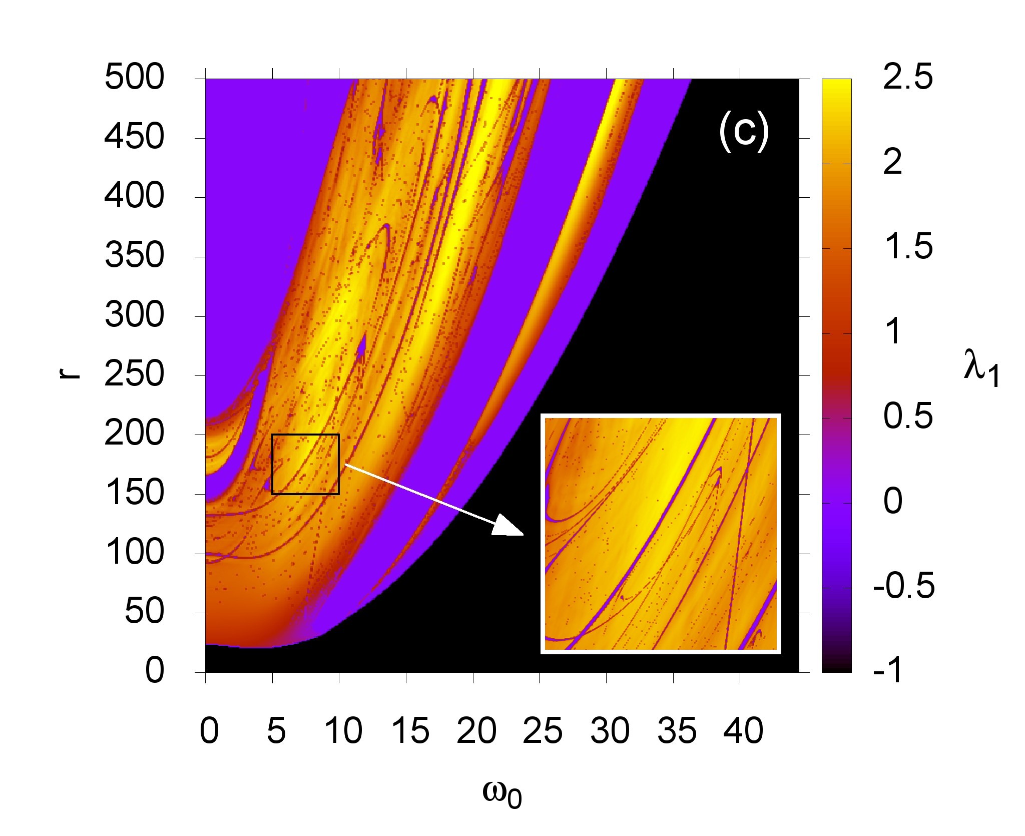
Figure 1: Dependence of the largest Lyapunov exponent $\lambda_{1}$ (color coded) on $\omega_{0}$ and $r$ parameters of the generalized Lorenz model for (a) $\sigma_{\mathrm{m}}=0.1$, (b) $\sigma_{\mathrm{m}}=1$, and (c) $\sigma_{\mathrm{m}}=3$. Other parameters of the system have fixed values: $\sigma=10$, $b=8/3$. Convergence of the solutions of Eqs. (4)–(7) to fixed points ($\lambda_{1}<0$) is shown in black, to periodic solutions ($\lambda_{1}=0$) — in violet/blue color (see the color bar for $\lambda_{1}=0$), to chaotic solutions ($\lambda_{1}>0$) — in a color, consistently with the color bar scale, from violet/blue to yellow. Fine structures are shown in the insets.

In Ref. Macek and Strumik (2010) a single case was studied parametrically: $\sigma_{\mathrm{m}}=1$ and $0<r<50$, which corresponds to the bottom left part of Fig. 1(b). A range of $0<r<500$ in the present study is ten times larger as compared with Ref. Macek and Strumik (2010), which allows us to identify new features of the generalized Lorenz model. The present extended analysis shows that plots for different values of $\sigma_{\mathrm{m}}$ have roughly similar structure. In the right bottom part (where long-term limit cycle oscillations are not possible) solutions converge to fixed points (corresponding to equilibria). Next in the proximity of the diagonal a wide region of periodic (limit cycle) behavior is located, and further toward the left top part of the plots one may find nonperiodic (chaotic) solutions followed by periodic region close to the left top corner. For $\sigma_{\mathrm{m}}=0.1$ and $1$ [Figs. 1(a) and (b)] the “diagonal” region of periodic solutions is homogeneous (without gaps) whereas for $\sigma_{\mathrm{m}}=3$ [Fig. 1(c)] one can see a gap of chaotic solutions dividing this region into two parts. More detailed inspection of the plots reveals complicated structure of regions, where domains of chaotic solutions are intertwined finely with domains of periodic solutions that makes influence of the parameters $\omega_{0}$ and $r$ even more complicated, see insets to Fig. 1. The fine structure in the parameter space is seen for all values of $\sigma_{\mathrm{m}}$ parameter considered here, and it implies interesting properties of the dynamics as regards to regularity of convective motions, when affected by changing boundary conditions related to control parameters $r$ and $\omega_{0}$ used in the model.

As seen in Fig. 1 the dependence of solutions of the system on $\omega_{0}$ parameter (related to $B_{0}$) can be quite complicated. In the simplest case, e.g., for $r=50$, ignoring the fine structure of the chaotic region, for the increasing $\omega_{0}$ parameter we observe a transition from chaotic (through periodic) to fixed point solutions, cf. (Fig. 1 in Macek and Strumik (2010)). This suggests purely damping influence of the increasing external magnetic field. However, for higher values of $r$, e.g., for $r=350$, we rather observe more complex transitions between dynamical regimes: “periodic” – “chaotic” – “periodic” – “fixed point” for $\sigma_{\mathrm{m}}\leq 1$ [Figs. 1(a) and (b)] and “periodic” – “chaotic” – “periodic” – “chaotic” – “periodic” – “fixed point” for $\sigma_{\mathrm{m}}=3$ [Fig. 1(c)].

The external temperature gradient $\delta T$ also influences the dynamics in an intricate manner as one can see in Fig. 1 analyzing the dependence of solutions on $r\propto\delta T$ for fixed values of $\omega_{0}$. Obviously, for $\omega_{0}=0$ we obtain a description fully corresponding to that for classical Lorenz equations of Ref. Lorenz (1963) with the well-known Lorenz strange attractor. This can be easily understood by analysis of Eqs. (4)–(7), where Eq. (7) decouples from the first three equations for $\omega_{0}=0$, which gives classical Lorenz system. In this case the dynamical scenario for increasing $r$ with $\omega_{0}=0$ can be described as the following transition between dynamical regimes: “fixed point” – “chaotic” – “periodic” – “chaotic” – “periodic”. However, for higher values of $\omega_{0}$, e.g., $\omega_{0}=15$ the initial transition from fixed point to chaotic dynamics has an intermediate phase of limit cycle periodic oscillations. Some new strange attractors appearing for the magnetized fluid have been presented in Ref. Macek and Strumik (2010).

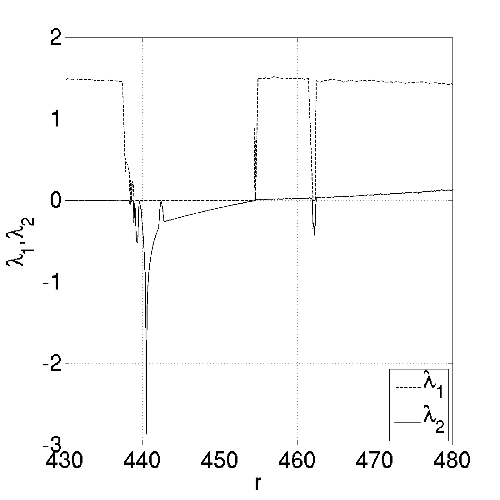
Figure 2: Dependence of the two largest Lyapunov exponents $\lambda_{1}$ (dashed line) and $\lambda_{2}$ (solid line), $\lambda_{1}>\lambda_{2}$, on parameter $r$.

It is even more interesting that in the range $0<r<500$ we have identified hyperchaotic solutions for small values of $\sigma_{\mathrm{m}}$ parameter. Namely, in Fig. 2 we show the dependence of the two largest Lyapunov exponents $\lambda_{1}$ (dashed line) and $\lambda_{2}$ (solid line), $\lambda_{1}>\lambda_{2}$, on the parameter $r$ of the system for $\omega_{0}=5.95$, $\sigma_{\mathrm{m}}=0.1$ with fixed values of the other standard Lorenz system parameters $\sigma=10$, and $b=8/3$. The second Lyapunov exponent $\lambda_{2}$ becomes positive for $r\geq 454.7$, which implies a transition to hyperchaotic dynamics. The largest Lyapunov exponent $\lambda_{1}$ increases abruptly during this transition, whereas the second exponent $\lambda_{2}$ also becomes positive still increasing its value rather smoothly. The region of hyperchaotic behavior has a gap for $461.8<r<462.4$, where periodic solutions appear, see Fig. 2. These results may be of special interest for experimental identification of hyperchaotic dynamics in plasmas. Admittedly, it could rather be difficult to identify such a system in general because any dynamical system exhibiting divergence of trajectories in two directions (with two positive Lyapunov exponents) is clearly more complex than a chaotic system with only one such an unstable direction Rossler (2007). In this context, analysis of statistical properties (e.g. distributions or scaling in intermittency) of the observed dynamical behavior can be more interesting from experimental point of view; thus we discuss the statistics below.

In Ref. Macek and Strumik (2010) some solutions (for $r=28$, $\omega_{0}=4.8$, $\sigma_{\mathrm{m}}=1$) of the dynamical system of Eqs. (4)–(7) have been discussed as examples of type III intermittent behavior. In the present study we extend this analysis to other cases. It is known that the classical Lorenz system exhibits type I intermittency transition from periodic to chaotic dynamics for the value of control parameter $r\approx 166.06$. In fact, in Fig. 1 one can see a branch of periodic-chaotic boundary originating from this point for $\omega_{0}=0$ in the parameter plane. When the magnetic field is taken into account, type I intermittency occurs along this branch, e.g., for $r=256$, $\omega_{0}\approx 3.74$, $\sigma_{\mathrm{m}}=1$.

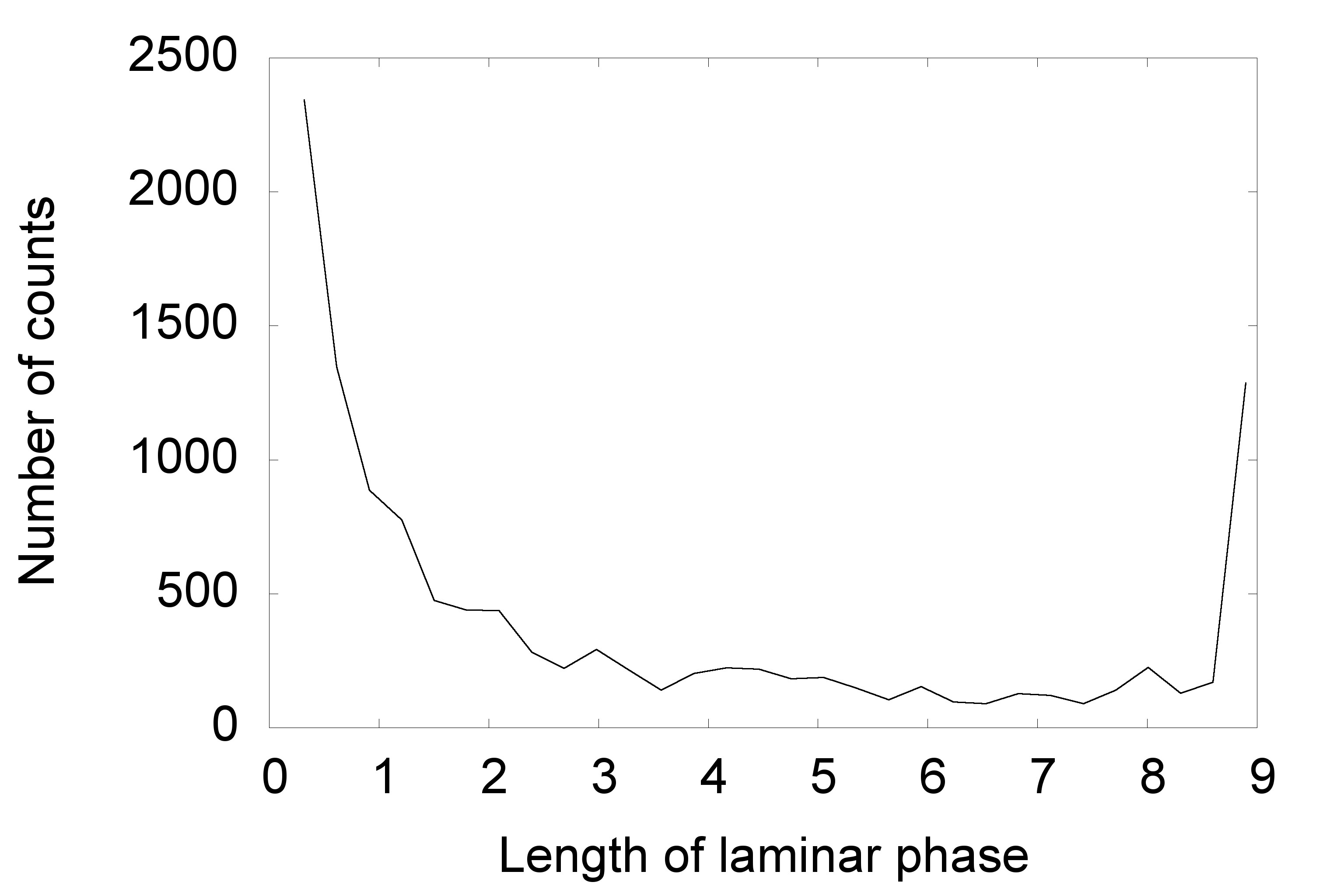
Figure 3: Distribution of the lengths of laminar phases for $r=256$, $\omega_{0}=3.74$, $\sigma_{\mathrm{m}}=1$.

Next, we determine the lengths of laminar phases and their distribution using an algorithm, where pieces of a long numerical solution are compared to a periodic (laminar) phase pattern in four-dimensional phase space. The piecewise numerical solution of Eqs. (4)–(7) is a set of points in the phase space, thus based on the average distance between the points and their nearest neighbors found in the laminar pattern we can identify laminar phases. As demonstrated in Fig. 3 for the type I intermittency with characteristic $U$ shape of the distribution of laminar phases the maximum length of laminar phase has some finite value. Moreover, as shown in Fig. 4 in this case we observe another characteristic attributes of the type I intermittency, namely scaling of the mean length of laminar phase with control parameter $\propto\epsilon^{-1/2}$, where $\epsilon=|\omega_{0}-\omega_{0c}|$.

In conclusion, the four-dimensional dynamical system for convection in a magnetized viscous fluid exhibits quite unusual features depending on the control parameters of the model. It is known that increasing temperature gradient $\delta T$ in the standard Lorenz equations does not imply more chaos in the model Sparrow (1982). Our study provides detailed picture of this counterintuitive influence of $\delta T$ on the generalized Lorenz model, where the system goes through intertwined regions of chaotic, periodic, and fixed-point asymptotic solutions. Quite surprisingly a similar complicated influence is seen for systematic increase of the background magnetic field strength $B_{0}$. The fine structure in the control parameters space clearly shows that the influence of $B_{0}$ is much more intricate than a simple stabilizing effect predicted by simplified analysis of influence of the magnetic field on convective motion discussed in textbooks (see, e.g. Ref. Cowling (1976)). This is interesting because physical circumstances are indeed known where even weak field may have strong destabilizing effect Bajer and Mizerski (2013).

In a chaotic regime but near the border with periodic solutions, in addition to previously identified type III intermittency, we have also observed type I intermittent behavior of the system that could provide new mechanisms of release of kinetic and magnetic energy bursts. It is worth noting that the observed sudden transitions from regular to irregular behavior only mimic stochastic forces, but in fact they result from nonlinearity; i.e., they are due to the disappearance of the fixed points of the dynamical system or owing to a change in their stability.

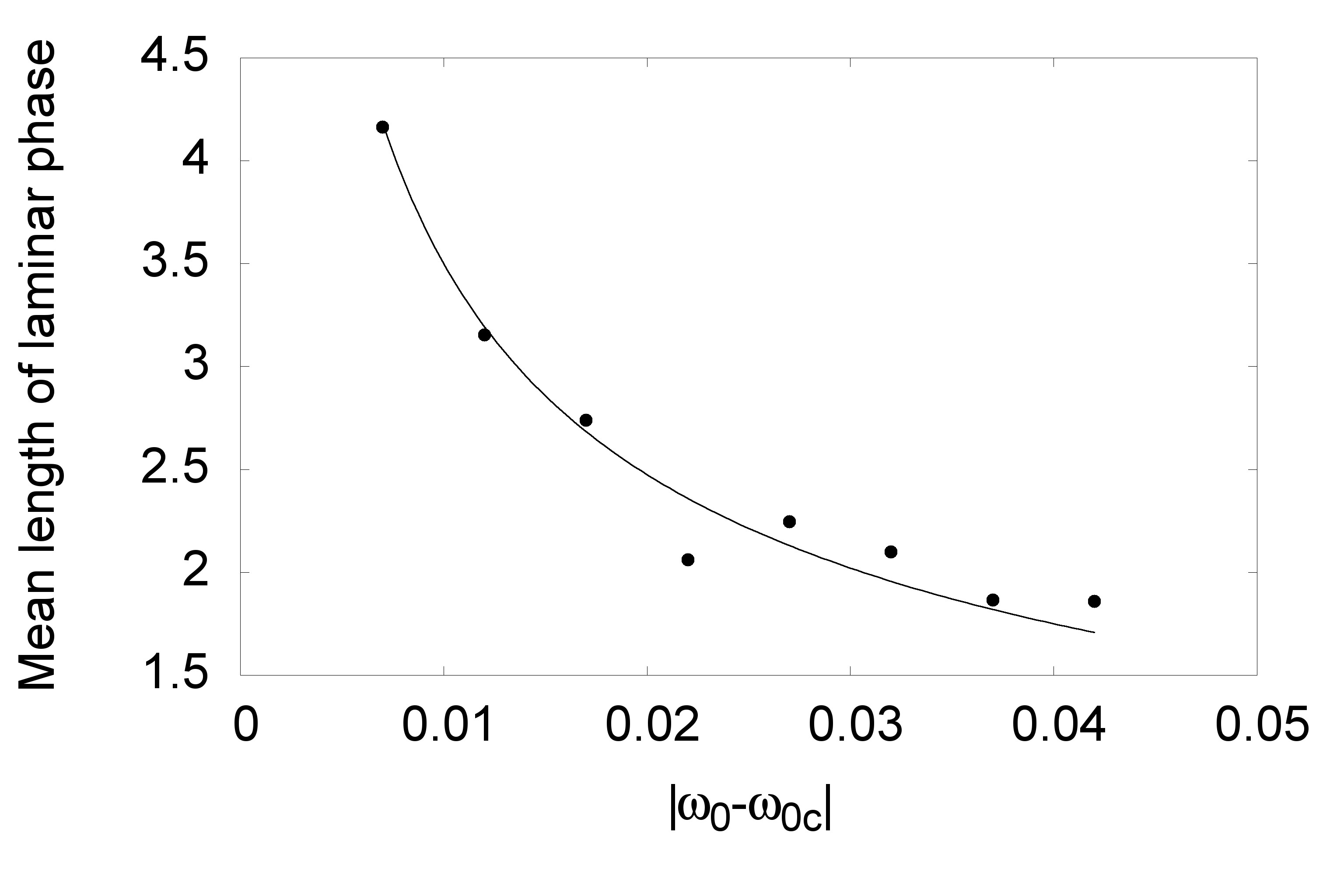
Figure 4: Scaling of the mean length of the laminar phase with control parameter $\epsilon=|\omega_{0}-\omega_{0c}|$ for the case shown in Fig. 3, where $\omega_{0c}$ is a critical value at which intermittency appears.

It is important to note that besides the chaotic behavior well known for the Lorenz model with unmagnetized fluid, we have also identified here for the first time a hyperchaotic dynamics in a magnetic dynamical system, with two positive Lyapunov exponents appearing for some value of the intensity of the applied magnetic field. Admittedly, this new type of chaos is only possible in at least four-dimensional system, hence this results here from the interplay between anisotropic tension of magnetic field lines and magnetic viscosity.

Basically, our analysis focuses on characteristic signatures of the hydromagnetic convection that can be relevant for observational identification of this kind of dynamical behavior, e.g., through analysis of statistical properties of observed intermittent energy bursts as compared with those predicted by the model presented in this Letter. In this context the new hyperchaotic system characterized by both types I and III of intermittent energy release may provide an approximate description of irregular convective dynamical processes observed often in various magnetized plasmas in both laboratory and space, e.g., for solar sunspots Nordlund et al. (2009), planetary and stellar liquid interiors Busse (2000), and possibly for magnetoconfined plasmas in tokamaks Antar et al. (2003), nanodevices and microchannels in nanotechnology.

This work was supported by the National Science Center (NCN) through Grant NN 307 0564 40. W. M. acknowledges support by the European Community’s Seventh Framework Programme ([FP7/2007-2013]) under Grant agreement No. 313038/STORM.

References

- Lorenz (1963) E. N. Lorenz, J. Atmos. Sci. 20, 130 (1963).
- Sparrow (1982) C. Sparrow, The Lorenz Equations: Bifurcations, Chaos and Strange Attractors (Springer-Verlag, Berlin, 1982).
- Macek and Strumik (2010) W. M. Macek and M. Strumik, Phys. Rev. E 82, 027301 (2010).
- Pomeau and Manneville (1980) Y. Pomeau and P. Manneville, Commun. Math. Phys. 74, 189 (1980).
- Rossler (1979) O. E. Rossler, Phys. Lett. A 71, 155 (1979).
- Rossler (2007) C. Letellier and O. E. Rossler, Scholarpedia 2, 1936 (2007).
- Landau et al. (1984) L. D. Landau, E. M. Lifshitz, and L. P. Pitaevskii, Electrodynamics of Continuous Media, (Pergamon Press, Oxford, 1984), vol. 8.
- Lord Rayleigh (1916) Lord Rayleigh, Philos. Mag. 32, 529 (1916).
- Bergé et al. (1984) P. Bergé, Y. Pomeau, and C. Vidal, Order within Chaos. Towards a Deterministic Approach to Turbulence (Wiley, New York, 1984).
- Schuster (1988) H. G. Schuster, Deterministic Chaos. An Introduction (VCH Verlagsgesellschaft, Weinheim, 1988).
- Boussinesq (1903) J. Boussinesq, Théorie Analytique de la Chaleur (Gauthier-Villars, 1903).
- Eckmann and Ruelle (1985) J.-P. Eckmann and D. Ruelle, Rev. Mod. Phys. 57, 617 (1985).
- Cowling (1976) T. G. Cowling, Magnetohydrodynamics (Adam Hilger, Bristol, 1976).
- Bajer and Mizerski (2013) K. Bajer and K. Mizerski, Phys. Rev. Lett. 110, 104503 (2013).
- Nordlund et al. (2009) Å. Nordlund, R. F. Stein, and M. Asplund, Living Rev. Solar Phys. 6, 2 (2009).
- Busse (2000) F. H. Busse, Annu. Rev. Fluid Mech. 32, 383 (2000).
- Antar et al. (2003) G. Y. Antar, G. Counsell, Y. Yu, B. Labombard, and P. Devynck, Phys. Plasmas 10, 419 (2003).