Structured regularization for conditional Gaussian graphical models

Abstract

Conditional Gaussian graphical models (cGGM) are a recent reparametrization of the multivariate linear regression model which explicitly exhibits $i)$ the partial covariances between the predictors and the responses, and $ii)$ the partial covariances between the responses themselves. Such models are particularly suitable for interpretability since partial covariances describe strong relationships between variables. In this framework, we propose a regularization scheme to enhance the learning strategy of the model by driving the selection of the relevant input features by prior structural information. It comes with an efficient alternating optimization procedure which is guaranteed to converge to the global minimum. On top of showing competitive performance on artificial and real datasets, our method demonstrates capabilities for fine interpretation of its parameters, as illustrated on three high-dimensional datasets from spectroscopy, genetics, and genomics.

1 Introduction

Multivariate regression, i.e. regression with multiple response variables, is increasingly used to model high dimensional problems. By considering multiple responses, we wish to strengthen the estimation and/or selection of the relevant input features, by taking advantage of the dependency pattern between the outputs. This is particularly appealing when the data is scarce, or even in the ’$n<p$’ high dimensional setup, in which framework this work enters. Compared to its univariate counterpart, the general linear model aims to predict several – say $q$ – responses from a set of $p$ predictors, relying on a training data set $\left\{(\mathbf{x}_{i},\mathbf{y}_{i})\right\}_{i=1,\dots,n}$:

$$\mathbf{y}_{i}=\mathbf{B}^{T}\mathbf{x}_{i}+\boldsymbol{\varepsilon}_{i},\quad\boldsymbol{\varepsilon}_{i}\sim\mathcal{N}(\mathbf{0},\mathbf{R}),\quad\forall i=1,\dots,n.$$ (1)

The $p\times q$ matrix of regression coefficients $\mathbf{B}$ and the $q\times q$ covariance matrix $\mathbf{R}$ of the Gaussian noise $\boldsymbol{\varepsilon}_{i}$ are unknown. Model (1) has been studied by [22] in the low dimensional case where both ordinary and generalized least squares estimators of $\mathbf{B}$ coincide and do not depend on $\mathbf{R}$. These approaches boil down to performing $q$ independent regressions, each column $\mathbf{B}_{j}$ describing the weights associating the $p$ predictors to the $j$th response. In the $n<p$ setup however, these estimators are not defined.

Mimicking the univariate-output case, multivariate penalized methods aim to regularize the problem by biasing the regression coefficients toward a given feasible set. Sparsity within the set of predictors is usually the most wanted feature in the high-dimensional setting, which can be met in the multivariate framework by a straightforward application of the most popular penalty-based methods from the univariate world involving $\ell_{1}$-regularization. Still, by encouraging sparsity or any other priors by not distinguishing the regression parameters across the outputs, we roughly treat multivariate regression as independent multiple regression problems. It is obviously of the highest interest to treat the problem jointly, so that the structure of the output drives the way the parameters are penalized, and eventually, selected. Several recent papers tackle the multivariate regression problem with penalty-based approaches by including the dependency pattern of the outputs in the learning process. When this pattern is known a priori, we enter the “multitask” framework where many authors have suggested variants of the $\ell_{1}$-penalty shaped accordingly. A natural approach is to encourage a similar behavior of the regression parameters across the outputs – or tasks – using group-norms zeroing a full row of $\mathbf{B}$ at once, across the corresponding outputs (see, e.g., [3, 25]). Refinements exist to cope with complex dependency structures, using graph or tree structures ([13, 14]), yet the pattern between the responses remains fixed. When it is unknown, the general linear model (1) is a natural tool to account for dependencies between the responses. In this vein, [30, 42] suggest penalizing the negative log-likelihood of (1) by two $\ell_{1}$ norms respectively inducing sparsity on the regression coefficients $\mathbf{B}$ and on the inverse covariance $\mathbf{R}^{-1}$. Theoretical guarantees are proposed in [18], with a two-stage procedure involving a plug-in estimator of the inverse covariance, which leads to a computationally less demanding optimization procedure. However their criterion is hard to minimize as it is only bi-convex in $(\mathbf{B},\mathbf{R}^{-1})$, and no theoretical guarantee is provided regarding the convergence of the proposed optimization strategy.

In [33, 43], an elegant re-parametrization of (1) is depicted, leading to a formulation that is jointly convex and enjoys features of Gaussian Graphical Models (GGM). This has been referred to as a ’conditional Gaussian Graphical Model’ (cGGM) or ’partial Gaussian Graphical Model’ in the recent literature. A remarkable feature of this formulation is to explicitly exhibit the direct relationships that exist between the predictors $\mathbf{x}_{i}$ and the responses $\mathbf{y}_{i}$ through their partial covariances (denoted $\boldsymbol{\Omega}_{\mathbf{x}\mathbf{y}}$ hereafter). Dealing with the direct links $\boldsymbol{\Omega}_{\mathbf{x}\mathbf{y}}$ is much more convenient for interpretability than is dealing with the regression parameters $\mathbf{B}$, the latter entailing both direct and indirect influences, possibly due to some strong correlations between the responses. Regarding the learning strategy, [33] propose to regularize the cGGM log-likelihood by two $\ell_{1}$-norms respectively acting on the partial covariances between the features and the responses $\boldsymbol{\Omega}_{\mathbf{x}\mathbf{y}}$ on the first hand, and on the partial covariance between the responses themselves via $\mathbf{R}^{-1}$ on the second hand.

In this paper, we build on this approach yet in a slightly different setting. First we typically assume a reasonable number of outputs compared to the number of predictors and sample size (while we insist on the fact that the number of predictors may exceed the sample size). As a consequence our regularizer induces sparsity on the direct relationships like in [33], yet no sparsity assumption is made for the inverse covariance. Second, we consider applications where structural information about sparsity is available. Here the structural information will be embedded in the regularization scheme via an additional regularization term using an application-specific metrics, in the same manner as in the ’structured’ versions of the Elastic-net [32, 11, 21], or quadratic penalty function using the Laplacian graph [29, 19] proposed in the univariate-output case. We show that the resulting penalized likelihood optimization problem can be solved efficiently and provide algorithmic convergence guarantees for the two-step procedure presented here. Penalized criteria for the choice of the regularization parameters are also provided. We also investigate the importance of embedding for structural prior information in the various contexts of spectroscopy, genomic selection and regulatory motif discovery, illustrating how accounting for application-specific improves both performance and interpretability. The procedure is available as an R-package called spring, available on the R-forge.

The outline of the paper is as follows. In Section 2 we provide background on cGGM and present our regularization scheme. In Section 3, we develop an efficient optimization strategy in order to minimize the associated criterion. A paragraph also addresses the model selection issue. Section 4 is dedicated to illustrative simulation studies. In Section 5, we investigate three multivariate data sets: first, we consider an example in spectrometry with the analysis of cookie dough samples; second, the relationships between genetic markers and a series of phenotypes of the plant Brassica napus is addressed; and third, we investigate the discovery of regulatory motifs of yeast from time-course microarray experiments. In these applications, some specific underlying structuring priors arise, the integration of which within our model is detailed as it is one of the main contributions of our work.

2 Model setup

2.1 Background on cGGM

The statistical framework of cGGM arises from a different parametrization of (1) which fills the gap between multivariate regression and GGM. It extends to the multivariate case the links existing between the linear model, partial correlations and GGM, as depicted for instance by [24] then [28]. To the best of our knowledge, the connection in the case of multiple reponses was first underlined by [33], which we recall here. It amounts to investigating the joint probability distribution of $(\mathbf{x}_{i},\mathbf{y}_{i})$ in the Gaussian case, with the following block-wise decomposition of the covariance matrix ${\boldsymbol{\Sigma}}$ and its inverse $\boldsymbol{\Omega}={\boldsymbol{\Sigma}}^{-1}$:

$${\boldsymbol{\Sigma}}=\begin{pmatrix}{\boldsymbol{\Sigma}}_{\mathbf{x}\mathbf{x}}&{\boldsymbol{\Sigma}}_{\mathbf{x}\mathbf{y}}\\ {\boldsymbol{\Sigma}}_{\mathbf{y}\mathbf{x}}&{\boldsymbol{\Sigma}}_{\mathbf{y}\mathbf{y}}\\ \end{pmatrix},\quad\boldsymbol{\Omega}=\begin{pmatrix}\boldsymbol{\Omega}_{\mathbf{x}\mathbf{x}}&\boldsymbol{\Omega}_{\mathbf{x}\mathbf{y}}\\ \boldsymbol{\Omega}_{\mathbf{y}\mathbf{x}}&\boldsymbol{\Omega}_{\mathbf{y}\mathbf{y}}\\ \end{pmatrix}.$$ (2)

Back to the distribution of $\mathbf{y}_{i}$ conditional on $\mathbf{x}_{i}$, multivariate Gaussian analysis shows that, for centered $\mathbf{x}_{i}$ and $\mathbf{y}_{i}$,

$$\mathbf{y}_{i}|\mathbf{x}_{i}\sim\mathcal{N}\left(-\boldsymbol{\Omega}^{-1}_{\mathbf{y}\mathbf{y}}\boldsymbol{\Omega}_{\mathbf{y}\mathbf{x}}\mathbf{x}_{i},\boldsymbol{\Omega}_{\mathbf{y}\mathbf{y}}^{-1}\right).$$ (3)

This model, associated with the full sample $\{(\mathbf{x}_{i},\mathbf{y}_{i})\}_{i=1,\dots,n}$, can be written in a matrix form by stacking in rows first the observations of the responses, and then of the predictors, in two data matrices $\mathbf{Y}$ and $\mathbf{X}$ with respective sizes $n\times q$ and $n\times p$, such that

$$\mathbf{Y}=-\mathbf{X}\boldsymbol{\Omega}_{\mathbf{x}\mathbf{y}}\boldsymbol{\Omega}_{\mathbf{y}\mathbf{y}}^{-1}+\boldsymbol{\varepsilon},\\ \mathrm{vec}(\boldsymbol{\varepsilon})\sim\mathcal{N}\left(\mathbf{0}_{nq},\mathbf{I}_{n}\otimes\boldsymbol{\Omega}_{\mathbf{y}\mathbf{y}}^{-1}\right),$$ (4)

where, for a $n\times p$ matrix ${\bf A}$, denoting ${\bf A}_{j}$ its $j$th column, the $\mathrm{vec}$ operator is defined as $\mathrm{vec}({\bf A})=(\mathbf{A}_{1}^{T}\dots\mathbf{A}_{p}^{T})^{T}$. The log-likelihood of (4) – which is a conditional likelihood regarding the joint model (2) – is written

$$\log L(\boldsymbol{\Omega}_{\mathbf{x}\mathbf{y}},\boldsymbol{\Omega}_{\mathbf{y}\mathbf{y}})=\frac{n}{2}\log\left|\boldsymbol{\Omega}_{\mathbf{y}\mathbf{y}}\right|+\\ \frac{n}{2}\mathrm{tr}\left(\left(\mathbf{Y}+\mathbf{X}\boldsymbol{\Omega}_{\mathbf{x}\mathbf{y}}\boldsymbol{\Omega}_{\mathbf{y}\mathbf{y}}^{-1}\right)\boldsymbol{\Omega}_{\mathbf{y}\mathbf{y}}\left(\mathbf{Y}+\mathbf{X}\boldsymbol{\Omega}_{\mathbf{x}\mathbf{y}}\boldsymbol{\Omega}_{\mathbf{y}\mathbf{y}}^{-1}\right)^{T}\right)+\mathrm{cst.}$$ (5)

$\mathbf{R}_{\text{low}}$ $\mathbf{R}_{\text{med}}$ $\mathbf{R}_{\text{high}}$ $\boldsymbol{\Omega}_{\mathbf{x}\mathbf{y}}$ $\mathbf{B}_{\text{low}}$ $\mathbf{B}_{\text{med}}$ $\mathbf{B}_{\text{high}}$	$\mathbf{R}_{\text{low}}$ $\mathbf{R}_{\text{med}}$ $\mathbf{R}_{\text{high}}$ $\boldsymbol{\Omega}_{\mathbf{x}\mathbf{y}}$ $\mathbf{B}_{\text{low}}$ $\mathbf{B}_{\text{med}}$ $\mathbf{B}_{\text{high}}$
(a)	(b)

Figure 1: Toy examples to illustrate the relationships between $\mathbf{B},\boldsymbol{\Omega}_{\mathbf{x}\mathbf{y}}$ and $\mathbf{R}$ in the cGGM (better seen in color): on panel $a)$, a situation with no particular structure among the predictors; on panel $b)$, a strong neighborhood structure. For each panel, we represent the effect of stronger correlations in $\mathbf{R}$ on masking the direct links in $\mathbf{B}$.

Introducing the empirical matrices of covariance $\mathbf{S}_{\mathbf{y}\mathbf{y}}=n^{-1}\sum_{i=1}^{n}\mathbf{y}_{i}\mathbf{y}_{i}^{T}$, $\mathbf{S}_{\mathbf{x}\mathbf{x}}=n^{-1}\sum_{i=1}^{n}\mathbf{x}_{i}\mathbf{x}_{i}^{T}$, and $\mathbf{S}_{\mathbf{y}\mathbf{x}}=n^{-1}\sum_{i=1}^{n}\mathbf{y}_{i}\mathbf{x}_{i}^{T}$, one has

$$-\frac{2}{n}\log L(\boldsymbol{\Omega}_{\mathbf{x}\mathbf{y}},\boldsymbol{\Omega}_{\mathbf{y}\mathbf{y}})=-\log\left|\boldsymbol{\Omega}_{\mathbf{y}\mathbf{y}}\right|+\mathrm{tr}\left(\mathbf{S}_{\mathbf{y}\mathbf{y}}\boldsymbol{\Omega}_{\mathbf{y}\mathbf{y}}\right)\\ +2\mathrm{tr}\left(\mathbf{S}_{\mathbf{x}\mathbf{y}}\boldsymbol{\Omega}_{\mathbf{y}\mathbf{x}}\right)+\mathrm{tr}(\boldsymbol{\Omega}_{\mathbf{y}\mathbf{x}}\mathbf{S}_{\mathbf{x}\mathbf{x}}\boldsymbol{\Omega}_{\mathbf{x}\mathbf{y}}\boldsymbol{\Omega}_{\mathbf{y}\mathbf{y}}^{-1})+\mathrm{cst.}$$ (6)

We notice by comparing the cGGM (3) to the multivariate regression model (1) that $\boldsymbol{\Omega}_{\mathbf{y}\mathbf{y}}^{-1}=\mathbf{R}\text{ and }\mathbf{B}=-\boldsymbol{\Omega}_{\mathbf{x}\mathbf{y}}\boldsymbol{\Omega}_{\mathbf{y}\mathbf{y}}^{-1}$. Although equivalent to (1), the alternative parametrization (3) shows two important differences with several implications. First, in light of convex optimization theory, the negative log-likelihood (5) can be shown to be jointly convex in $(\boldsymbol{\Omega}_{\mathbf{x}\mathbf{y}},\boldsymbol{\Omega}_{\mathbf{y}\mathbf{y}})$ (a formal proof can be found in [43]). Minimization problems involving (5) will thus be amenable to a global solution, which facilitates both optimization and theoretical analysis. As such, the conditional negative log-likelihood (5) will serve as a building block for our learning criterion. Second, it unveils new interpretations for the relationships between input and output variables, as discussed in [33]: $\boldsymbol{\Omega}_{\mathbf{x}\mathbf{y}}$ describes the direct relationships between predictors and responses, the support of which we are looking for to select relevant interactions. On the other hand, $\mathbf{B}$ entails both direct and indirect influences, possibly due to some strong correlations between the responses, described by the covariance matrix $\mathbf{R}$ (or equivalently its inverse $\boldsymbol{\Omega}_{\mathbf{y}\mathbf{y}}$). To provide additional insights on cGGM, Figure 1 illustrates the relationships between $\mathbf{B},\boldsymbol{\Omega}_{\mathbf{x}\mathbf{y}}$ and $\mathbf{R}$ in two simple scenarios where $p=40$ and $q=5$. Scenarios $a)$ and $b)$ are discriminated by the presence of a strong structure among the predictors. Still, the important point to grasp at this stage of the paper is how strong correlations between outcomes can completely “mask” the direct links in the regression coefficients: the stronger the correlation in $\mathbf{R}$, the less it is possible to distinguish in $\mathbf{B}$ the non-zero coefficients of $\boldsymbol{\Omega}_{\mathbf{x}\mathbf{y}}$.

2.2 Structured regularization with underlying sparsity

Our regularization scheme starts by considering some structural prior information about the relationships between the coefficients. We are typically thinking of a situation where similar inputs are expected to have similar direct relationships with the outputs. The right panel of Figure 1 represents an illustration of such a situation, where there exists an extreme neighborhood structure between the predictors. This depicts a pattern that acts along the rows of $\mathbf{B}$ or $\boldsymbol{\Omega}_{\mathbf{x}\mathbf{y}}$ as substantiated by the following Bayesian point of view.

Bayesian interpretation

Suppose that the similarities can be encoded into a matrix $\mathbf{L}$. Our aim is to account for this information when learning the coefficients. The Bayesian framework provides a convenient setup for defining the way the structural information should be accounted for. In the single output case (see, e.g. [23]), a conjugate prior for $\boldsymbol{\beta}$ would be $\mathcal{N}(\mathbf{0},\mathbf{L}^{-1})$. Combined with the covariance between the outputs, this gives

$$\mathrm{vec}(\mathbf{B})\sim\mathcal{N}(\mathbf{0},\mathbf{R}\otimes\mathbf{L}^{-1}),$$

where $\otimes$ is the Kronecker product. By properties of the $\mathrm{vec}$ operator, this can be stated straightforwardly as

$$\mathrm{vec}(\boldsymbol{\Omega}_{\mathbf{x}\mathbf{y}})\sim\mathcal{N}(\mathbf{0},\mathbf{R}^{-1}\otimes\mathbf{L}^{-1})$$

for the direct links. Choosing such a prior results in

$$\log\mathbb{P}(\boldsymbol{\Omega}_{\mathbf{x}\mathbf{y}}|\mathbf{L},\mathbf{R})=\frac{1}{2}\mathrm{tr}\left(\boldsymbol{\Omega}_{\mathbf{x}\mathbf{y}}^{T}\mathbf{L}\boldsymbol{\Omega}_{\mathbf{x}\mathbf{y}}\mathbf{R}\right)+\mathrm{cst.}$$

Criterion

Through this argument, we propose a criterion with two terms to regularize the conditional negative log-likelihood (5): first, a smooth trace term relying on the available structural information $\mathbf{L}$; and second, an $\ell_{1}$ norm that encourages sparsity among the direct links. We write the criterion as a function of $(\boldsymbol{\Omega}_{\mathbf{x}\mathbf{y}},\boldsymbol{\Omega}_{\mathbf{y}\mathbf{y}})$ rather than $(\boldsymbol{\Omega}_{\mathbf{x}\mathbf{y}},\mathbf{R})$, although equivalent in terms of estimation, since the former leads to a convex formulation. The optimization problem turns to the minimization of

$$J(\boldsymbol{\Omega}_{\mathbf{x}\mathbf{y}},\boldsymbol{\Omega}_{\mathbf{y}\mathbf{y}})=-\frac{1}{n}\log L(\boldsymbol{\Omega}_{\mathbf{x}\mathbf{y}},\boldsymbol{\Omega}_{\mathbf{y}\mathbf{y}})\\ +\frac{\lambda_{2}}{2}\mathrm{tr}\left(\boldsymbol{\Omega}_{\mathbf{y}\mathbf{x}}\mathbf{L}\boldsymbol{\Omega}_{\mathbf{x}\mathbf{y}}\boldsymbol{\Omega}_{\mathbf{y}\mathbf{y}}^{-1}\right)+\lambda_{1}\|\boldsymbol{\Omega}_{\mathbf{x}\mathbf{y}}\|_{1}.$$ (7)

2.3 Connection to other sparse methods

To get more insight into our model and to facilitate connections with existing approaches, we shall write the objective function (7) as a penalized univariate regression problem. This amounts to “vectorizing” model (4) with respect to $\boldsymbol{\Omega}_{\mathbf{x}\mathbf{y}}$, i.e., to writing the objective as a function of $(\boldsymbol{\omega},\boldsymbol{\Omega}_{\mathbf{y}\mathbf{y}})$ where $\boldsymbol{\omega}=\mathrm{vec}(\boldsymbol{\Omega}_{\mathbf{x}\mathbf{y}})$. This is stated in the following proposition, which can be derived from straightforward matrix algebra, as proved in Appendix Section A.1. The main interest of this proposition will become clear when deriving the optimization procedure that aims at minimizing (7), as the optimization problem when $\boldsymbol{\Omega}_{\mathbf{y}\mathbf{y}}$ is fixed turns to a generalized Elastic-Net problem. Note that we use $\mathbf{A}^{1/2}$ to denote the square root of a matrix, obtained for instance by a Cholesky factorization in the case of a symmetric positive definite matrix.

Proposition 1.

Let $\boldsymbol{\omega}=\mathrm{vec}(\boldsymbol{\Omega}_{\mathbf{x}\mathbf{y}})$. An equivalent vector form of (7) is

$$J(\boldsymbol{\omega},\boldsymbol{\Omega}_{\mathbf{y}\mathbf{y}})=-\frac{1}{2}\log|\boldsymbol{\Omega}_{\mathbf{y}\mathbf{y}}|+\frac{1}{2n}\left\|\tilde{\mathbf{y}}+\tilde{\mathbf{X}}\boldsymbol{\omega}\right\|_{2}^{2}\\ +\frac{\lambda_{2}}{2}\boldsymbol{\omega}^{T}\left(\boldsymbol{\Omega}_{\mathbf{y}\mathbf{y}}^{-1}\otimes\mathbf{L}\right)\boldsymbol{\omega}+\lambda_{1}\left\|\boldsymbol{\omega}\right\|_{1},$$

where the $n\times q$ dimensional vector $\tilde{\mathbf{y}}$ and the $nq\times pq$ dimensional matrix $\tilde{\mathbf{X}}$ depends on $\boldsymbol{\Omega}_{\mathbf{y}\mathbf{y}}$ such that

$$\tilde{\mathbf{y}}=\mathrm{vec}(\mathbf{Y}\boldsymbol{\Omega}_{\mathbf{y}\mathbf{y}}^{1/2}),\quad\tilde{\mathbf{X}}=\left(\boldsymbol{\Omega}_{\mathbf{y}\mathbf{y}}^{-1/2}\otimes\mathbf{X}\right).$$

When there is only one response ($q=1$) the variance-covariance matrix $\mathbf{R}$ and its inverse $\boldsymbol{\Omega}_{\mathbf{y}\mathbf{y}}$ turns to a scalar denoted by $\sigma^{2}$, the matrix $\mathbf{B}$ to a $p$-vector $\boldsymbol{\beta}$, and the objective (7) can be rewritten

$$\log(\sigma)+\frac{1}{2n\sigma^{2}}\left\|\mathbf{y}-\mathbf{X}\boldsymbol{\beta}\right\|_{2}^{2}+\frac{\lambda_{2}}{2\sigma^{2}}\boldsymbol{\beta}^{T}\mathbf{L}\boldsymbol{\beta}+\frac{\lambda_{1}}{\sigma^{2}}\|\boldsymbol{\beta}\|_{1}.$$ (8)

We recognize in (8) the log-likelihood of a “usual” linear model with Gaussian noise, unknown variance $\sigma^{2}$ and regression parameters $\boldsymbol{\beta}$, plus a mixture of $\ell_{1}$ and $\ell_{2}$ norms. Assuming that $\sigma$ is known, we recognize the general structured Elastic-net regression. If $\sigma$ is unknown, letting $\lambda_{2}=0$ in (8) leads to the $\ell_{1}$-penalized mixture regression model proposed by [34], where both $\boldsymbol{\beta}$ and $\sigma^{2}$ are inferred. In [34], the authors insist on the importance of penalizing the vector of coefficients by an amount that is inversely proportional to $\sigma$: in the closely related Bayesian Lasso framework of [27], the prior on $\boldsymbol{\beta}$ is defined conditionally on $\sigma$ to guarantee an unimodal posterior.

3 Learning

3.1 Optimization

In the classical framework of parametrization (1), alternate strategies where optimization is successively performed over $\boldsymbol{\Omega}_{\mathbf{x}\mathbf{y}}$ and $\boldsymbol{\Omega}_{\mathbf{y}\mathbf{y}}$ have been proposed [30, 42]. They come with no guarantee of convergence to the global optimum since the objective is only bi-convex. In the cGGM framework of [33, 43], the optimized criterion is jointly convex yet no convergence result is provided regarding the optimization procedure proposed by the authors. Here we also consider the alternate strategy for which theoretical guarantees are provided by the following theorem:

Theorem 1.

Let $n\geq q$. Criterion (7) is jointly convex in $(\boldsymbol{\Omega}_{\mathbf{x}\mathbf{y}},\boldsymbol{\Omega}_{\mathbf{y}\mathbf{y}})$. Moreover, the alternate optimization

$$\hat{\boldsymbol{\Omega}}_{\mathbf{y}\mathbf{y}}^{(k+1)}=\mathop{\mathrm{arg\ min}}_{\boldsymbol{\Omega}_{\mathbf{y}\mathbf{y}}\succ 0}J_{\lambda_{1}\lambda_{2}}(\hat{\boldsymbol{\Omega}}_{\mathbf{x}\mathbf{y}}^{(k)},\boldsymbol{\Omega}_{\mathbf{y}\mathbf{y}}),$$ (9a)

$$\hat{\boldsymbol{\Omega}}_{\mathbf{x}\mathbf{y}}^{(k+1)}=\mathop{\mathrm{arg\ min}}_{\boldsymbol{\Omega}_{\mathbf{x}\mathbf{y}}}J_{\lambda_{1}\lambda_{2}}(\boldsymbol{\Omega}_{\mathbf{x}\mathbf{y}},\hat{\boldsymbol{\Omega}}_{\mathbf{y}\mathbf{y}}^{(k+1)}).$$ (9b)

leads to the optimal solution.

The proof is given in Appendix A.3, and relies on the fact that efficient procedures exist to solve the two convex sub-problems (9a) and (9b).

Because our procedure relies on alternating optimization, it is difficult to give either a global rate of convergence or a complexity bound. Nevertheless, the complexity of each iteration is easy to derive, since it amounts to two well-known problems: the main computational cost in (9a) is due to the SVD of a $q\times q$ matrix, which costs $\mathcal{O}(q^{3})$. Concerning (9b), it amounts to the resolution of an Elastic-Net problem with $p\times q$ variables and $n\times q$ samples. If the final number of nonzero entries in $\hat{\boldsymbol{\Omega}}_{\mathbf{x}\mathbf{y}}$ is $k$, a good implementation with Cholesky update/downdate is roughly in $\mathcal{O}(npq^{2}k)$ (see, e.g. [1]). Since we typically assumed that $p\geq n\geq q$, the global cost of a single iteration of the alternating scheme is thus $\mathcal{O}(npq^{2}k)$, and we theoretically can treat problems with large $p$ when $k$ remains moderate.

Finally, we typically want to compute a series of solutions along the regularization path of Problem (7), i.e. for various values of $(\lambda_{1},\lambda_{2})$. To this end, we simply choose a grid of penalties $\Lambda_{1}\times\Lambda_{2}=\left\{\lambda_{1}^{\text{min}},\dots,\lambda_{1}^{\text{max}}\right\}\times\left\{\lambda_{2}^{\text{min}},\dots,\lambda_{2}^{\text{max}}\right\}$. The process is easily distributed on different computer cores, each core corresponding to a value picked in $\Lambda_{2}$. Then on each core – i.e. for a fix $\lambda_{2}\in\Lambda_{2}$ – we cover all the values of $\lambda_{1}\in\Lambda_{1}$ relying on the warm start strategy frequently used to go through the regularization path of $\ell_{1}$-penalized problems.

3.2 Model selection and parameter tuning

Model selection amounts here to choosing a couple of tuning parameters $(\lambda_{1},\lambda_{2})$ among the grid $\Lambda_{1}\times\Lambda_{2}$, where $\lambda_{1}$ tunes the sparsity while $\lambda_{2}$ tunes the amount of structural regularization. We aim to pick either the model with minimum prediction error, or the one closest to the true model, assuming Equation (3) holds. These two perspectives generally do not lead to the same model choices: when looking for the model minimizing the prediction error, $K$-fold cross-validation is the recommended option ( [12]) despite its additional computational cost. Letting $\kappa:\left\{1,\dots,n\right\}\to\left\{1,\dots,K\right\}$ the function indexing the fold to which observation $i$ is allocated, the CV-choices for $(\lambda_{1}^{\text{cv}},\lambda_{2}^{\text{cv}})$ are the ones that minimize

$$\frac{1}{n}\sum_{i=1}^{n}\left\|\mathbf{x}_{i}^{T}\hat{\mathbf{B}}_{-\kappa(i)}^{\lambda_{1},\lambda_{2}}-\mathbf{y}_{i}\right\|_{2}^{2},$$

where $\hat{\mathbf{B}}_{-\kappa(i)}^{\lambda_{1},\lambda_{2}}$ minimizes the objective (7), once data $\kappa(i)$ has been removed. In place of the prediction error, other quantities can be cross-validated in our context, e.g. the negative log-likelihood (5). In the remainder of the paper, however, we only consider cross-validating the prediction error, though.

As an alternative to cross-validation, penalyzed criteria provide a fast way to perform model selection and are sometimes more suited to the selection of the true underlying model. Although relying on asymptotic derivations, they often offer good practical performance when the sample size $n$ is not too small compared to the problem dimension. For penalized methods, a general form for various information criteria is expressed as a function of the likelihood $L$ (defined by (5) here) and the effective degrees of freedom:

$$-2\log L(\hat{\boldsymbol{\Omega}}^{\lambda_{1},\lambda_{2}}_{\mathbf{x}\mathbf{y}},\hat{\boldsymbol{\Omega}}^{\lambda_{1},\lambda_{2}}_{\mathbf{y}\mathbf{y}})+\mathrm{pen}\cdot\mathrm{df}_{\lambda_{1},\lambda_{2}}.$$

Setting $\text{pen}=2$ or $\log(n)$ respectively leads to AIC or BIC. For the practical evaluation of (3.2), we must give some sense to the effective degrees of freedom $\text{df}_{\lambda_{1},\lambda_{2}}$. We use the now classical definition of [5] and rely on the work of [39] to derive the following Proposition, the proof of which is postponed to Appendix Section A.4.

Proposition 2.

An unbiased estimator of $\text{df}_{\lambda_{1},\lambda_{2}}$ for our fitting procedure is

$$\hat{\mathrm{df}}_{\lambda_{1},\lambda_{2}}=\mathrm{card}(\mathcal{A})\\ -\lambda_{2}\mathrm{tr}\left((\hat{\mathbf{R}}\otimes\mathbf{L})_{\mathcal{A}\mathcal{A}}\left((\hat{\mathbf{R}}\otimes(\mathbf{S}_{\mathbf{x}\mathbf{x}}+\lambda_{2}\mathbf{L}))_{\mathcal{A}\mathcal{A}}\right)^{-1}\right),$$

where $\mathcal{A}=\left\{j:\mathrm{vec}\left(\hat{\boldsymbol{\Omega}}_{\mathbf{x}\mathbf{y}}^{\lambda_{1},\lambda_{2}}\right)\neq 0\right\}$ is the set of nonzero entries in $\hat{\boldsymbol{\Omega}}_{\mathbf{x}\mathbf{y}}^{\lambda_{1},\lambda_{2}}$.

Note that we can compute this expression at no additional cost, relying on computations already made during the optimization process.

4 Simulation studies

In this section, we would like to illustrate the new features of our proposal compared to several baselines in well controlled settings. To this end, we perform two simulation studies to evaluate $i)$ the gain brought by the estimation of the residual covariance $\mathbf{R}$ and $ii)$ the gain brought by the inclusion of informative structure on the predictors via $\mathbf{L}$.

Implementation details

In our experiments, performance are compared with well-established regularization methods, whose implementation is easily accessible: the LASSO ([36]), the multitask group-LASSO, MRCE ([30]), the Elastic-Net ([44]) and the Structured Elastic-Net ([32]). LASSO and group-LASSO are fitted with the R-package glmnet ([7]) and MRCE with [30]’s package. All other methods are fitted using our own code. Our own procedure is available as an R-package called spring, distributed on the R-forge. As such, we sometimes refer to our method as ’SPRING’ in the simulation part.

Data generation

Artificial datasets are generated according to the multivariate regression model (1). We assume that the decomposition $\mathbf{B}=\boldsymbol{\Omega}_{\mathbf{x}\mathbf{y}}\boldsymbol{\Omega}_{\mathbf{y}\mathbf{y}}^{-1}=\boldsymbol{\Omega}_{\mathbf{x}\mathbf{y}}\mathbf{R}$ holds for the regression coefficients. We control the sparsity pattern of $\boldsymbol{\Omega}_{\mathbf{x}\mathbf{y}}$ by arranging non null entries according to a possible structure of the predictors along the rows of $\boldsymbol{\Omega}_{\mathbf{x}\mathbf{y}}$. We always use uncorrelated Gaussian predictors $\mathbf{x}_{i}\sim\mathcal{N}(\mathbf{0},\mathbf{I})$ in order not to promote excessively the methods that take this structure into account. Strength of the relationships between the outputs are tuned by the covariance matrix $\mathbf{R}$. We measure the performance of the learning procedures thanks to the prediction error (PE) estimated using a large test set of observations generated according to the true model. When relevant, mean squared error (MSE) of the regression coefficients $\mathbf{B}$ is also presented. For conciseness, it is eluded when it shows results which are quantitatively identical to PE.

4.1 Influence of covariance between outcomes

The first simulation study aims to illustrate the advantage of splitting $\mathbf{B}$ into $-\boldsymbol{\Omega}_{\mathbf{x}\mathbf{y}}\mathbf{R}$ over working directly on $\mathbf{B}$. We set $p=40$ predictors, $q=5$ outcomes and randomly select $25$ non null entries in $\left\{-1,1\right\}$ to fill $\boldsymbol{\Omega}_{\mathbf{x}\mathbf{y}}$. We do not put any structure along the predictors as this study intends to measure the gain of using the cGGM approach. The covariance follows a Toeplitz scheme: one has $\mathbf{R}_{ij}=\tau^{|i-j|}$, for $i,j=1,\dots,q$. We consider three scenarios tuned by $\tau\in\left\{.1,.5,.9\right\}$ corresponding to an increasing correlation between the outcomes that eventually makes the cGGM more relevant. These settings have been used to generate panel $(a)$ of Figure 1. For each covariance scenario, we generate a training set with size $n=50$ and a test set with size $n=1000$. We assess the performance of SPRING by comparison with three baselines: $i)$ the LASSO, $ii)$ the $\ell_{1}/\ell_{2}$ multitask group-LASSO and $iii)$ SPRING with known covariance matrix $\mathbf{R}$. As it corresponds to the best fit we can obtain with our proposal, we call this variant the “oracle” mode of SPRING. The final estimators are obtained by 5-fold cross-validation on the training set. Figure 2 gives the boxplots of PE obtained for 100 replicates. As expected, the advantage of taking the covariance into account becomes more and more important for maintaining a low PE when $\tau$ increases. When correlation is low, the LASSO dominates the group-LASSO; this is the other way around in the high correlation setup, where the latter takes full advantage of its grouping effect along the outcomes. Still, our proposal remains significantly better as soon as $\tau$ is substantial enough. We also note that our iterative algorithm does a good job since SPRING remains close to its oracle variant.

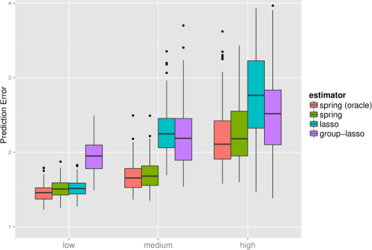
Figure 2: Illustration of the influence of correlations between outcomes. Scenarios $\left\{\text{low},\text{med},\text{high}\right\}$ map to $\tau\in\left\{.1,.5,.9\right\}$ in the Toeplitz-shaped covariance matrix $\mathbf{R}$.

4.2 Structure integration and robustness

The second simulation study is designed to measure the impact of introducing an informative prior along the predictors via $\mathbf{L}$. To remove any effect induced by the covariance between the outputs, we set $q=1$. In this case the criterion is written as in Expression (8): $\mathbf{R}$ boils down to a scalar $\sigma^{2}$ and $\mathbf{B},\boldsymbol{\Omega}_{\mathbf{x}\mathbf{y}}$ turn to two $p$-size vectors sharing the same sparsity pattern such that $\boldsymbol{\beta}=-\boldsymbol{\omega}\sigma^{2}$. In this situation, SPRING is close to [32]’s structured Elastic-Net, except that we hope for a better estimation of the coefficients thanks to the estimation of $\sigma$. For comparison, we thus draw inspiration from the simulation settings originally used to illustrate the structured Elastic-Net: we set $\boldsymbol{\omega}=(\omega_{j})_{j=1}^{p},$ with $p=100$, so that we observe a sparse vector with two smooth bumps, one positive and the other one negative:

$$\omega_{j}=\begin{cases}-((30-j)^{2}-100)/200&j=21,\dots 39,\\ \ \ \ ((70-j)^{2}-100)/200&j=61,\dots 80,\\ 0&\text{otherwise}.\end{cases}$$

A natural choice for $\mathbf{L}$ is to rely on the first forward difference operator as in the fused-Lasso ([37]), or its smooth counterpart ([11]). We thus set $\mathbf{L}=\mathbf{D}^{T}\mathbf{D}$ with

$$\mathbf{D}_{ij}=\begin{cases}1&\text{if }i=j,\\ -1&\text{if }j=i+1\\ 0&\text{otherwise}\\ \end{cases},\quad\begin{array}[]{c}i=1,\dots,p-1,\\ j=1,\dots,p.\end{array}$$ (10)

Hence, $\mathbf{L}$ is the combinatorial Laplacian of a chain graph between the successive predictors.

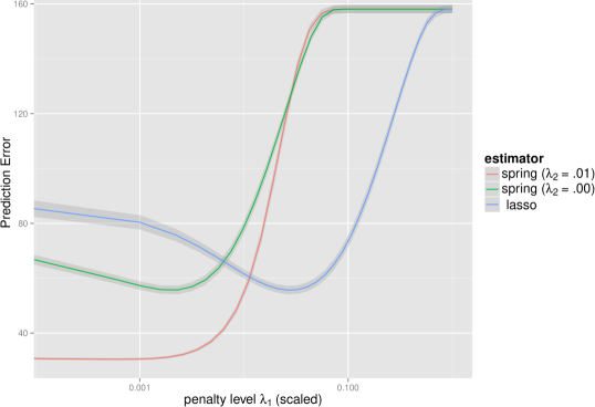
Figure 3: Illustrating gain brought by structure information toward predictive performance

Figure 3 shows the typical gain brought by prior structure knowledge. We generate $100$ learning samples of size $n=100$ with $\sigma^{2}=5$ and represent the averaged PE curves as a function of $\lambda_{1}$ for the LASSO and for two versions of SPRING, with ($\lambda_{2}=.01$) and without ($\lambda_{2}=0$) informative prior. Incorporating relevant structural information leads to a dramatic improvement. As expected, univariate SPRING with no prior performs like the LASSO, in the sense that they share the same minimal PE.

Now, the question is: what if we introduce a wrong prior, i.e. a matrix $\mathbf{L}$ completely disconnected from the true structure of the coefficients? To answer this question, we use the same settings as above and randomly swap the entries in $\boldsymbol{\omega}$, using exactly the same $\mathbf{x}_{i}$ to generate the $\mathbf{y}_{i}$. We then apply SPRING using respectively a non informative prior equal to the identity matrix (thus mimicking the Elastic-Net) and a ’wrong’ prior $\mathbf{L}$ whose rows and columns remain unswapped. We also try the LASSO, the Elastic-Net and the structured Elastic-Net. All methods are tuned with 5-fold cross-validation on the learning set. Table I presents the results averaged over 100 runs both in terms of PE (using a size-1000 test set) and MSE.

Method	Scenario	MSE	PE
LASSO	–	.336 (.096)	58.6 (10.2)
E-Net ($\mathbf{L}=\mathbf{I}$)	–	.340 (.095)	59 (10.3)
SPRING ($\mathbf{L}=\mathbf{I}$)	–	.358 (.094)	60.7 (10)
S. E-net	unswapped	.163 (.036)	41.3 ( 4.08)
($\mathbf{L}=\mathbf{D}^{T}\mathbf{D}$)	swapped	.352 (.107)	60.3 (11.42)
SPRING	unswapped	.062 (.022)	31.4 ( 2.99)
($\mathbf{L}=\mathbf{D}^{T}\mathbf{D}$)	swapped	.378 (.123)	62.9 (13.15)

Table I: Structure integration: performance and robustness. Swapped and unswapped results are the same for LASSO, Elastic-Net and SPRING for $\mathbf{L}=\mathbf{I}$.

As expected, the methods that do not integrate any structural information (LASSO, Elastic-Net and SPRING with $\mathbf{L}=\mathbf{I}$) are not affected by the permutation, and we avoid these redundancies in Table I to save space. Overall, they share similar performance both in terms of PE and MSE. When the prior structure is relevant, SPRING, and to a lesser extent the structured Elastic-Net, clearly outperform the other competitors. Surprisingly, this is particularly true in terms of MSE, where SPRING also dominates the structured Elastic-Net that works with the same information. This means that the estimation of the variance also helped in the inference process. Finally, these results essentially support the robustness of the structured methods which are not much altered when using a wrong prior specification.

5 Application Studies

In this section the flexibility of our proposal is illustrated by investigating three multivariate data problems from various contexts, namely spectroscopy, genetics and genomics, where we insist on the construction of the structuring matrix $\mathbf{L}$.

5.1 Near-Infrared Spectroscopy of Cookie Dough Pieces

Context

In Near-Infrared (NIR) spectroscopy, one aims to predict one or several quantitative variables from the NIR spectrum of a given sample. Each sampled spectrum is a curve that represents the level of reflectance along the NIR region, that is, wavelengths from 800 to 2500 nanometers (nm). The quantitative variables are typically related to the chemical composition of the sample. The problem is then to select the most predictive region of the spectrum, i.e. some peaks that show good capabilities for predicting the response variable(s). This is known as a “calibration problem” in Statistics. NIR technique is used in fields as diverse as agronomy, astronomy or pharmacology. In such experiments, it is likely to encounter very strong correlations and structure along the predictors. In this perspective, [9] proposes to apply the Elastic-Net which is known to select simultaneously groups of correlated predictors. However it is not adapted to the prediction of several responses simultaneously. In [2], an interesting wavelet regression model with Bayesian inference is introduced that enters the multivariate regression model, as does our proposal.

Description of the dataset

We consider the cookie dough data from [26]. The data with the corresponding test and training sets are available in the fds R package. After data pretreatments as in [2], we have $n=39$ dough pieces in the training set: each sample consists in an NIR spectrum with $p=256$ points measured from 1380 to 2400 nm (spaced by 4 nm), and in four quantitative variables that describe the percentages of fat, sugar flour and water of in the piece of dough.

Structure specification

We would like to account for the neighborhood structure between the predictors which is obvious in the context of NIR spectroscopy: since spectra are continuous curves, a smooth neighborhood prior will encourage predictors to be selected by “wave”, which seems more satisfactory than isolated peaks. Thus, we naturally define $\mathbf{L}$ by means of the first forward difference operator (10). We also tested higher orders of the operator to induce a stronger smoothing effect, but they do not lead to dramatic changes in terms of PE and we omit them. Order $k$ is simply obtained by powering the first order matrix. Such techniques have been studied in a structured $\ell_{1}$-penalty framework in [15, 38] and is known as trend filtering. Our approach however is different, though: it enters a multivariate framework and is based on a smooth $\ell_{2}$-penalty coupled with the $\ell_{1}$-penalty for selection.

Results

The predictive performance of a series of regression techniques is compared in Table II, evaluated on the same test set.

Method	fat	sucrose	flour	water
Stepwise MLR	.044	1.188	.722	.221
Decision theory	.076	.566	.265	.176
PLS	.151	.583	.375	.105
PCR	.160	.614	.388	.106
Wavelet Regression	.058	.819	.457	.080
LASSO	.044	.853	.370	.088
group-LASSO	.127	.918	.467	.102
MRCE	.151	.821	.321	.081
Structured E-net	.044	.596	.363	.082
SPRING (CV)	.065	.397	.237	.083
SPRING (BIC)	.048	.389	.243	.066

Table II: Prediction error for the cookie dough data.

The first four rows (namely stepwise multivariate regression, Bayesian decision theory approach, Partial Least Square and Principal Component Regression) correspond to calibration methods originally presented in [2]; row five (Bayesian Wavelet Regression) is the original proposal from [2]; the remainder of the table is due to our own analysis. We observe that, on this example, SPRING achieves extremely competitive results. The BIC performs notably well as a model selection criterion.

LASSO	group-LASSO	Structured Elastic-Net	MRCE
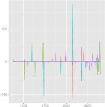
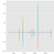
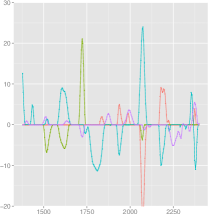
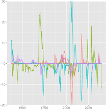
Wavelength range (nanometer)

Figure 4: Parameters estimated by the penalized regression methods for the cookie data

Figure 4 shows the regression coefficients adjusted with the penalized regression techniques: apart from LASSO which selects very isolated (and unstable) wavelengths, non-zero regression coefficients have quite a wide spread, and therefore hard to interpret. As expected, the multitask group-Lasso activates the same predictors across the responses, which is not a good idea when looking at the predictive performance in Table II. On the other hand, in Figure 5, the direct effects selected by SPRING with BIC define predictive regions specific to each response which are well suited for interpretability purposes.

	$\hat{\mathbf{B}}$ (indirect effects)	$-\hat{\boldsymbol{\Omega}}_{\mathbf{x}\mathbf{y}}$ (direct effects)	$\hat{\mathbf{R}}$
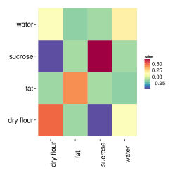
	wavelength range (nanometer)

Figure 5: Parameters estimated by our proposal for the cookie dough data (better seen in color). Since $\hat{\mathbf{B}}$ and $\hat{\boldsymbol{\Omega}}_{\mathbf{x}\mathbf{y}}$ are opposite in sign in our model, we represent $-\hat{\boldsymbol{\Omega}}_{\mathbf{x}\mathbf{y}}$ to ease the comparison between direct and indirect effects.

Parameters fitted by our approach with BIC are represented on Figure 5 with, from left to right, the estimators of the regression coefficients $\mathbf{B}$, of the direct effects $\boldsymbol{\Omega}_{\mathbf{x}\mathbf{y}}$ and of the residual covariance $\mathbf{R}$. The regression coefficients show no sparsity pattern but a strong spatial structure along the spectrum, characterized by waves induced by a smooth first order difference prior. Concerning a potential structure between the outputs, we identify interesting regions where a strong correlation between the responses induces correlations between the regression coefficients. Consider for instance positions of the wavelength between 1750 and 2000 nm: the regression parameters related to “dry-flour” are clearly anti-correlated with those related to “sucrose”. Still, we cannot distinguish in $\hat{\mathbf{B}}$ for a direct effect of this region on either the flour or sucrose composition. Such a distinction is achieved on the middle panel where direct effects $\hat{\boldsymbol{\Omega}}_{\mathbf{x}\mathbf{y}}$ selected are plotted: it defines sparse predictive regions specific to each response which are well suited for interpretability purposes; in fact, it is now obvious that region 1750 to 2000 is rather linked to the sucrose.

5.2 Multi-trait Genomic Selection in Brassica napus

Context

Genomic selection is aimed at predicting one or several phenotypes based on the information of genetic markers. To this end, regularization methods such as ridge or Lasso regression or their Bayesian counterparts have been proposed ([4]). Still, in most studies only single trait genomic selection is performed, neglecting correlations between phenotypes. Moreover, little attention has been devoted to the development of regularization methods including prior genetic knowledge.

Description of the dataset

We consider the Brassica napus dataset described in [6] and [16]. Data consists in $n=103$ double-haploid lines derived from 2 parent cultivars, ‘Stellar’ and ‘Major’, on which $p=300$ genetic markers and $q=8$ traits (responses) were recorded. Each marker is a 0/1 covariate with $x_{i}^{j}=0$ if line $i$ has the ’Stellar’ allele at marker $j$, and $x_{i}^{j}=1$ otherwise. Traits included are percent winter survival for 1992, 1993, 1994, 1997 and 1999 (surv92, surv93, surv94, surv97, surv99, respectively), and days to flowering after no vernalization (flower0), 4 weeks vernalization (flower4) or 8 weeks vernalization (flower8).

Structure specification

In a biparental line population, correlation between 2 markers depends on their genetic distance defined in terms of recombination fraction. As a consequence, one expects adjacent markers on the sequence to be correlated, yielding similar direct relationships with the phenotypic traits. Noting $d_{12}$ the genetic distance between markers $M_{1}$ and $M_{2}$, one has $\text{cor}(M_{1},M_{2})=\rho^{d_{12}}$, where $\rho=.98$. The covariance matrix $\mathbf{L}^{-1}$ can hence be defined as $\mathbf{L}_{ij}^{-1}=\rho^{d_{ij}}$. Moreover, assuming recombination events are independent between $M_{1}$ and $M_{2}$ on the one hand, and $M_{2}$ and $M_{3}$ on the other hand, one has $d_{13}=d_{12}+d_{23}$ and matrix $\mathbf{L}^{-1}$ exhibits an inhomogeneous AR(1) profile. As a consequence, $\mathbf{L}$ is tridiagonal with general elements

$$w_{i,i} = \frac{1-\rho^{2d_{i-1,i}+2d_{i,i+1}}}{(1-\rho^{2d_{i-1,i}})(1-\rho^{2d_{i,i+1}})},$$

$$w_{i,i+1} = \frac{-\rho^{d_{i,i+1}}}{1-\rho^{2d_{i,i+1}}}$$

and $w_{i,j}=0$ if $|i-j|>1$. For the first (resp. last) marker, the distance $d_{i-1,i}$ (resp. $d_{i,i+1}$) is infinite.

Results

To compare SPRING and its competitors in terms of predictive performance, PE is estimated by randomly splitting the $103$ samples into training and test sets with sizes 93 and 10. Before adjusting the models, we first scale the outcomes on the training and test sets to facilitate interpretability. Five-fold cross-validation is used on the training set to choose the tuning parameters. Two hundred random samplings of the test and training sets were conducted to estimate the PE given in Table III.

Method	surv92	surv93	surv94	surv97	surv99
LASSO	.730 (.011)	.977 (.009)	.943 (.010)	.947 (.009)	.916 (.010)
S. Enet	.697 (.011)	.987 (.009)	.941 (.011)	.945 (.009)	.911 (.010)
MRCE	.759 (.010)	.919 (.003)	917 (.006)	.924 (.004)	.926 (.006)
SPRING	.724 (.010)	.948 (.008)	.848 (.010)	.940 (.006)	.907 (.009)

Method	flower0	flower4	flower8
LASSO	.609 (.011)	.501 (.011)	.744 (.011)
S. Enet	.577 (.011)	.478 (.010)	.727 (.012)
MRCE	.591 (.011)	.479 (.011)	.736 (.011)
SPRING	.489 (.010)	.419 (.009)	.616 (.012)

Table III: Estimated prediction error for the Brassica napus data (standard error in parentheses)

All methods provide similar results although SPRING provides the smallest error for half of the traits. A picture of the between-response covariance matrix estimated with SPRING is given in Figure 6. It reflects the correlation between the traits, which are either explained by an unexplored part of the genotype, by the environment or by some interaction between the two. The residuals of the flowering times exhibit strong correlations, whereas correlations between the survival rates are weak. It also shows that the survival traits have a larger residual variability than do the flowering traits, suggesting a higher sensitivity to environmental conditions.

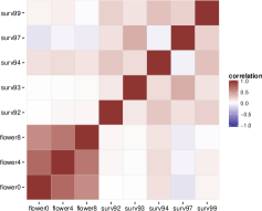
Figure 6: Brassica study: residual covariance estimation

We then turn to the effects of each marker on the different traits. The left panels of Figure 7 give both the regression coefficients (top) and the direct effects (bottom). The gray zones correspond to chromosomes 2, 8 and 10, respectively. The exact location of the markers within these chromosomes is displayed in the right panels, where the size of the dots reflects the absolute value of the regression coefficients (top) and of the direct effects (bottom).

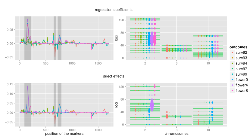
Figure 7: Brassica Study: direct and indirect genetic effects of the markers on the traits estimated by SPRING (better seen in color).

The interest of considering direct effects rather than regression coefficients appears clearly here, if one looks for example at chromosome 2. Three large overlapping regions are observed in the coefficient plot, for each flowering trait. A straightforward interpretation would suggest that the corresponding region controls the general flowering process. The direct effect plot allows one to go deeper and shows that these three responses are actually controlled by three separate sub-regions within this chromosome. The confusion in the coefficient plot only results from the strong correlations observed among the three flowering traits.

5.3 Selecting regulatory motifs from multiple microarrays

5.3.1 Context

In genomics, the expression of genes is initiated by transcription factors that bind to the DNA upstream from the coding regions, called regulatory regions. This binding occurs when a given factor recognizes a certain (small) sequence called a regulatory motif. Genes hosting the same regulatory motif will be jointly expressed under certain conditions. As the binding relies on chemical affinity, some degeneracy can be tolerated in the motif definition, and motifs similar but for small variations may share the same functional properties (see, e.g. [17]).

We are interested in the detection of such regulatory motifs, the presence of which controls the gene expression profile. To this aim we try to establish a relationship between the expression level of all genes across a series of conditions with the content of their respective regulatory regions in terms of motifs. In this context, we expect $i)$ the set of influential motifs to be small for each condition, $ii)$ the influential motifs for a given condition to be degenerate versions of each other, and $iii)$ the expression under similar conditions to be controlled by the same motifs.

Description of the dataset

In [8], a series of microarray experiments are conducted on yeast cells (Saccharomyces cerevisae). Among these assays, we consider 12 time-course experiments profiling $n=5883$ genes under various environmental changes as listed in Table IV. These expression sets form 12 potential response matrices $\mathbf{Y}$, the column number of which corresponds to the number of time points.

Experiment	# time point	# motifs selected
		$k=7$	$k=8$	$k=9$
Heat shock	8	30	68	43
Shift from 37°to 25 °C	5	3	11	33
Mild Heat shock	4	24	13	23
Response to $\text{H}_{2}\text{O}_{2}$	10	15	10	21
Menadione Exposure	9	16	1	7
DDT exposure 1	8	15	10	30
DDT exposure 2	7	11	33	21
Diamide treatment	8	45	25	35
Hyperosmotic shock	7	36	24	15
Hypo-osmotic shock	5	20	8	29
Amino-acid starvation	5	47	30	39
Diauxic Shift	7	16	14	20
total number of unique motifs inferred		87	82	72

Table IV: Time-course data from [8] considered for regulatory motif discovery

Concerning the predictors, we consider the set of all motifs with length $k$ formed with the four nucleotides, that is $\mathcal{M}_{k}=\left\{A,C,G,T\right\}^{k}$. There are $p=|\mathcal{M}_{k}|=4^{k}$ such motifs. Unless otherwise stated, the motifs in $\mathcal{M}$ are lined up in lexicographical order e.g., when $k=2$, $AA,AC,AG,AT,CA,CC,\dots$ and so on. Then, the $n\times p$ matrix of predictors $\mathbf{X}$ is filled such that $X_{ij}$ equals the occurrence count of motif $j$ in the regulatory region of gene $i$.

Structure specification

As we expect influential motifs for a given condition to be degenerate versions of each other, we first measure the similarity between any two motifs from $\mathcal{M}_{k}$ with the Hamming defined as

$$\forall a,b\in\mathcal{M}_{k},\quad\mathrm{dist}(a,b)=\text{card}\{i:a_{i}\neq b_{i}\}.$$

For a fixed value of interest $0\leq\ell\leq k$, we further define the $\ell$-distance matrix $\mathbf{D}^{k,\ell}=(d^{k,\ell}_{ab})_{a,b\in\mathcal{M}_{k}}$ as

$$\forall a,b\in\mathcal{M}_{k},\quad d^{k,\ell}_{ab}=\left\{\begin{array}[]{ll}1&\text{if $\mathrm{dist}(a,b)\leq\ell$}\\ 0&\text{otherwise.}\\ \end{array}\right.$$

$\mathbf{D}^{k,\ell}$ can be viewed as the adjacency matrix of a graph where the nodes are the motifs and where an edge is present between 2 nodes when the 2 motifs are at a Hamming distance less or equal to $\ell$. We finally use the Laplacian of this graph as a structuring matrix $\mathbf{L}^{k,\ell}=(\ell^{k,\ell}_{ab})_{a,b\in\mathcal{M}_{k}}$, that is

$$\ell^{k,\ell}_{ab}=\begin{cases}\sum_{c\in\mathcal{M}_{k}}d^{k,\ell}_{ac}&\text{if }a=b,\\ -1&\text{if }d^{k,\ell}_{ab}=1,\\ 0&\text{otherwise}.\end{cases}$$ (11)

Note that we came across a similar proposal by [20] in the context of sparse, structured PLS. The derivation, however, is different, and the objective of this method is not the selection of motifs but of families of motifs via the compression performed by the PLS.

Results

We apply our methodology for candidate motifs from $\mathcal{M}_{7},\mathcal{M}_{8}$ and $\mathcal{M}_{9}$, which results in three lists of putative motifs having a direct effect on gene expression. Due to the very large number of potential predictors that comes with a sparser matrix $\mathbf{X}$ when $k$ increases, we first perform a screening step that keeps the $5,000$ motifs with the highest marginal correlations with $\mathbf{Y}$. Second, SPRING is applied to each of the twelve time-course experiments described in Table IV. The selection of $(\lambda_{1},\lambda_{2})$ is performed on a grid using the BIC (3.2). At the end of the day, the three lists corresponding to $k=7,8,9$ include respectively 87, 82 and 72 motifs, for which at least one coefficient in the associated row $\widehat{\boldsymbol{\Omega}}_{\mathbf{x}\mathbf{y}}(j,\cdot)$ was found non-null for some of the twelve experiments, as detailed in Table IV.

To assess the relevance of the selected motifs, we compared them with the MotifDB patterns available in Bioconductor ([31]), where known transcription factor binding sites are recorded. There are 453 such reference motifs with size varying from 5 to 23 nucleotides. Consider the case of $k=7$ for instance: among the 87 SPRING motifs, 62 match one MotifDB pattern each and 25 are clustered into 11 MotifDB patterns as depicted in Table 5.3.

CTAAGCCAC   TAGCCCC   GCGCCCC	GCATGTGAA CCATATG   TTGTGAG	CATGTAATT   TGTAAAT   TGTATAT	TGAAACA TTAGACC TAAAAAG
TGATCGGCGCCGCACGACGA            GTATAAC       GCGCCGT	TGCTGGTT  GCTGGTT  GCTGGTG	GATCGTATGATA  ATCATAT  TTGGTAT	ACGCGAAAA  AACGAAA   ACGAAAA
CCATACATCAC  CATAGAC     ATATCAC	ATTGACCTGGTC  TCGACTT   CGACTTG      CCAGCTT	GACTAGATATATATATTCGAT           ATATATT        CATATAT           ATATATG         ATATATA

Table V: Comparison of SPRING-selected motifs with MotifDB patterns. Each cell corresponds to a MotifDB pattern (top) compared to a set of aligned SPRING motifs with size 7 (down).

As seen in this table, the clusters of motifs selected by SPRING correspond to sets of variants of the same pattern. These clusters consist of motifs that are close according to the similarity encoded in the structure matrix $\mathbf{L}$. In this example, the ability of SPRING to use domain-specific definitions of the structure between the predictors oriented the regression problem to account for motif degeneracy and helped in selecting motifs that are consistent known binding sites.

Appendix A Proofs

Most of the proofs rely on basic algebra and properties of the trace and the $\mathrm{vec}$ operators (see e.g. [10]), in particular

$$\mathrm{tr}(\mathbf{A}^{T}\mathbf{B}\mathbf{C}\mathbf{D}^{T})=\mathrm{vec}(\mathbf{A})^{T}(\mathbf{D}\otimes\mathbf{B})\mathrm{vec}(\mathbf{C}),$$

$$\mathrm{vec}(\mathbf{A}\mathbf{B}\mathbf{C})=(\mathbf{C}^{T}\otimes\mathbf{A})\mathrm{vec}(\mathbf{B}),$$

$$(\mathbf{A}\otimes\mathbf{B})(\mathbf{C}\otimes\mathbf{D})=(\mathbf{A}\mathbf{C})\otimes(\mathbf{C}\mathbf{D}).$$

A.1 Derivation of Proposition 1

Concerning the two regularization terms in (7), we have $\|\boldsymbol{\Omega}_{\mathbf{x}\mathbf{y}}\|_{1}=\|\boldsymbol{\omega}\|_{1}$ since the $\ell_{1}$-norm applies element-wise here and

$$\mathrm{tr}(\boldsymbol{\Omega}_{\mathbf{y}\mathbf{x}}\mathbf{L}\boldsymbol{\Omega}_{\mathbf{x}\mathbf{y}}\boldsymbol{\Omega}_{\mathbf{y}\mathbf{y}}^{-1})=\boldsymbol{\omega}^{T}(\boldsymbol{\Omega}_{\mathbf{y}\mathbf{y}}^{-1}\otimes\mathbf{L})\boldsymbol{\omega}.$$

As for the log-likelihood (5), we work on the trace term:

$$\mathrm{tr}\left(\left(\mathbf{Y}+\mathbf{X}\boldsymbol{\Omega}_{\mathbf{x}\mathbf{y}}\boldsymbol{\Omega}_{\mathbf{y}\mathbf{y}}^{-1}\right)^{T}\left(\mathbf{Y}+\mathbf{X}\boldsymbol{\Omega}_{\mathbf{x}\mathbf{y}}\boldsymbol{\Omega}_{\mathbf{y}\mathbf{y}}^{-1}\right)\boldsymbol{\Omega}_{\mathbf{y}\mathbf{y}}\right)=\\ \mathrm{vec}\left(\mathbf{Y}+\mathbf{X}\boldsymbol{\Omega}_{\mathbf{x}\mathbf{y}}\boldsymbol{\Omega}_{\mathbf{y}\mathbf{y}}^{-1}\right)^{T}\left(\boldsymbol{\Omega}_{\mathbf{y}\mathbf{y}}\otimes\mathbf{I}_{n}\right)\mathrm{vec}\left(\mathbf{Y}+\mathbf{X}\boldsymbol{\Omega}_{\mathbf{x}\mathbf{y}}\boldsymbol{\Omega}_{\mathbf{y}\mathbf{y}}^{-1}\right)\\ =\left\|\left(\boldsymbol{\Omega}_{\mathbf{y}\mathbf{y}}\otimes\mathbf{I}_{n}\right)^{1/2}\left(\mathrm{vec}(\mathbf{Y})+\left(\boldsymbol{\Omega}_{\mathbf{y}\mathbf{y}}^{-1}\otimes\mathbf{X}\right)\mathrm{vec}(\boldsymbol{\Omega}_{\mathbf{x}\mathbf{y}})\right)\right\|_{2}^{2}\\ =\left\|\mathrm{vec}(\mathbf{Y}\boldsymbol{\Omega}_{\mathbf{y}\mathbf{y}}^{1/2})+\left(\boldsymbol{\Omega}_{\mathbf{y}\mathbf{y}}^{-1/2}\otimes\mathbf{X}\right)\boldsymbol{\omega}\right\|_{2}^{2}.$$

The rest of the proof is straightforward.

A.2 Convexity lemma

Lemma 1.

The function

$$-\frac{1}{n}\log L(\boldsymbol{\Omega}_{\mathbf{x}\mathbf{y}},\boldsymbol{\Omega}_{\mathbf{y}\mathbf{y}})+\frac{\lambda_{2}}{2}\mathrm{tr}\left(\boldsymbol{\Omega}_{\mathbf{y}\mathbf{x}}\mathbf{L}\boldsymbol{\Omega}_{\mathbf{x}\mathbf{y}}\boldsymbol{\Omega}_{\mathbf{y}\mathbf{y}}^{-1}\right)$$

is jointly convex in $(\boldsymbol{\Omega}_{\mathbf{x}\mathbf{y}},\boldsymbol{\Omega}_{\mathbf{y}\mathbf{y}})$ and admits at least one global minimum which is unique when $n\geq q$ and $(\lambda_{2}\mathbf{L}+\mathbf{S}_{\mathbf{x}\mathbf{x}})$ is positive definite.

The convexity of $-\frac{1}{n}\log L(\boldsymbol{\Omega}_{\mathbf{x}\mathbf{y}},\boldsymbol{\Omega}_{\mathbf{y}\mathbf{y}})$ is proved in [43] (Proposition 1). Similar arguments can be straightforwardly applied in the case at hand. Existence of the global minimum is related to strict convexity in both $\boldsymbol{\Omega}_{\mathbf{x}\mathbf{y}}$ and $\boldsymbol{\Omega}_{\mathbf{y}\mathbf{y}}$, where direct differentiation leads to the corresponding conditions.

A.3 Proof of Theorem 1

The convexity of criterion $J(\boldsymbol{\Omega}_{\mathbf{x}\mathbf{y}},\boldsymbol{\Omega}_{\mathbf{y}\mathbf{y}})$ in $(\boldsymbol{\Omega}_{\mathbf{x}\mathbf{y}},\boldsymbol{\Omega}_{\mathbf{y}\mathbf{y}})$ is straightforward thanks to Lemma 1 and considering the fact that $\|\boldsymbol{\Omega}_{\mathbf{x}\mathbf{y}}\|_{1}$ is also convex. One can then apply the results developed in [41, 40] on the convergence of block coordinate descent for the minimization of nonsmooth separable function. Since (7) is clearly separable in $(\boldsymbol{\Omega}_{\mathbf{x}\mathbf{y}},\boldsymbol{\Omega}_{\mathbf{y}\mathbf{y}})$ for the nonsmooth part induced by the $\ell_{1}$-norm, the alternating scheme is guaranteed to converge to the unique global minimum under the assumption of Lemma 1. It remains to show that the two convex optimization subproblems (9a) and (9b) can be (efficiently) solved in practice.

Firstly, (9b) can be recast as an Elastic-Net problem, which in turn can be recast as a LASSO problem (see, e.g. [44, 32]). This is straightforward thanks to Proposition 1: when $\hat{\boldsymbol{\Omega}}_{\mathbf{y}\mathbf{y}}$ is fixed, solution to (9b) can be obtained via

$$\hat{\boldsymbol{\omega}}\left(=\mathrm{vec}(\hat{\boldsymbol{\Omega}}_{\mathbf{x}\mathbf{y}})\right)\\ =\mathop{\mathrm{arg\ min}}_{\boldsymbol{\omega}\in\mathbb{R}^{pq}}\frac{1}{2}\|\mathbf{A}\boldsymbol{\omega}-\mathbf{b}\|_{2}^{2}+\frac{\lambda_{2}}{2}\boldsymbol{\omega}^{T}\tilde{\mathbf{L}}\boldsymbol{\omega}+\lambda_{1}\|\boldsymbol{\omega}\|_{1},$$ (12)

where $\mathbf{A},\mathbf{b}$ and $\tilde{\mathbf{L}}$ are defined by

$$\mathbf{A}=\left(\hat{\boldsymbol{\Omega}}_{\mathbf{y}\mathbf{y}}^{-1/2}\otimes\mathbf{X}/\sqrt{n}\right),\\ \mathbf{b}=-\mathrm{vec}\left(\mathbf{Y}\hat{\boldsymbol{\Omega}}_{\mathbf{y}\mathbf{y}}^{1/2}\right)/\sqrt{n}\text{ and }\tilde{\mathbf{L}}=\hat{\boldsymbol{\Omega}}_{\mathbf{y}\mathbf{y}}^{-1}\otimes\mathbf{L}.$$

Secondly, we can solve analytically (9a) with simple matrix algebra. By differentiation of the objective (7) over $\boldsymbol{\Omega}_{\mathbf{y}\mathbf{y}}^{-1}$ we obtain the quadratic form

$$\boldsymbol{\Omega}_{\mathbf{y}\mathbf{y}}\mathbf{S}_{\mathbf{y}\mathbf{y}}\boldsymbol{\Omega}_{\mathbf{y}\mathbf{y}}-\boldsymbol{\Omega}_{\mathbf{y}\mathbf{y}}=\boldsymbol{\Omega}_{\mathbf{y}\mathbf{x}}(\lambda_{2}\mathbf{L}+\mathbf{S}_{\mathbf{x}\mathbf{x}})\boldsymbol{\Omega}_{\mathbf{x}\mathbf{y}}.$$

After right multiplying both sides by $\mathbf{S}_{\mathbf{y}\mathbf{y}}$, it becomes obvious that $\boldsymbol{\Omega}_{\mathbf{y}\mathbf{y}}\mathbf{S}_{\mathbf{y}\mathbf{y}}$ and $\boldsymbol{\Omega}_{\mathbf{y}\mathbf{x}}(\lambda_{2}\mathbf{L}+\mathbf{S}_{\mathbf{x}\mathbf{x}})\boldsymbol{\Omega}_{\mathbf{x}\mathbf{y}}\mathbf{S}_{\mathbf{y}\mathbf{y}}$ commute and thus share the same eigenvectors $\mathbf{U}$. Besides, it induces the relationship $\eta_{j}^{2}-\eta_{j}=\zeta_{j}$ between their respective eigenvalues $\eta_{j}$ and $\zeta_{j}$, and we are looking for the positive solution of $\eta_{j}$. To do so, first note that we may assume that $\boldsymbol{\Omega}_{\mathbf{y}\mathbf{x}}(\lambda_{2}\mathbf{L}+\mathbf{S}_{\mathbf{x}\mathbf{x}})\boldsymbol{\Omega}_{\mathbf{x}\mathbf{y}}$ and $\mathbf{S}_{\mathbf{y}\mathbf{y}}$ are positive definite, when $\boldsymbol{\Omega}_{\mathbf{x}\mathbf{y}}\neq\mathbf{0}$ and $n\geq q$; and second, recall that if a matrix is the product of two positive definite matrices then its eigenvalues are positive. Hence, $\zeta_{j}>0$ and the positive solution of $\eta_{j}$ is $\eta_{j}=(1+\sqrt{1+4\zeta_{j}})/2$. We thus obtain

$$\hat{\boldsymbol{\Omega}}_{\mathbf{y}\mathbf{y}}=\mathbf{U}\mathrm{diag}(\boldsymbol{\eta})\mathbf{U}^{-1}\mathbf{S}_{\mathbf{y}\mathbf{y}}^{-1}.$$ (13)

Direct inversion yields

$$\hat{\boldsymbol{\Omega}}_{\mathbf{y}\mathbf{y}}=\mathbf{U}\mathrm{diag}(\boldsymbol{\eta}/\boldsymbol{\zeta})\mathbf{U}^{-1}\hat{\boldsymbol{\Omega}}_{\mathbf{y}\mathbf{x}}(\lambda_{2}\mathbf{L}+\mathbf{S}_{\mathbf{x}\mathbf{x}})\hat{\boldsymbol{\Omega}}_{\mathbf{x}\mathbf{y}}(=\hat{\mathbf{R}}^{-1}),$$

To get an expression for $\hat{\boldsymbol{\Omega}}_{\mathbf{y}\mathbf{y}}$ which does not require additional matrix inversion, just note that

$$\mathbf{S}_{\mathbf{y}\mathbf{y}}^{-1}=\left(\boldsymbol{\Omega}_{\mathbf{y}\mathbf{x}}\hat{{\boldsymbol{\Sigma}}}_{\mathbf{x}\mathbf{x}}^{\lambda_{2}}\boldsymbol{\Omega}_{\mathbf{x}\mathbf{y}}\mathbf{S}_{\mathbf{y}\mathbf{y}}\right)^{-1}\boldsymbol{\Omega}_{\mathbf{y}\mathbf{x}}\hat{{\boldsymbol{\Sigma}}}_{\mathbf{x}\mathbf{x}}^{\lambda_{2}}\boldsymbol{\Omega}_{\mathbf{x}\mathbf{y}}\\ =\mathbf{U}\mathrm{diag}(\boldsymbol{\zeta}^{-1})\mathbf{U}^{-1}\boldsymbol{\Omega}_{\mathbf{y}\mathbf{x}}\hat{{\boldsymbol{\Sigma}}}_{\mathbf{x}\mathbf{x}}^{\lambda_{2}}\boldsymbol{\Omega}_{\mathbf{x}\mathbf{y}}$$

where $\hat{{\boldsymbol{\Sigma}}}_{\mathbf{x}\mathbf{x}}^{\lambda_{2}}=(\lambda_{2}\mathbf{L}+\mathbf{S}_{\mathbf{x}\mathbf{x}})$. Combined with(13), this last equality leads to

$$\hat{\boldsymbol{\Omega}}_{\mathbf{y}\mathbf{y}}^{-1}=\mathbf{S}_{\mathbf{y}\mathbf{y}}\mathbf{U}\mathrm{diag}(\boldsymbol{\eta}^{-1})\mathbf{U}^{-1}(=\hat{\mathbf{R}}).$$

Finally, in the particular case where $\hat{\boldsymbol{\Omega}}_{\mathbf{x}\mathbf{y}}=\mathbf{0}$, $\hat{\boldsymbol{\Omega}}_{\mathbf{y}\mathbf{y}}=\mathbf{S}_{\mathbf{y}\mathbf{y}}^{-1}$.

A.4 Derivation of Proposition 2

To apply the results developed in [39] that rely on the well-known Stein’s Lemma ([35]), we basically need to recast our problem as a classical LASSO applied on a Gaussian linear regression model such that the response vector follows a normal distribution of the form $\mathcal{N}({\boldsymbol{\mu}},\sigma\mathbf{I})$. This is straightforward by means of Proposition 1: in the same way as we derive expression (12), we can go a little further and reach the following LASSO formulation

$$\mathop{\mathrm{arg\ min}}_{\boldsymbol{\omega}\in\mathbb{R}^{pq}}\frac{1}{2}\left\|\begin{pmatrix}\mathbf{A}\\ \sqrt{\lambda_{2}}\tilde{\mathbf{L}}^{1/2}\end{pmatrix}\boldsymbol{\omega}-\begin{pmatrix}\mathbf{b}\\ \mathbf{0}\end{pmatrix}\right\|_{2}^{2}+\lambda_{1}\|\boldsymbol{\omega}\|_{1},$$ (14)

with $\mathbf{A},\mathbf{b}$ and $\tilde{\mathbf{L}}$ defined as in (12). From model (4), it is not difficult to see that $\mathbf{b}$ corresponds to an uncorrelated vector form of $\mathbf{Y}$ so as

$$\begin{pmatrix}\mathbf{b}\\ \mathbf{0}\end{pmatrix}=\begin{pmatrix}-\mathrm{vec}(\mathbf{Y}\boldsymbol{\Omega}_{\mathbf{y}\mathbf{y}}^{1/2})\\ \mathbf{0}\end{pmatrix}\sim\mathcal{N}({\boldsymbol{\mu}},\mathbf{I}_{nq}).$$

The explicit form of ${\boldsymbol{\mu}}$ is of no interest here. The point is essentially to underline that the response vector is uncorrelated in (14), which allows us to apply Theorem 2 of [39] and results therein, notably for the Elastic-Net. By these means, an unbiased estimator of the degrees of freedom in (14) can be written as a function of the active set $\mathcal{A}$ in $\hat{\boldsymbol{\omega}}^{\lambda_{1},\lambda_{2}}$:

$$\hat{\mathrm{df}}_{\lambda_{1},\lambda_{2}}=\mathrm{tr}\left(\mathbf{A}_{\mathcal{A}}\left((\mathbf{A}^{T}\mathbf{A}+\lambda_{2}\tilde{\mathbf{L}}\ )_{\mathcal{A}\mathcal{A}}\right)^{-1}\mathbf{A}_{\mathcal{A}}^{T}\right).$$

Routine simplifications lead to the desired result for the degrees of freedom.

Acknowledgment

We would like to thank Mathieu Lajoie and Laurent Bréhélin for kindly sharing the dataset from [8].

References

- [1] F. Bach, R. Jenatton, J. Mairal, and G. Obozinski, “Optimization with sparsity-inducing penalties,” Foundations and Trends in Machine Learning, vol. 4, no. 1, pp. 1–106, 2012.
- [2] P. Brown, T. Fearn, and M. Vannucci, “Bayesian wavelet regression on curves with applications to a spectroscopic calibration problem,” J. Amer. Statist. Assoc., vol. 96, pp. 398–408, 2001.
- [3] J. Chiquet, Y. Grandvalet, and C. Ambroise, “Inferring multiple graphical structures,” Stat. and Comp., vol. 21, no. 4, pp. 537–553, 2011.
- [4] G. de los Campos, J. Hickey, R. Pong-Wong, H. Daetwyler, and M. Calus, “Whole genome regression and prediction methods applied to plant and animal breeding,” Genetics, 2012.
- [5] B. Efron, “The estimation of prediction error: Covariance penalties and cross-validation (with discussion),” J. Amer. Statist. Assoc., vol. 99, pp. 619–642, 2004.
- [6] M. Ferreira, J. Satagopan, B. Yandell, P. Williams, and T. Osborn, “Mapping loci controlling vernalization requirement and flowering time in brassica napus,” Theor. Appl. Genet., vol. 90, pp. 727–732, 1995.
- [7] J. Friedman, T. Hastie, and R. Tibshirani, “Regularization paths for generalized linear models via coordinate descent,” J. Stat. Softw., vol. 33, pp. 1–22, 2010.
- [8] A. P. Gasch, P. T. Spellman, C. M. Kao, O. Carmel-Harel, M. B. Eisen, G. Storz, D. Botstein, and P. O. Brown, “Genomic expression programs in the response of yeast cells to environmental changes,” Mol. Biol. Cell, vol. 11, no. 12, pp. 4241–4257, 2000.
- [9] C. Hans, “Elastic net regression modeling with the orthant normal prior,” J. Amer. Statist. Assoc., vol. 106, pp. 1383–1393, 2011.
- [10] D. Harville, Matrix Algebra from a Statistician’s perspective. Springer, 1997.
- [11] M. Hebiri and S. van De Geer, “The smooth-lasso and other l1 + l2 penalized methods,” Electron. J. Stat., vol. 5, pp. 1184–1226, 2011.
- [12] T. Hesterberg, N. M. Choi, L. Meier, and C. Fraley, “Least angle and penalized regression: A review,” Statistics Surveys, vol. 2, pp. 61–93, 2008.
- [13] S. Kim and E. Xing, “Statistical estimation of correlated genome associations to a quantitative trait network,” PLoS Genetics, vol. 5, no. 8, 2009.
- [14] ——, “Tree-guided group lasso for multi-task regression with structured sparsity,” in Proceedings of the 27th International Conference on Machine Learning, 2010, pp. 543–550.
- [15] S.-J. Kim, K. Koh, S. Boyd, and G. D., “ trend filtering,” SIAM Review, problems and techniques section, vol. 51, no. 2, pp. 339–360, 2009.
- [16] C. Kole, C. Thorman, B. Karlsson, J. Palta, P. Gaffney, B. Yandell, and T. Osborn, “Comparative mapping of loci controlling winter survival and related traits in oilseed brassica rapa and B. napus,” Mol. Breed., vol. 1, pp. 201–210, 2002.
- [17] M. Lajoie, O. Gascuel, V. Lefort, and L. Brehelin, “Computational discovery of regulatory elements in a continuous expression space,” Genome Biology, vol. 13, no. 11, 2012.
- [18] W. Lee and Y. Liu, “Simultaneous multiple response regression and inverse covariance matrix estimation via penalized Gaussian maximum likelihood,” J. Multivar. Anal., vol. 111, pp. 241–255, 2012.
- [19] C. Li and H. Li, “Variable selection and regression analysis for graph-structured covariates with an application to genomics,” Ann. Appl. Stat., vol. 4, no. 3, pp. 1498–1516, 2010.
- [20] X. Li, C. Panea, C. H. Wiggins, V. Reinke, and C. Leslie, “Learning ”graph-mer” motifs that predict gene expression trajectories in development,” PLoS Comput. Biol., vol. 6, no. 4, p. e1000761, 2010.
- [21] A. Lorbert, D. Eis, V. Kostina, D. M. Blei, and P. J. Ramadge, “Exploiting covariate similarity in sparse regression via the pairwise elastic net,” in Proceedings of the Thirteenth International Conference on Artificial Intelligence and Statistics (AISTATS-10), Y. W. Teh and D. M. Titterington, Eds., vol. 9, 2010, pp. 477–484.
- [22] K. Mardia, J. Kent, and J. Bibby, Multivariate Analysis. Academic Press, 1979.
- [23] J.-M. Marin and C. P. Robert, Bayesian Core: A Practical Approach to Computational Bayesian Statistics. Springer-Verlag: New-York, 2007.
- [24] N. Meinshausen and P. Bühlmann, “High-dimensional graphs and variable selection with the lasso,” Ann. Statist., vol. 34, no. 3, pp. 1436–1462, 2006.
- [25] G. Obozinski, M. Wainwright, and M. Jordan, “Support union recovery in high-dimensional multivariate regression,” Ann. Statist., vol. 39, no. 1, pp. 1–47, 2011.
- [26] B. Osborne, T. Fearn, A. Miller, and S. Douglas, “Application of near infrared reflectance spectroscopy to compositional analysis of biscuits and biscuit doughs,” J. Sci. Food Agr., vol. 35, pp. 99–105, 1984.
- [27] T. Park and G. Casella, “The Bayesian lasso,” J. Amer. Statist. Assoc., 2008.
- [28] J. Peng, P. Wang, N. Zhou, and J. Zhu, “Partial correlation estimation by joint sparse regression models,” JASA, vol. 104, no. 486, pp. 735–746, 2009.
- [29] F. Rapaport, A. Zinovyev, M. Dutreix, E. Barillot, and J.-P. Vert, “Classification of microarray data using gene networks,” BMC Bioinformatics, vol. 8, no. 35, 2007.
- [30] A. Rothman, E. Levina, and J. Zhu, “Sparse multivariate regression with covariance estimation,” J. Comp. Graph. Stat., vol. 19, no. 4, pp. 947–962, 2010.
- [31] P. Shannon, MotifDb: An Annotated Collection of Protein-DNA Binding Sequence Motifs, 2013, r package version 1.4.0.
- [32] M. Slawski, W. zu Castell, and G. Tutz, “Feature selection guided by structural information,” Ann. Appl. Stat., vol. 4, pp. 1056–1080, 2010.
- [33] K. Sohn and S. Kim, “Joint estimation of structured sparsity and output structure in multiple-output regression via inverse-covariance regularization,” JMLR, vol. W&CP, no. 22, pp. 1081–1089, 2012.
- [34] N. Städler, P. Bühlmann, and S. Geer, “-Penalization for Mixture Regression Models,” Test, vol. 19, no. 2, pp. 209–256, 2010. [Online]. Available: http://www.springerlink.com/index/10.1007/s11749-010-0197-z
- [35] C. Stein, “Estimation of the mean of a multivariate normal distribution,” Ann. Stat., vol. 9, pp. 1135–1151), 1981.
- [36] R. Tibshirani, “Regression shrinkage and selection via the lasso,” J. R. Statist. Soc. B, vol. 58, pp. 267–288, 1996.
- [37] R. Tibshirani, M. Saunders, S. Rosset, J. Zhu, and K. Knight, “Sparsity and smoothness via the fused lasso,” J. R. Statist. Soc. B, vol. 67, pp. 91–108, 2005.
- [38] R. Tibshirani and J. Taylor, “The solution path of the generalized lasso,” Ann. Stat., vol. 39, no. 3, pp. 1335–1371, 2011. [Online]. Available: http://dx.doi.org/10.1214/11-AOS878
- [39] ——, “Degrees of freedom in lasso problems,” Electron. J. Stat., 2012.
- [40] P. Tseng, “Convergence of a block coordinate descent method for nondifferentiable minimization,” J. Optim Theory Appl, vol. 109, no. 3, pp. 475–494, 2001.
- [41] P. Tseng and S. Yun, “A coordinate gradient descent method for nonsmooth separable minimization,” Mathematical Programming, vol. 117, pp. 387–423, 2009.
- [42] J. Yin and H. Li, “A sparse conditional Gaussian graphical model for analysis of genetical genomics data,” Ann. Appl. Stat., vol. 5, pp. 2630–2650, 2011.
- [43] X.-T. Yuan and T. Zhang, “Partial Gaussian graphical model estimation,” Information Theory, IEEE Transactions on, vol. 60, no. 3, pp. 1673–1687, 2014.
- [44] H. Zou and T. Hastie, “Regularization and variable selection via the elastic net,” J. R. Statist. Soc. B, vol. 67, pp. 301–320, 2005.