Holographic inflation and the conservation of $\zeta$

Abstract:

In a holographic description of inflation, cosmological time evolution in the bulk is expected to correspond to the renomalization group (RG) flow in a dual boundary theory. Here, we analyze this expectation by computing the correlation functions of the curvature perturbation $\zeta$ holographically. For this purpose, we use a deformed conformal field theory at the boundary, with a single deformation operator. In standard single field models of inflation, $\zeta$ is known to be conserved at large scales under very general conditions. However, we find that this is not generically the case in the dual description. The requirement that higher correlators of $\zeta$ should be conserved severely restricts the possibilities for the RG flow. With such restriction, the power spectrum $P_{\zeta}$ must follow an exact power law, at least within the regime of validity of conformal perturbation theory.

1 Introduction

Inflation has become a standard paradigm for describing the origin of cosmological perturbations [1, 2]. In fact, current observational data is in good agreement with single field models, with just one inflaton field [1]. On the other hand, it has been suggested that inflation may be described holographically by means of a dual field theory at the future boundary. According to the gauge/gravity correspondence, the strongly (weakly) coupled phase of bulk gravity corresponds to the weakly (strongly) coupled phase of the dual boundary theory. Because of that, holography may open up new insights on the study of the very early universe, near the Planck scale, where non-perturbative gravitational effects may play a role.

The gauge/gravity duality was initially advocated for asymptotically anti-de Sitter (AdS) space times [3, 4, 5]. Such duality cannot be immediately applied to inflationary cosmology, where the spacetime is similar to de Sitter (dS) rather than AdS. Nonetheless, by analogy, there have been several suggestions that a $(d+1)$-dimensional inflationary evolution may be dual to a quantum field theory (QFT) on a $d$-dimensional space with Euclidean signature. Following the work by Strominger [6, 7] and Witten [8], this possibility has been further investigated in the context of dS [9, 10, 11] and quasi-dS spacetimes [7, 12]. In Refs. [12, 13, 14, 15, 16, 17, 18, 19, 20, 21], the duality was discussed by including cosmological perturbations. (See also Refs. [22, 23] and Ref. [24].) The holographic description of inflation has also been studied by using the so-called domain wall/cosmology correspondence, where cosmological solutions are constructed by analytically continuing from domain wall solutions  [25, 26, 27, 28, 29, 30] (see also Ref. [31]).

The implementation of the duality requires a concrete dictionary, relating cosmological observables in the bulk with field theory observables at the boundary. However, this relation hasn’t been clearly understood, except perhaps in certain limits, such as the vicinity of a dS fixed point. In particular, it is not clear which cosmological variable corresponds to the renormalization scale $\mu$. In Refs. [30, 32, 33, 34] , it was argued that for the case of dS spacetime, $\mu$ should be proportional to the scale factor, $\mu\propto a$, but the relations suggested in these references differ from each other when the solutions deviate from dS spacetime.

One may expect that in quasi-dS spacetimes the cosmological evolution in the bulk will be still described by the renormalization group (RG) flow in the boundary. The purpose of this paper is to examine this naive expectation, by computing the evolution of the primordial curvature perturbation $\zeta$. This plays an important role because in standard cosmological perturbation theory (CPT) $\zeta$ is generically conserved for adiabatic perturbations at large scales (this will be reviewed more precisely in Section 5). If the time evolution in the bulk consistently corresponds to the RG flow in the dual boundary QFT, the correlators of $\zeta$ predicted in the boundary QFT should be independent of $\mu$ in the large scale limit. In this paper, we examine whether the RG flow in the boundary QFT predicts that the correlators of $\zeta$ become $\mu$ independent or not.

The outline of this paper is as follows. In Sec. 2, after we describe our setup, following Ref. [20], we provide a way to calculate the correlators of $\zeta$ by using the wave function of the bulk spacetime. To consider the boundary QFT which is dual to the single field inflation, we introduce a single deformation term to the boundary action, which lets the QFT deviate from the conformal field theory (CFT). In Sec. 3, we discuss the solution of the RG equation in the boundary theory. In Sec. 4, using the gauge transformation, we derive the relation between the correlators of $\zeta$ and the correlators of the boundary operator. Then, in Sec. 5, computing the correlators of $\zeta$, we investigate their $\mu$ dependence at large scales.

2 Preliminaries

In this section, following Ref. [20], we provide a way to compute the correlation function of the curvature perturbation from the dual boundary theory.

2.1 Wave function

The cosmological spacetime metric can be given in ADM formalism as

$${\rm d}s^{2}=-N^{2}{\rm d}t^{2}+h_{ij}\left({\rm d}x^{i}+N^{i}{\rm d}t\right)\left({\rm d}x^{j}+N^{j}{\rm d}t\right)\,.$$ (1)

Here we shall restrict attention to the situation where the metric is asymptotically de Sitter in the IR and (or) UV. In the semiclassical picture, this would correspond to the case a period of slow roll inflation transits to $\Lambda$ domination.

Our starting point is the assumption that the wave function of the bulk gravitational field is related to the generating functional of the boundary QFT

$$\psi_{\rm bulk}[h,\phi]\propto Z_{\rm QFT}[h,\phi]\,,$$ (2)

where the generating functional $Z_{\rm QFT}$ is given by

$$Z_{\rm QFT}[h,\phi]=e^{-W_{\rm QFT}[h,\phi]}=\int D\chi\,\exp\left(-S_{\rm QFT}[\chi,\,h,\,\phi]\right)\,.$$ (3)

(See Ref. [12] and Refs. [18, 19, 32, 33].) Here $\psi_{\rm bulk}$ denotes the wave function of the bulk and $\chi$ denotes boundary fields, for which the metric $h_{ij}$ and the inflaton $\phi$ act as sources (the indices in $h_{ij}$ will be omitted when unnecessary). Since the wave function $\psi_{\rm bulk}$ is complex, $W_{\rm QFT}$ will have real and imaginary part, and therefore the action $S_{\rm QFT}$ cannot be real. It was suggested in Refs. [32, 33] that this local boundary action may actually be purely imaginary at the fundamental level

$$S_{QFT}=-iS,$$ (4)

with real $S$. We shall nonetheless stick to the notation in (3) because it seems to be widely used, and also to avoid the proliferation of factors of $i$ in our formal equations, with the understanding that $S_{QFT}$ is necessarily complex.

2.2 Correlators in the bulk

Once we are given the wave function $\psi_{\rm bulk}$, we can compute the correlators for the bulk. In single field models of inflation, the wave function of the scalar sector can be expressed by the single gauge invariant variable $\zeta$ which is the curvature perturbation in the uniform field gauge, where the inflaton becomes homogeneous. The wave function in the bulk is then related to the generating functional of the dual quantum field as

$$\psi_{\rm bulk}[\zeta]=A\,Z_{\rm QFT}[\zeta]=A\,e^{-W_{\rm QFT}[\zeta]}\,,$$ (5)

where we wrote a normalization constant $A$ explicitly.

Using the wave function $\psi_{\rm bulk}[\zeta]$, the probability density function $P[\zeta]$ is given by

$$P[\zeta]=\left|\psi_{\rm bulk}[\zeta]\right|^{2}=|A|^{2}\,e^{-2{\rm Re}\left[W_{\rm QFT}[\zeta]\right]}\,.$$ (6)

Once we have the partition function $P[\zeta]$, we can calculate the $n$-point functions for $\zeta$ on the boundary as

$$\langle\zeta(\hbox{\boldmath{$x$}}_{1})\zeta(\hbox{\boldmath{$x$}}_{2})\cdots\zeta(\hbox{\boldmath{$x$}}_{n})\rangle=\int D\zeta\,P[\zeta]\,\zeta(\hbox{\boldmath{$x$}}_{1})\zeta(\hbox{\boldmath{$x$}}_{2})\cdots\zeta(\hbox{\boldmath{$x$}}_{n})\,.$$ (7)

Here and hereafter, we abbreviate the argument $t=t(\mu)$ if not necessary. The explicit form of the integration measure $D\zeta$ is left unspecified for the time being. This information is not contained in the boundary QFT, since the curvature perturbation $\zeta$ is the external field in that context and hence some additional input may be necessary. Changes in the measure can be usually represented by local terms in the integrand, which can be incorporated in a redefinition of $W_{\rm QFT}$. (See also the discussion in Ref. [20].) We determine the normalization constant $A$, by adopting the normalization condition:

$$\int D\zeta\,P[\zeta]=1\,.$$ (8)

Eliminating the background contribution $W_{\rm QFT}[\zeta=0]$ by the redefinition of $A$, the partition function $P[\zeta]$ is given by

$$P[\zeta]=|A|^{2}e^{-\delta W[\zeta]}\,,$$ (9)

where we defined

$$\delta W[\zeta]\equiv 2{\rm Re}\left[W_{\rm QFT}[\zeta]-W_{\rm QFT}[\zeta=0]\right]\,.$$ (10)

We expand $\delta W[\zeta]$ as

$$\delta W[\zeta]=\sum_{n=1}^{n}\frac{1}{n!}\int{\rm d}^{d}\hbox{\boldmath{$x$}}_{1}\cdots\int{\rm d}^{d}\hbox{\boldmath{$x$}}_{n}W^{(n)}(\hbox{\boldmath{$x$}}_{1},\,\cdots,\,\hbox{\boldmath{$x$}}_{n})\zeta(\hbox{\boldmath{$x$}}_{1})\cdots\zeta(\hbox{\boldmath{$x$}}_{n})\,,$$ (11)

where

$$W^{(n)}(\hbox{\boldmath{$x$}}_{1},\,\cdots,\,\hbox{\boldmath{$x$}}_{n})\equiv 2{\rm Re}\left[\frac{\delta^{n}W_{\rm QFT}[\zeta]}{\delta\zeta(\hbox{\boldmath{$x$}}_{1})\cdots\delta\zeta(\hbox{\boldmath{$x$}}_{n})}\Bigg{|}_{\zeta=0}\right]\,.$$ (12)

Once we obtain $W^{(n)}(\hbox{\boldmath{$x$}}_{1},\,\cdots,\,\hbox{\boldmath{$x$}}_{n})$, we can give the $n$-point functions, following the Feynman rules [20]. In particular, the two-point function for $\zeta(\hbox{\boldmath{$x$}})$ is given by

$$\langle\zeta(\hbox{\boldmath{$x$}}_{1})\zeta(\hbox{\boldmath{$x$}}_{2})\rangle=W^{(2)\,-1}(\hbox{\boldmath{$x$}}_{1},\,\hbox{\boldmath{$x$}}_{2})\,,$$ (13)

where $W^{(2)\,-1}(\hbox{\boldmath{$x$}}_{1},\,\hbox{\boldmath{$x$}}_{2})$ denotes the inverse matrix of $W^{(2)}(\hbox{\boldmath{$x$}}_{1},\,\hbox{\boldmath{$x$}}_{2})$, which satisfies

$$\int{\rm d}^{d}\hbox{\boldmath{$x$}}^{\prime}W^{(2)}(\hbox{\boldmath{$x$}}_{1},\,\hbox{\boldmath{$x$}}^{\prime})W^{(2)\,-1}(\hbox{\boldmath{$x$}}^{\prime},\,\hbox{\boldmath{$x$}}_{2})=\delta(\hbox{\boldmath{$x$}}_{1}-\hbox{\boldmath{$x$}}_{2})\,.$$ (14)

In this paper, we consider only the tree-level diagrams, neglecting contributions from loop diagrams, which are suppressed in the large $N$ limit [20]. In Ref. [20], it was shown that the power spectrum and the bi-spectrum computed by using the vertex function $W^{(n)}(\hbox{\boldmath{$x$}}_{1},\,\cdots,\,\hbox{\boldmath{$x$}}_{n})$ agree with the ones obtained in Ref. [30] by using the holographic renormalization method.

3 Deformed conformal field theory

In this section, we describe the features of the $d$-dimensional field theory dual to the $(d+1)$-dimensional inflationary spacetime. For simplicity, we shall assume that $d$ is odd since in this case a conformal field theory (CFT) has no conformal anomaly. We consider a local field theory where the the conformal symmetry is broken by the introduction of a deformation operator:

$$S_{\rm QFT}[\chi]=S_{\rm CFT}[\chi]+\int{\rm d}\Omega_{d}uO(\hbox{\boldmath{$x$}})\,.$$ (15)

Here ${\rm d}\Omega_{d}$ is the $d$-dimensional invariant volume and $S_{\rm CFT}$ is the action at the UV or IR fixed point (FP), which preserves the conformal symmetry, while $u$ is a coupling accompanying the deformation operator $O$. In this section, assuming the flat space, we solve the RG flow. Then, the coupling constant $u$ varies depending on the renormalization scale $\mu$. The $\mu$ dependence of $u$ will be reinterpreted as the time dependence of the background scalar field in the bulk.

3.1 Formulas

Before we solve the RG flow, we summarize the formulas for the CFT in the flat $\mathbb{R}^{d}$. The conformal invariance determines the two-point function and the three point function as

$$\langle O(\hbox{\boldmath{$x$}})O(\hbox{\boldmath{$y$}})\rangle_{\rm CFT}=\frac{c}{|\hbox{\boldmath{$x$}}-\hbox{\boldmath{$y$}}|^{2\Delta}}\,,$$ (16)

and

$$\langle O(\hbox{\boldmath{$x$}})O(\hbox{\boldmath{$y$}})O(\hbox{\boldmath{$z$}})\rangle_{\rm CFT}=\frac{C}{|\hbox{\boldmath{$x$}}-\hbox{\boldmath{$y$}}|^{\Delta}|\hbox{\boldmath{$y$}}-\hbox{\boldmath{$z$}}|^{\Delta}|\hbox{\boldmath{$z$}}-\hbox{\boldmath{$x$}}|^{\Delta}}\,,$$ (17)

with the constant parameters $c$ and $C$. Here, $\Delta$ is the scaling dimension of the operator $O$. The operator product expansion (OPE) is then given by

$$O(\hbox{\boldmath{$x$}})O(\hbox{\boldmath{$y$}})=\frac{c}{|\hbox{\boldmath{$x$}}-\hbox{\boldmath{$y$}}|^{2\Delta}}+\frac{C}{c}\frac{O(\hbox{\boldmath{$x$}})}{|\hbox{\boldmath{$x$}}-\hbox{\boldmath{$y$}}|^{\Delta}}+\cdots$$ (18)

for $|\hbox{\boldmath{$x$}}-\hbox{\boldmath{$y$}}|\to 0$ [35]. In Eq. (18), we abbreviated the non-singular terms in the limit $|\hbox{\boldmath{$x$}}-\hbox{\boldmath{$y$}}|\to 0$.

3.2 RG equation

Following Ref. [36], we study the RG flow for the local deformed CFT with the action (15). The generating functional is given by

$$Z_{\rm QFT}=\int D\chi\exp\left(-S_{\rm CFT}-\int{\rm d}^{d}\hbox{\boldmath{$x$}}uO(\hbox{\boldmath{$x$}})\right)\,.$$ (19)

First we consider the correlation functions with the UV cutoff scale $\mu_{0}$, which are given by

$$\langle O(\hbox{\boldmath{$x$}}_{1})\cdots O(\hbox{\boldmath{$x$}}_{n})\rangle_{\mu_{0}}$$ (20)

$$\,=\frac{1}{Z_{\rm QFT}}\int D\chi\,O(\hbox{\boldmath{$x$}}_{1})\cdots O(\hbox{\boldmath{$x$}}_{n})\exp\left(-S_{\rm CFT}-\int{\rm d}^{d}\hbox{\boldmath{$x$}}u_{0}O(\hbox{\boldmath{$x$}})\right)\,,$$ (21)

where $u_{0}$ denotes the bare coupling constants $u$ at $\mu=\mu_{0}$. Since we introduced the UV cutoff at $\mu=\mu_{0}$, all points $\hbox{\boldmath{$x$}}_{i}$ with $i=1,\,\cdots,\,n$ should be separated with the distance greater than $1/\mu_{0}$. The correlation functions for the deformed CFT can be understood as those for the CFT with the insertion

$$e^{-\int{\rm d}^{d}\hbox{\boldmath{\scriptsize$x$}}\,u_{0}O(\hbox{\boldmath{\scriptsize$x$}})}$$ (22)

$$\,=1-\int{\rm d}^{d}\hbox{\boldmath{$x$}}\,u_{0}O(\hbox{\boldmath{$x$}})+\frac{1}{2}\int{\rm d}^{d}\hbox{\boldmath{$x$}}\,\int_{|\hbox{\boldmath{\scriptsize$x$}}-\hbox{\boldmath{\scriptsize$y$}}|>1/\mu_{0}}{\rm d}^{d}\hbox{\boldmath{$y$}}\,u^{2}_{0}\,O(\hbox{\boldmath{$x$}})O(\hbox{\boldmath{$y$}})+\cdots\,.$$ (23)

Integrating over the modes between $\mu$ and $\mu_{0}$ with the aid of the OPE (18), we find that the integration of the modes $1/\mu_{0}\leq|\hbox{\boldmath{$x$}}-\hbox{\boldmath{$y$}}|\leq 1/\mu$ in the third term of Eq. (23) can be recast into

$$\frac{1}{2}\int{\rm d}^{d}\hbox{\boldmath{$x$}}\,\int_{1/\mu_{0}<|\hbox{\boldmath{\scriptsize$x$}}-\hbox{\boldmath{\scriptsize$y$}}|<1/\mu}{\rm d}^{d}\hbox{\boldmath{$y$}}\,u_{0}^{2}\,O(\hbox{\boldmath{$x$}})O(\hbox{\boldmath{$y$}})$$ (24)

$$=\frac{1}{2}u_{0}^{2}\,\frac{C}{c}\int{\rm d}^{d}\hbox{\boldmath{$x$}}\,O(\hbox{\boldmath{$x$}})\int_{1/\mu_{0}<|\hbox{\boldmath{\scriptsize$x$}}-\hbox{\boldmath{\scriptsize$y$}}|<1/\mu}{\rm d}^{d}\hbox{\boldmath{$y$}}\,\frac{1}{|\hbox{\boldmath{$x$}}-\hbox{\boldmath{$y$}}|^{\Delta(\mu_{0})}}+\cdots$$ (25)

$$=-\frac{1}{2}u^{2}_{0}\tilde{C}\frac{\mu^{\lambda}-\mu_{0}^{\lambda}}{\lambda}\int{\rm d}^{d}\hbox{\boldmath{$x$}}\,O(\hbox{\boldmath{$x$}})+\cdots\,.$$ (26)

Here, we introduced

$$\lambda\equiv\Delta(\mu_{0})-d\,,$$ (27)

and

$$\tilde{C}\equiv{\rm Vol}(S^{d-1})\,\frac{C}{c}=\frac{2\pi^{d/2}}{\Gamma(d/2)}\frac{C}{c}\,,$$ (28)

where ${\rm Vol}(S^{d-1})$ is the integration of $(d-1)$-dimensional sphere. Then, the integration of these modes gives rise to the running of the coupling constant $u$ as

$$u(\mu)=u_{0}+\frac{1}{2}u^{2}_{0}\tilde{C}\,\frac{\mu^{\lambda}-\mu_{0}^{\lambda}}{\lambda}+{\cal O}(u_{0}^{3})\,.$$ (29)

In the second and third lines of Eq. (26), we included only the terms which contribute to the running of the coupling constants $u$.

Let us now introduce the dimensionless coupling constants $g$ as

$$g(\mu)\equiv\mu^{\lambda}u(\mu)\,.$$ (30)

By using Eq. (29), the running of $g(\mu)$ is given by

$$g(\mu)=g_{0}\left(\mu\over\mu_{0}\right)^{\lambda}+\frac{1}{2}g^{2}_{0}\tilde{C}\frac{\left(\mu\over\mu_{0}\right)^{2\lambda}-\left(\mu\over\mu_{0}\right)^{\lambda}}{\lambda}+{\cal O}(g_{0}^{3})\,,$$ (31)

where we defined $g_{0}$ as

$$g_{0}\equiv\mu_{0}^{\lambda}u_{0}\,.$$ (32)

Using the dimensionless coupling constant $g(\mu)$, we introduce the beta function as

$$\beta(\mu)\equiv\frac{{\rm d}g(\mu)}{{\rm d}\ln\mu}\,.$$ (33)

Inserting Eq. (31) into Eq. (33), we obtain the RG equation as

$$\beta(\mu)=\lambda\,g(\mu)+\frac{\tilde{C}}{2}g^{2}(\mu)+{\cal O}(g^{3})\,.$$ (34)

The second term stems from the quantum corrections, which lead to the deviation from the classical scaling. This analysis is valid for small $g$, in which case the RG flow can be solved perturbatively. Note that the beta function does not include the UV cutoff $\mu_{0}$ explicitly, so we can send it to infinity.

3.3 Solving RG flow

In the previous subsection, we obtained the RG equation (34). Next, solving the RG equation, we examine the evolution of $g(\mu)$ more explicitly. In the following, assuming that the dimensionless coupling constant $g(\mu)$ is kept small everywhere along the RG flow, we neglect the terms with ${\cal O}(g^{3})$ in Eq. (34). Assuming the presence of the IR and UV FPs, we request that in the vicinity of the UV FP, the operator should be a relevant one and in the vicinity of the IR FP, should be an irrelevant one. Without loss of generality, we can assume $g>0$.

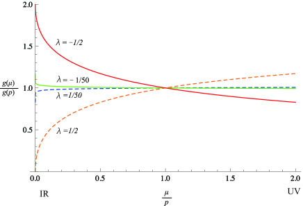
Figure 1: The evolution of the dimensionless constant $g(\mu)$ for $\lambda=1/50,1/2,-1/2,-1/50$.

Equation (34) reveals that only when

$$\frac{\lambda}{\tilde{C}}<0\,,$$ (35)

the RG flow has two FPs at $g(\mu)=0$ and $g(\mu)=-2\lambda/\tilde{C}$. In this case, the RG equation (34) can be solved as

$$g(\mu)=\frac{2}{1+\left(\mu\over p\right)^{\lambda}}\left(\mu\over p\right)^{\lambda}g(p)\,,$$ (36)

with

$$g(p)\equiv-\frac{\lambda}{\tilde{C}}\,,$$ (37)

where a pivot scale $p$ is introduced as an integration constant. In the case with $\lambda<0$, the coupling constant $g(\mu)$ flows from $0$ in the UV to $2g(p)$ in the IR. On the other hand, in the case with $\lambda>0$, the coupling constant $g(\mu)$ flows from $2g(p)$ in the UV to $0$ in the IR. Figure 1 shows the evolution of $g(\mu)$ for both positive and negative values of $\lambda$.

4 Deriving the $\zeta$ correlators

In this section, we consider the boundary QFT in the presence of the curvature perturbation $\zeta$, playing the role of an external source. Then, using the generating functional for the deformed conformal field theory, we will derive the relation between the vertex function $W^{(n)}(\hbox{\boldmath{$x$}}_{1},\,\cdots,\,\hbox{\boldmath{$x$}}_{n})$ and the correlation functions of the boundary operator $O$ in flat space.

4.1 Gauge conditions

In cosmological perturbation theory, the freedom to choose coordinates is usually referred to as gauge freedom. This corresponds to a choice of the time slicing, and with the choice of spatial coordinates on each slice. In the holographic description, we may think of a constant time slice as a holographic plane in which the QFT lives, while different times correspond to different values of the renormalization scale. Correlators of the gauge invariant variable $\zeta$ should be independent of the gauge choice (see also the discussion in Ref. [12]).

As the dictionary which relates the bulk and the boundary, in this paper, we assume that the coupling constant $g$ is related to the inflaton as

$$g(\mu,\,\hbox{\boldmath{$x$}})=\phi(t(\mu),\,\hbox{\boldmath{$x$}})\,,$$ (38)

where we set $M_{\rm pl}=1$. Since we assumed that the renormalization scale $\mu$ in the boundary is associated with the time coordinate $t$ in the bulk, we wrote the time coordinate of $\phi$ as $t(\mu)$. Equation (38) does not provide any restriction on the bulk dynamics, since we are not specifying the form of the kinetic term for $\phi$, or its potential. One may be interested in using more general function $g[\phi]$ instead of the linear one (38), but this can be understood simply as a change of variable which should not change the physics.

In the following, we compute the correlators of $\zeta$, using two gauges. In one gauge, we choose the holographic plane by requiring

$$\delta u(t,\,\hbox{\boldmath{$x$}})=\delta g(t,\,\hbox{\boldmath{$x$}})=\delta\phi(t,\,\hbox{\boldmath{$x$}})=0\,,$$ (39)

and the spatial coordinates by requiring that the spatial metric should be in the form:

$$h_{ij}=a^{2}(t)e^{2{\cal R}(t,\,\hbox{\boldmath{\scriptsize$x$}})}\delta_{ij}\,,$$ (40)

where ${\cal R}$ is the curvature perturbation. In this paper, the tensor perturbation will be completely neglected. As in the standard CPT, we refer to this gauge as the uniform field gauge. By definition, the curvature perturbation in the uniform field gauge gives the gauge invariant perturbation $\zeta$, i.e.,

$$\zeta(t,\,\hbox{\boldmath{$x$}})={\cal R}(t,\,\hbox{\boldmath{$x$}})\big{|}_{\delta g=0}\,.$$ (41)

In the other gauge, we choose the slicing and the spatial coordinates, requesting

$${\cal R}(t,\,\hbox{\boldmath{$x$}})=0\,$$ (42)

and

$$h_{ij}=a^{2}(t)\delta_{ij}\,,$$ (43)

respectively. We refer to this gauge as the flat gauge. In the flat gauge, the scalar perturbation is described solely by the fluctuation of the coupling constant $\delta g(t,\,\hbox{\boldmath{$x$}})$. In the following, we denote the fluctuation $\delta g(t,\,\hbox{\boldmath{$x$}})$ in the gauge ${\cal R}(t,\,{\bf x})=0$ as

$$\delta g_{f}(t,\,{\hbox{\boldmath{$x$}}})\equiv\delta g(t,\,\hbox{\boldmath{$x$}})\big{|}_{{\cal R}=0}=\delta\phi(t,\,\hbox{\boldmath{$x$}})\big{|}_{{\cal R}=0}\,,$$ (44)

which is also gauge invariant.

In the standard cosmological perturbation theory, performing the gauge transformation, we find that the curvature perturbation in the uniform field gauge, $\zeta$, is related to the fluctuation of the inflaton in the flat gauge $\delta g_{f}$ as (see e.g. [12, 37])

$$\zeta=-\frac{H}{\dot{\phi}}\delta g_{f}+\frac{\varepsilon_{2}}{4}\left(\frac{H}{\dot{\phi}}\right)^{2}\delta g_{f}^{2}+\cdots\,.$$ (45)

Here we abbreviated the sub-leading terms at large scales, as well as higher orders in $\delta g_{f}$, and we used the horizon flow functions, defined as

$$\varepsilon_{n}\equiv\frac{1}{\varepsilon_{n-1}}\frac{{\rm d}}{{\rm d}\ln a}\varepsilon_{n-1}$$ (46)

for $n\geq 1$, with

$$\varepsilon_{1}\equiv\frac{1}{2}\frac{\dot{\phi}^{2}}{H^{2}}\,.$$ (47)

Notice that for the scalar field with the non-canonical kinetic term, our $\varepsilon_{1}$ does not coincide with the standard definition of the horizon flow functions, given by $\varepsilon_{1}=-\dot{H}/H^{2}$.

4.2 Renormalization and counterterms

To derive finite correlation functions, we need to perform renormalization. The studies based on the holographic renormalization provide the necessary counterterms and renormalized action in the bulk (see, for instance, Refs. [38, 39, 40, 41, 42]). Meanwhile, to derive the renormalized correlation functions based on the boundary computation, we need to introduce the counterterms and determine the renormalized action in the boundary theory. One may expect that the introduction of the counterterms will alter the boundary theory through the contributions of the following three different types:

1. Additive local contributions which are independent of the boundary operators. These are made out of invariants constructed from the sources.

2. Contributions proportional to the boundary operator $O$.

3. Contributions proportional to new operators $O_{a}$ with $a=1,\,2,\,\cdots$.

Here, we consider the counter terms which keep the boundary theory local. Contributions of the second type will correspond to the renormalization of the coupling constant $u$ or $g$. Contributions of the third type will take us to the multi-field case. In this paper, we disregard this possibility, concentrating in the one field case.

Choosing the uniform field gauge with $\delta g=0$, the generating functional for the boundary theory is expressed as

$$Z_{\rm QFT}[\zeta]=\int D\chi\,e^{-S_{\rm QFT}[\zeta,\,\chi]}$$ (48)

with the action for the boundary QFT given by

$$S_{\rm QFT}[\zeta,\,\chi]\equiv S_{\rm CFT}-\int{\rm d}^{d}\hbox{\boldmath{$x$}}e^{d\zeta(\hbox{\boldmath{\scriptsize$x$}})}g(\mu){\cal O}(\mu,\,\hbox{\boldmath{$x$}})+S_{\rm source}[\zeta].$$ (49)

For notational convenience, we introduced

$${\cal O}(\mu,\,\hbox{\boldmath{$x$}})\equiv\mu^{-\lambda}O(\mu,\,\hbox{\boldmath{$x$}})\,.$$ (50)

In the right-hand side of the action, we absorbed the scale factor which appears from the invariant volume into $g(\mu)$. The third term in Eq. (49) denotes the additive contributions of the first type. Note that this term can be factorized in the generating functional $W_{\rm QFT}=-\ln Z_{\rm QFT}[\zeta]$ as

$$W_{\rm QFT}[\zeta]=-\ln\left[\int D\chi e^{-S_{\rm CFT}-\int{\rm d}^{d}\hbox{\boldmath{\scriptsize$x$}}e^{d\zeta}g{\cal O}}\right]+S_{\rm source}[\zeta]\,.$$ (51)

Therefore, when we derive the vertex function $W^{(n)}$ by taking the derivative with respect to $\zeta$ as in Eq. (12), the derivative which operates on $S_{\rm source}[\zeta]$ gives only the disconnected product of the ultralocal term where all arguments $\hbox{\boldmath{$x$}}_{i}$s coincide and the correlators of ${\cal O}$ derived from the first term in the right hand side of Eq. (51). Since we are interested in connected diagrams, we focus on the contribution from the first term.

4.3 $\zeta$ correlators from gauge invariance

In this subsection, we will study the relation between the vertex function $W^{(n)}$ and the correlators of ${\cal O}$, focusing on the fact that in the single field model where the gauge invariance is preserved, the gauge-invariant variable $\zeta$ can be expressed as a functional of the gauge invariant variable $\delta g_{f}$, i.e., $\zeta=\zeta[\delta g_{f}]$ or inversely $\delta g_{f}=\delta g_{f}[\zeta]$. For the time being, we proceed our discussion without invoking the explicit form of $\zeta=\zeta[\delta g_{f}]$. Equation (12) states that the vertex function $W^{(n)}(\hbox{\boldmath{$x$}}_{1},\,\cdots,\,\hbox{\boldmath{$x$}}_{n})$ is given by the $n$-th derivative of the generating functional $W_{\rm QFT}=-\ln Z_{\rm QFT}$. Recasting the derivative with respect to $\zeta$ into the derivative with respect to $\delta g_{f}$ by using the schematic relation $\delta g_{f}=\delta g_{f}[\zeta]$, we obtain

$$\frac{\delta W_{\rm QFT}}{\delta\zeta(\hbox{\boldmath{$x$}})}=\int{\rm d}^{d}\hbox{\boldmath{$y$}}\frac{\delta g_{f}(\hbox{\boldmath{$y$}})}{\delta\zeta(\hbox{\boldmath{$x$}})}\frac{\delta W_{\rm QFT}}{\delta g_{f}(\hbox{\boldmath{$y$}})}\,.$$ (52)

When $\delta g_{f}(\hbox{\boldmath{$x$}})$ is locally related to $\zeta(\hbox{\boldmath{$x$}})$ as in the large scale limit as given in Eq. (45), using Eq. (38), we find that $\delta g_{f}(\hbox{\boldmath{$x$}})$ is also related to $\zeta(\hbox{\boldmath{$x$}})$ locally. Then, we can rewrite Eq. (52) as

$$\frac{\delta W_{\rm QFT}}{\delta\zeta(\hbox{\boldmath{$x$}})}=-B(\hbox{\boldmath{$x$}})\frac{\delta W_{\rm QFT}}{\delta g_{f}(\hbox{\boldmath{$x$}})}\,,$$ (53)

where we introduced $B(\hbox{\boldmath{$x$}})$ as

$$B(\hbox{\boldmath{$x$}})\equiv-\frac{\partial\delta g_{f}(\hbox{\boldmath{$x$}})}{\partial\zeta(\hbox{\boldmath{$x$}})}\,.$$ (54)

Note that Eq. (53) states that taking the derivative with respect to the gauge invariant variable $\zeta$ is equivalent to taking the derivative with respect to $\delta g_{f}$ up to the factor $-B(\hbox{\boldmath{$x$}})$.

Next, using Eq. (53), we derive the relation between the vertex function $W^{(n)}$ and the correlators of ${\cal O}$ in the flat space. Taking the derivative of Eq. (53) with respect to $\zeta(\hbox{\boldmath{$x$}})$, we obtain

$$\frac{\delta^{2}W_{\rm QFT}}{\delta\zeta(\hbox{\boldmath{$x$}}_{1})\delta\zeta(\hbox{\boldmath{$x$}}_{2})}=B(\hbox{\boldmath{$x$}}_{1})B(\hbox{\boldmath{$x$}}_{2})\frac{\delta^{2}W_{\rm QFT}}{\delta g_{f}(\hbox{\boldmath{$x$}}_{1})\delta g_{f}(\hbox{\boldmath{$x$}}_{2})}-\frac{\delta B(\hbox{\boldmath{$x$}}_{1})}{\delta\zeta(\hbox{\boldmath{$x$}}_{2})}\frac{\delta W_{\rm QFT}}{\delta g_{f}(\hbox{\boldmath{$x$}}_{1})}\,.$$ (55)

Using Eqs. (12), (55), and

$$\frac{\delta^{n}W_{\rm QFT}}{\delta g_{f}(\hbox{\boldmath{$x$}}_{1})\cdots\delta g_{f}(\hbox{\boldmath{$x$}}_{n})}\bigg{|}_{\delta g_{f}=0}=(-1)^{n+1}\langle{\cal O}(\hbox{\boldmath{$x$}}_{1})\cdots{\cal O}(\hbox{\boldmath{$x$}}_{n})\rangle_{\mu}\,,$$ (56)

we obtain

$$W^{(2)}(\hbox{\boldmath{$x$}}_{1},\,\hbox{\boldmath{$x$}}_{2}) =-2{\rm Re}\left[B_{1}^{2}\langle{\cal O}(\hbox{\boldmath{$x$}}_{1}){\cal O}(\hbox{\boldmath{$x$}}_{2})\rangle_{\mu}\right]\,,$$ (57)

where we set the renormalization condition such that the ultralocal term with $\delta(\hbox{\boldmath{$x$}}_{1}-\hbox{\boldmath{$x$}}_{2})$ is canceled by the contribution from the quadratic term in $S_{\rm source}[\zeta]$. Here, introducing the $\mu$ dependent function $B_{n}(\mu)$ as

$$B_{n}(\mu)\equiv-\frac{\partial^{n}\delta g_{f}(\mu,\,\hbox{\boldmath{$x$}})}{\partial\zeta^{n}(\mu,\,\hbox{\boldmath{$x$}})}\bigg{|}_{\zeta=0}\,,$$ (58)

we expressed $B(\hbox{\boldmath{$x$}})$ as

$$B(\hbox{\boldmath{$x$}})\big{|}_{\zeta=0}=B_{1}(\mu)\,.$$ (59)

The vertex function $W^{(n)}$ with $n\geq 3$ can be obtained similarly and we find that $W^{(n)}$ is given in the form

$$W^{(n)}(\hbox{\boldmath{$x$}}_{1},\,\cdots,\,\hbox{\boldmath{$x$}}_{n})$$ (60)

$$=-2{\rm Re}\Bigl{[}B_{1}^{n}\langle{\cal O}(\hbox{\boldmath{$x$}}_{1})\cdots{\cal O}(\hbox{\boldmath{$x$}}_{n})\rangle_{\mu}$$ (61)

$$\qquad\qquad\,\,+B_{2}B_{1}^{n-2}\left\{\delta(\hbox{\boldmath{$x$}}_{1}-\hbox{\boldmath{$x$}}_{2})\langle{\cal O}(\hbox{\boldmath{$x$}}_{2})\cdots{\cal O}(\hbox{\boldmath{$x$}}_{n})\rangle_{\mu}+\left({\rm cyclic~{}perms}\right)\right\}+\cdots$$ (62)

$$\qquad\qquad\,\,+\!\sum_{m=1}^{[n/2]}\!B_{m}B_{n-m}\bigl{\{}\delta(\hbox{\boldmath{$x$}}_{1}-\hbox{\boldmath{$x$}}_{2})\cdots\delta(\hbox{\boldmath{$x$}}_{m-1}-\hbox{\boldmath{$x$}}_{m})\delta(\hbox{\boldmath{$x$}}_{m+1}-\hbox{\boldmath{$x$}}_{m+2})\cdots\delta(\hbox{\boldmath{$x$}}_{n-1}-\hbox{\boldmath{$x$}}_{n})$$ (63)

$$\qquad\qquad\qquad\qquad\qquad\qquad\qquad\times\langle{\cal O}(\hbox{\boldmath{$x$}}_{m}){\cal O}(\hbox{\boldmath{$x$}}_{m+1})\rangle_{\mu}+\left({\rm cyclic~{}perms}\right)\bigr{\}}\Bigr{]}\,,$$ (64)

where $[x]$ denotes the Gauss’s floor function. Here, the delta functions appeared by taking the derivative of $B(\hbox{\boldmath{$x$}})$ with respect to $\zeta(\hbox{\boldmath{$x$}})$, for instance, as

$$\frac{\delta B(\hbox{\boldmath{$x$}}_{1})}{\delta\zeta(\hbox{\boldmath{$x$}}_{2})}\bigg{|}_{\zeta=0}=\delta(\hbox{\boldmath{$x$}}_{1}-\hbox{\boldmath{$x$}}_{2})B_{2}(\mu)\,.$$

In Eq. (64), we again eliminated the ultralocal term, using the contribution from the $n$-th term in $S_{\rm source}[\zeta]$. Once the relation between $\delta\phi$ and $\zeta$ is given, using Eq. (64), we can express the vertex function $W^{(n)}$ by $B_{n}$ and the correlators of ${\cal O}$ in the flat space. Namely, when we use the relation (45), we can express $B_{n}$ as

$$B_{1}=\frac{\dot{\phi}}{H}=\frac{{\rm d}\phi}{{\rm d}\ln a}\,,$$ (65)

$$B_{2}=-\frac{\dot{\phi}}{H}\frac{\varepsilon_{2}}{2}=-\frac{{\rm d}B_{1}}{{\rm d}\ln a}=-\frac{{\rm d}^{2}\phi}{{\rm d}\ln a^{2}}\,.$$ (66)

Thus, the relation between the vertex function $W^{(n)}$ and the correlators of ${\cal O}$ is specified by invoking the relation between $\zeta$ and $\delta g_{f}$, derived by performing the gauge transformation in the cosmological perturbation theory. In Appendix B, we seek for an alternative way to relate $W^{(n)}$ to the correlators of ${\cal O}$. The ambiguity discussed in Appendix B.2 can be eliminated by using the relation (45).

5 Conservation of the curvature perturbation $\zeta$

In this section, after we overview the discussion about the conservation of the curvature perturbation $\zeta$ based on the standard CPT, we address the conservation of the curvature perturbation from holography.

5.1 Conservation in the standard cosmological perturbation theory

In cosmological perturbation theory (CPT) the conservation of the curvature perturbation $\zeta$ holds in the large scale limit for the adiabatic time evolution, when the matter content is dominated by a single species  [43, 44, 45, 46, 47]. This is useful, for instance, in order to evolve the predicted distribution function for $\zeta$ through the process of reheating, the details of which are largely unknown. For a barotropic perfect fluid, the conservation of $\zeta$ at large scales can be derived directly from the conservation of the energy momentum tensor, without invoking the theory of gravity. In turn, the conservation of the energy momentum tensor in a local theory just relies on the equivalence principle, usually implemented through general covariance.

Since the validity of the conservation of $\zeta$ is so generic, any evidence that conservation is violated can provide some useful insight on the nature of the underlying theory of inflation. In the following subsection, we will study the validity of the conservation of $\zeta$ based on the boundary computation. Before that, let us briefly summarize the discussion based on the standard CPT. (The conservation of $\zeta$ has been mostly discussed for $d=3$, so in this section, we consider $d=3$. However, it will hold also in other dimensions.)

In Ref. [44], Wands et al. showed the conservation of $\zeta$ for the barotropic fluid, whose energy density perturbation $\delta\rho$ is proportional to the pressure perturbation $\delta p$, at linear order in perturbation. Using the energy conservation equation $n^{\nu}T^{\mu}\!_{\nu;\mu}=0$ with the unit timelike vector $n^{\nu}$:

$$\delta\dot{\rho}=-3H(\delta\rho+\delta p)-3\dot{{\cal R}}(\rho+p)+O\left((k/aH)^{2}\right)\,,$$ (67)

where $\rho$ and $p$ are the background values of the energy density and the pressure, they found that in the uniform density gauge $\delta\rho=0$, the curvature perturbation is conserved in time at large scales. This argument was extended to the non-linear order by Lyth et al. based on the gradient expansion in Ref. [46] and also by Langlois and Vernizzi based on the covariant approach in Ref. [47]. Their arguments proceed independent of the theory of gravitation in the bulk.

Note that when we consider the scalar field, the adiabatic condition, that states the pressure is expressed only by the energy density, becomes less clear. In fact, even in the single field case, the adiabatic condition is not necessarily satisfied. In Ref. [48], Naruko and Sasaki considered the Galileon-type scalar field whose equation of motion involves up to the first derivative of the metric. Then, using the equation of motion with the aid of the gradient expansion, they showed that in the attractor phase, during which the equation of motion for $\phi$ becomes the first order as $\dot{\phi}=f(\phi)$, the uniform field gauge can be chosen and the curvature perturbation in this gauge, $\zeta$, is conserved at large scales. (See also Ref. [49].) So far, we have summarized the discussions about the classical evolution which does not include the loop corrections. The conservation of $\zeta$ is discussed also in the presence of loop corrections [50, 51], but the validity of the conservation for the loop corrections is still unclear [52, 53].

5.2 Conservation from holography?

In this subsection, we investigate the conservation of the gauge-invariant curvature perturbation $\zeta$ based on holography. In holography, the conservation of $\zeta$ can be addressed by studying the $\mu$ dependence, which is interpreted as the time dependence in the cosmological evolution. Notice that since the renormalized theory, obtained after integrating out the UV modes, consists only the wavenumber $k$ with $k<\mu$, the correlators of $\zeta$ given by the renormalized boundary theory will describe the evolution of $\zeta$ at large scales.

Here, we note that the $n$-point function of $\zeta$ is described solely in terms of the vertex functions $W^{(m)}$ with $m\leq n$. For instance, as is shown in Ref. [20], the power spectrum of $\zeta$ is given by

$$\langle\zeta(\hbox{\boldmath{$x$}}_{1})\zeta(\hbox{\boldmath{$x$}}_{2})\rangle_{\rm conn}=W^{(2)\,-1}(\hbox{\boldmath{$x$}}_{1},\,\hbox{\boldmath{$x$}}_{2})\,,$$ (68)

with the inverse matrix of $W^{(2)}(\hbox{\boldmath{$x$}}_{1},\,\hbox{\boldmath{$x$}}_{2})$, and the bi-spectrum is given by

$$\langle\zeta(\hbox{\boldmath{$x$}}_{1})\zeta(\hbox{\boldmath{$x$}}_{2})\zeta(\hbox{\boldmath{$x$}}_{3})\rangle_{\rm conn}=-\int\prod_{i=1}^{3}{\rm d}^{d}\hbox{\boldmath{$y$}}_{i}\,W^{(2)\,-1}(\hbox{\boldmath{$x$}}_{i}\,,\hbox{\boldmath{$y$}}_{i})\,W^{(3)}(\hbox{\boldmath{$y$}}_{1},\,\hbox{\boldmath{$y$}}_{2},\,\hbox{\boldmath{$y$}}_{3})\,.$$ (69)

To make the power spectrum of $\zeta$ conserved, the vertex function $W^{(2)}$ should be independent of $\mu$. Given that the power spectrum is conserved, to further make the bi-spectrum of $\zeta$ conserved, the vertex function $W^{(3)}$ should be also independent of $\mu$. Thus, to make all the $m$-point functions of $\zeta$ with $m\leq n$ conserved, the vertex functions $W^{(m)}$ with $m\leq n$ should be totally independent of $\mu$. Therefore, in the following, we study the $\mu$ dependence of the vertex function $W^{(n)}$.

In this subsection, we study whether the correlators of $\zeta$ become $\mu$ independent or not under the following two assumptions:

• The gauge invariant variables $\zeta$ and $\delta g_{f}$ are locally related schematically as

  $$\zeta(\hbox{\boldmath{$x$}})=\zeta[\delta g_{f}(\hbox{\boldmath{$x$}})]\,.$$ (70)

• The dual boundary theory can be renormalized by using the wave function renormalization $Z(\mu)$ as

  $$Z^{-n/2}(\mu)\langle{\cal O}(\hbox{\boldmath{$x$}}_{1})\cdots{\cal O}(\hbox{\boldmath{$x$}}_{n})\rangle_{\mu}=Z^{-n/2}(\mu_{0})\langle{\cal O}(\hbox{\boldmath{$x$}}_{1})\cdots{\cal O}(\hbox{\boldmath{$x$}}_{n})\rangle_{\mu_{0}}\,.$$ (71)

The first assumption will hold generally at large scales (see for instance Eq. (45)), unless a non-local operator, which typically gives rise to the singular pole in the limit $k\to 0$, shows up in the relation between $\zeta$ and $\delta g_{f}$.

In Sec. 4.3, using Eq. (70), we derived the vertex function $W^{(n)}$ as in Eq. (64). First, we consider the power spectrum, given by the inverse matrix of

$$W^{(2)}(\hbox{\boldmath{$x$}}_{1},\,\hbox{\boldmath{$x$}}_{2}) =-2{\rm Re}\left[B_{1}^{2}(\mu)\langle{\cal O}(\hbox{\boldmath{$x$}}_{1}){\cal O}(\hbox{\boldmath{$x$}}_{2})\rangle_{\mu}\right]\,.$$ (72)

Inserting Eq. (71) into Eq. (72), we find that to make $W^{(2)}$ independent of $\mu$, the wave function renormalization $Z(\mu)$ should satisfy

$$\frac{{\rm d}}{{\rm d}\mu}\left[B_{1}(\mu)\sqrt{Z(\mu)}\right]=0\,.$$ (73)

Next, we consider the bi-spectrum of $\zeta$, expressed by $W^{(2)\,-1}$ and

$$W^{(3)}(\hbox{\boldmath{$x$}}_{1},\,\hbox{\boldmath{$x$}}_{2},\,\hbox{\boldmath{$x$}}_{3})$$ (74)

$$=-2{\rm Re}\Bigl{[}B_{1}^{3}(\mu)\langle{\cal O}(\hbox{\boldmath{$x$}}_{1}){\cal O}(\hbox{\boldmath{$x$}}_{2}){\cal O}(\hbox{\boldmath{$x$}}_{3})\rangle_{\mu}$$ (75)

$$\qquad\quad\qquad+B_{2}(\mu)B_{1}(\mu)\left\{\delta(\hbox{\boldmath{$x$}}_{1}-\hbox{\boldmath{$x$}}_{2})\langle{\cal O}(\hbox{\boldmath{$x$}}_{2}){\cal O}(\hbox{\boldmath{$x$}}_{3})\rangle_{\mu}+\left({\rm cyclic~{}perms}\right)\right\}\Bigr{]}\,.$$ (76)

When the condition (73) is fulfilled, the first term in the right-hand side of Eq. (76) becomes $\mu$ independent. In addition, to make the terms in the third line of Eq. (76) independent of $\mu$, $B_{2}(\mu)$ should be given as

$$B_{2}(\mu)=s_{2}B_{1}(\mu)$$ (77)

with a constant parameter $s_{2}$. Note that using Eq. (66), we can express the parameter $s_{2}$ as

$$s_{2}=-\frac{{\rm d}}{{\rm d}\ln a}\ln B_{1}\,.$$ (78)

Repeating a similar argument, we find that only if the condition (73) is satisfied and $B_{m}(\mu)$ with $m\leq n$ is given as

$$B_{m}(\mu)=s_{m}B_{1}(\mu)$$ (79)

with a constant parameter $s_{m}$, the vertex function $W^{(n)}$ becomes independent of $\mu$, implying the conservation of $\zeta$.

Next, we examine whether the conditions (73) and (79) can be fulfilled, solving the RG flow explicitly. In Appendix A, following Ref. [30], we computed the renormalized correlators of ${\cal O}$ and then the wave function renormalization is given as

$$\sqrt{Z(\mu)}=\mu^{-\lambda}\left[1+\Bigl{(}\frac{\mu}{p}\Bigr{)}^{\lambda}\right]^{2}=4p^{-\lambda}\frac{\beta(p)}{\beta(\mu)}\,.$$ (80)

(The wave function renormalization is discussed from a different perspective in Ref. [54].) On the second equality, we noted that using Eqs. (33) and (36), the beta function is given as

$$\beta(\mu)=\frac{4}{\Bigl{[}1+\left(\mu\over p\right)^{\lambda}\Bigr{]}^{2}}\left(\mu\over p\right)^{\lambda}\beta(p)=\frac{\lambda}{1+\left(\mu\over p\right)^{\lambda}}g(\mu)\,,$$ (81)

with

$$\beta(p)\equiv\frac{\lambda}{2}g(p)\,.$$ (82)

Using Eq. (80), we find that the condition (73) implies

$$B_{1}(\mu)={\cal C}\beta(\mu)\,,$$ (83)

where ${\cal C}$ is a constant parameter. When we use the relation (45) derived by performing the gauge transformation, the $\mu$ dependent functions $B_{1}$ and $B_{2}$ are given as in Eqs. (65) and (66). Using Eqs. (33), (65), and (83), we find that the renormalization scale $\mu$ should be related to the time coordinate in cosmology as

$$\ln(\mu/\mu_{0})={\cal C}\ln(a/a_{0})\,,$$ (84)

where $a_{0}$ denotes the scale factor at the time associated with $\mu_{0}$. When the RG flow has the conformal FP, since $\mu$ is proportional to $a$ near the FP [30, 32, 33, 34], ${\cal C}$ should be set to 1.

On the other hand, we find that in general the second condition (79) cannot be fulfilled. In fact, using Eqs. (83) and (84), we obtain

$$s_{2}=-{\cal C}\frac{{\rm d}}{{\rm d}\ln\mu}\ln\beta\,,$$ (85)

which can be solved as

$$\beta(\mu)=\beta_{0}\left(\mu\over\mu_{0}\right)^{\lambda}\,,$$ (86)

with the constant $\lambda=\Delta-d$ given by

$$\lambda=-\frac{s_{2}}{{\cal C}}\,.$$ (87)

Therefore, unless we consider the RG flow which has the constant scaling dimension as in Eq. (86), the condition (83) cannot be fulfilled along the entire RG flow. It is clear that the beta function for the RG flow with the two FPs (81) deviates from Eq. (86) once away from the FPs and then we find Eq. (83) cannot be satisfied except for the vicinities of the IR and UV FPs. When the right hand side of Eq. (85) ceases to be constant, the bi-spectrum of $\zeta$, namely the terms in the last line of Eq. (76), can evolve even at large scales, contradicting the prediction of the CPT for the single field models of inflation.

Several comments are in order regarding the RG flow whose beta function is given by Eq. (86). This RG flow has at most one FP: not having any FP or having only one FP either in the IR or UV. Using Eq. (84), we can rewrite Eq. (86) in terms of the cosmological quantities as

$$\beta(a)=\frac{1}{{\cal C}}\frac{{\rm d}\phi}{{\rm d}\ln a}=\beta_{0}\left(a\over a_{0}\right)^{-s_{2}}\,.$$ (88)

Notice that Eq. (88) restricts the evolution of $\phi(a)$ and also the potential $V(\phi)$, indicating that the conservation of $\zeta$ can be verified only for the specific single field model of inflation.

When $\beta(\mu)$ is given by Eq. (86), $\beta(\mu)$ yields the RG equation (34) with $\lambda=-s_{2}/{\cal C}$ and $C=0$. In this case, the two-point function of ${\cal O}$ is simply given by

$$\langle{\cal O}(\hbox{\boldmath{$x$}}_{1}){\cal O}(\hbox{\boldmath{$x$}}_{2})\rangle_{\mu}=\left(\mu\over\mu_{0}\right)^{-2\lambda}\frac{c_{0}}{|\hbox{\boldmath{$x$}}_{1}-\hbox{\boldmath{$x$}}_{2}|^{2(\lambda+3)}}\,,$$ (89)

where $c_{0}$ is a constant parameter. Inserting Eqs. (86) and (89) into Eq. (72), we obtain the vertex function $W^{(2)}$ as

$$W^{(2)}(\hbox{\boldmath{$x$}}_{1},\,\hbox{\boldmath{$x$}}_{2})=-\frac{2{\cal C}^{2}\beta^{2}_{0}c_{0}}{|\hbox{\boldmath{$x$}}_{1}-\hbox{\boldmath{$x$}}_{2}|^{2(\lambda+3)}}\,.$$ (90)

Using Eqs. (68) and (90), we obtain the power spectrum of $\zeta$ as

$$P_{\zeta}(k)=-\frac{6}{\pi^{2}}\frac{1}{{\cal C}^{2}\beta^{2}_{0}c_{0}}\frac{1}{k^{3+2\lambda}}\,.$$ (91)

Thus, the amplitude and the spectral tilt of $\zeta$ are expressed by $\beta_{0}$, ${\cal C}$, and $\lambda=-s_{2}/{\cal C}$. Notice that Eq. (91) states that to provide a red-tilted spectrum which is consistent with the observation of the cosmic microwave background, $\lambda=-s_{2}/{\cal C}$ should be positive. In that case, the beta function blows up in the UV, causing the breakdown of conformal perturbation theory at sufficiently short distances.

6 Discussion

In this paper, we examined whether the curvature perturbation $\zeta$ is conserved under the change of $\mu$ in a local boundary theory with the action (49). This corresponds to a generic CFT with a single deformation operator.

In order to relate the boundary correlators to the correlators of the gauge invariant curvature perturbation $\zeta$, we have assumed that $\zeta$ is locally related to the scalar field perturbation in the flat gauge, $\delta\phi_{f}$ (or equivalently the perturbation of the coupling $\delta g_{f}$) as in Eq. (70). This assumption certainly holds in standard cosmological perturbation theory at large scales. Also, we have assumed that the boundary operator ${\cal O}$ is renormalized multiplicatively as in Eq. (71). Solving the RG flow, we found that the power spectrum of $\zeta$ is conserved if we identify the renormalization scale $\mu$ with the scale factor $a$ in the bulk, as in Eq. (84). But then, it follows that the bi-spectrum of $\zeta$ cannot be conserved along the entire RG flow. The only exception is the particular case where the scaling dimension is constant, as given in Eq. (86). This special case leads to an exact power law spectrum of the form (91).

In order to have conservation of $\zeta$ along a generic RG flow, we need to abandon at least one of the following three assumptions: the local relation Eq. (70), the multiplicative renormalization Eq. (71) or the assumption of a local boundary theory with the single deformation operator.

The local relation Eq. (70) follows from Eqs. (38) and (45). Instead of imposing Eq. (38), one may need to seek for a more non-trivial relation between $g$ and $\phi$ (this issue has been discussed in AdS/CFT. See, for instance, Ref. [55]). A simple generalization to the local function $g(\mu,\,\hbox{\boldmath{$x$}})=g[\phi(t(\mu),\,\hbox{\boldmath{$x$}})]$ is just a change of variable describing the field, and will not help to preserve the conservation. The second and third assumptions are concerned with renormalization. In this paper, we assumed that the boundary QFT can be renormalized by introducing the counterterm and the wave function renormalization as in Eqs. (49) and (71), respectively. Nevertheless, in general, one may need to introduce more than one deformation operator to perform the renormalization. In addition, the QFT may become non-local after the renormalization. These cases were not addressed in the present paper. When the boundary theory contains more than one deformation operator, the corresponding cosmological evolution will be governed by several scalar fields. Notice, however, that in this case the standard CPT does not predict the conservation of $\zeta$ any longer. The possibility of generalizing the duality to the case of a non-local boundary theory is at present not very well understood. In particular, it is not clear whether the locality (non-locality) in one side of the duality implies the locality (non-locality) on the other side. A relevant discussion can be found in Ref. [56], but to our knowledge this issue has not been fully resolved, at least in the case when the deviation from dS spacetime becomes important (even in the large $N$ limit). If a non-local boundary theory can be dual to a local bulk theory with a single field, the conservation of $\zeta$ should be predicted also from the boundary computation. We leave this issue for future research.

In this paper, we discussed the asymptotically dS spacetimes and the dual boundary QFT. Since the asymptotically dS spacetimes which we have considered can be transformed into the asymptotically AdS spacetime by analytic continuation, the analog of $\zeta$ will be conserved along the holographic direction also in the case of asymptotically AdS spacetimes. Possible implications of our results in this broader context are currently under investigation.

Appendix A Correlators of the boundary operator $O$

In this section, we compute the renormalized $n$-point functions of $O$. Following Ref. [30], we perform the renormalization in the conventional way, introducing the UV cutoff. Expanding the $n$-point function regarding the deformation term $\int{\rm d}^{d}\hbox{\boldmath{$x$}}uO$ as

$$\langle O(\hbox{\boldmath{$x$}}_{1})\cdots O(\hbox{\boldmath{$x$}}_{n})\rangle_{\mu}$$ (92)

$$=\sum_{m=0}^{\infty}\frac{1}{m!}(-u)^{m}\int{\rm d}^{d}\hbox{\boldmath{$y$}}_{1}\cdots\int{\rm d}^{d}\hbox{\boldmath{$y$}}_{m}\langle O(\hbox{\boldmath{$x$}}_{1})\cdots O(\hbox{\boldmath{$x$}}_{n})O(\hbox{\boldmath{$y$}}_{1})\cdots O(\hbox{\boldmath{$y$}}_{m})\rangle_{\mu,\,0}\,,$$ (93)

we express the $n$-point function as the summation of the correlators for the “CFT” with the cutoff at $\mu$ (here we put the quotes since the theory cannot be the exact CFT due to the presence of the cutoff), which we denote as $\langle\cdots\rangle_{\mu,\,0}$. We first compute

$$I_{m}^{(n)}(\hbox{\boldmath{$x$}}_{1},\,\cdots,\,\hbox{\boldmath{$x$}}_{n},\,\mu)$$ (94)

$$\equiv\int{\rm d}^{d}\hbox{\boldmath{$y$}}_{1}\cdots\int{\rm d}^{d}\hbox{\boldmath{$y$}}_{m}\langle O(\hbox{\boldmath{$x$}}_{1})\cdots O(\hbox{\boldmath{$x$}}_{n})O(\hbox{\boldmath{$y$}}_{1})\cdots O(\hbox{\boldmath{$y$}}_{m})\rangle_{\mu,\,0}\,.$$ (95)

Note that since this is the correlators with the cutoff $\mu$, all the points $z$ and $\hbox{\boldmath{$z$}}^{\prime}$ which are either $\hbox{\boldmath{$x$}}_{i}$ with $i=1,\cdots,\,n$ or $\hbox{\boldmath{$y$}}_{i}$ with $i=1,\cdots,\,m$ should satisfy

$$|\hbox{\boldmath{$z$}}-\hbox{\boldmath{$z$}}^{\prime}|\geq 1/\mu\,.$$ (96)

First, we compute $I^{(n)}_{1}$, which is given as

$$I_{1}^{(n)}(\hbox{\boldmath{$x$}}_{1},\,\cdots,\,\hbox{\boldmath{$x$}}_{n},\mu)$$ (97)

$$=\int{\rm d}^{d}\hbox{\boldmath{$y$}}\langle O(\hbox{\boldmath{$x$}}_{1})\cdots O(\hbox{\boldmath{$x$}}_{n})O(\hbox{\boldmath{$y$}})\rangle_{\mu,\,0}\prod^{n}_{i=1}\theta\left(|\hbox{\boldmath{$x$}}_{i}-\hbox{\boldmath{$y$}}|-1/\mu\right)\,,$$ (98)

beginning at $\mu=\mu_{0}$ as in Sec. 3.2. Here, using the Heaviside function, we explicitly described the condition (96). Then, changing the cutoff from $\mu_{0}$ to $\mu$, we obtain the change of $I_{1}^{(n)}$ as

$$\Delta I_{1}^{(n)}(\hbox{\boldmath{$x$}}_{1},\,\cdots,\,\hbox{\boldmath{$x$}}_{n},\,\mu)$$ (99)

$$=-\int{\rm d}^{d}\hbox{\boldmath{$y$}}\langle O(\hbox{\boldmath{$x$}}_{1})\cdots O(\hbox{\boldmath{$x$}}_{n})O(\hbox{\boldmath{$y$}})\rangle_{\mu,\,0}\sum^{n}_{i=1}\delta\left(|\hbox{\boldmath{$x$}}_{i}-\hbox{\boldmath{$y$}}|-1/\mu\right)\Delta\!\left(1\over\mu\right)\,,$$ (100)

where we replaced the remaining Heaviside functions which we didn’t take differentiation with $1$. Taking the infinitesimal limit, we obtain

$$\mu\frac{{\rm d}}{{\rm d}\mu}I_{1}^{(n)}(\hbox{\boldmath{$x$}}_{1},\,\cdots,\,\hbox{\boldmath{$x$}}_{n},\,\mu)$$ (101)

$$\,\,=\mu^{-1}\int{\rm d}^{d}\hbox{\boldmath{$y$}}\langle O(\hbox{\boldmath{$x$}}_{1})\cdots O(\hbox{\boldmath{$x$}}_{n})O(\hbox{\boldmath{$y$}})\rangle_{\mu,\,0}\sum^{n}_{i=1}\delta\left(|\hbox{\boldmath{$x$}}_{i}-\hbox{\boldmath{$y$}}|-1/\mu\right)\,.$$ (102)

Using the OPE, given in Eq. (18), we rewrite the right-hand side as

$$\langle O(\hbox{\boldmath{$x$}}_{1})\cdots O(\hbox{\boldmath{$x$}}_{n})O(\hbox{\boldmath{$y$}})\rangle_{\mu,\,0}\,\delta\left(|\hbox{\boldmath{$x$}}_{1}-\hbox{\boldmath{$y$}}|-1/\mu\right)$$ (103)

$$\,=\frac{C}{c}\frac{1}{|\hbox{\boldmath{$x$}}_{1}-\hbox{\boldmath{$y$}}|^{\Delta_{0}}}\langle O(\hbox{\boldmath{$x$}}_{1})\cdots O(\hbox{\boldmath{$x$}}_{n})\rangle_{\mu,\,0}\,\delta\left(|\hbox{\boldmath{$x$}}_{1}-\hbox{\boldmath{$y$}}|-1/\mu\right)+\cdots\,,$$ (104)

where the first term in the OPE (18) should be eliminated by introducing the counter term and the ellipsis denotes the non-singular terms in the limit $|\hbox{\boldmath{$x$}}_{1}-\hbox{\boldmath{$y$}}|\to 0$. Here, $\Delta_{0}$ denotes the scaling dimension at $\mu=\mu_{0}$. Then, integrating about $y$, we obtain

$$\mu\frac{{\rm d}}{{\rm d}\mu}I_{1}^{(n)}(\hbox{\boldmath{$x$}}_{1},\,\cdots,\,\hbox{\boldmath{$x$}}_{n},\,\mu)=n\tilde{C}\mu^{\lambda}I^{(n)}_{0}(\hbox{\boldmath{$x$}}_{1},\,\cdots,\,\hbox{\boldmath{$x$}}_{n})+\cdots\,,$$ (105)

where we introduced $\tilde{C}\equiv{\rm Vol}(S^{d-1})C/c$, $\lambda\equiv\lambda(\mu_{0})$, and

$$I_{0}^{(n)}(\hbox{\boldmath{$x$}}_{1},\,\cdots\hbox{\boldmath{$x$}}_{n})\equiv\langle O(\hbox{\boldmath{$x$}}_{1})\cdots O(\hbox{\boldmath{$x$}}_{n})\rangle_{0}\,.$$ (106)

Note that the non-singular terms in the OPE will be written in the form $|\hbox{\boldmath{$x$}}_{i}-\hbox{\boldmath{$y$}}|^{p}$ with a non-negative real number $p$, which will be replaced with $\mu^{-p}$ after integrating about $y$. Therefore, the contributions from the non-singular terms will be suppressed by $(r\mu)^{-(\Delta_{0}+p)}$ compared with the first term in Eq. (105), where $r$ is a scale associated with $I_{1}^{(n)}$, and hence we can neglect them in the large scale limit. Noticing the fact that $I^{(n)}_{0}$ is the correlator for the CFT, which does not vary in the change of $\mu$, we can solve Eq. (105) as

$$I_{1}^{(n)}(\hbox{\boldmath{$x$}}_{1},\,\cdots,\,\hbox{\boldmath{$x$}}_{n},\,\mu)=n\tilde{C}\,\frac{\mu^{\lambda}-(fr)^{-\lambda}}{\lambda}\,I_{0}^{(n)}(\hbox{\boldmath{$x$}}_{1},\,\cdots,\,\hbox{\boldmath{$x$}}_{n})\,,$$ (107)

where $f$ is a dimensionless constant. Since the two-point function for the “CFT” with the cutoff $\mu$ should agree with the one for the exact CFT, when the distance $x_{12}\equiv|\hbox{\boldmath{$x$}}_{1}-\hbox{\boldmath{$x$}}_{2}|$ is much bigger than $1/\mu$, the dimensionful parameter $r$ in $I_{1}^{(2)}$ should be $x_{12}$, which is the only dimensionful quantity included in the two-point function for the CFT. Then, we can determine $I_{1}^{(2)}(\hbox{\boldmath{$x$}}_{1},\,\hbox{\boldmath{$x$}}_{2},\,\mu)$ up to the constant parameter $f$ as

$$I_{1}^{(2)}(\hbox{\boldmath{$x$}}_{1},\,\hbox{\boldmath{$x$}}_{2},\,\mu)=2\tilde{C}\,\frac{\mu^{\lambda}-(fx_{12})^{-\lambda}}{\lambda}\,I_{0}^{(2)}(\hbox{\boldmath{$x$}}_{1},\,\hbox{\boldmath{$x$}}_{2})\,.$$ (108)

By contrast, for $n\geq 3$, $I_{1}^{(n)}$ can depend on all the distances $x_{ij}\equiv|\hbox{\boldmath{$x$}}_{i}-\hbox{\boldmath{$x$}}_{j}|$ with $i,j=1,\,\cdots,\,n$ and hence we cannot determine the term $(fr)^{-\lambda}$ only from the dimensional analysis. In the following, simply assuming that $(fr)^{-\lambda}$ should be expressed by a product of $x_{ij}$s, we use the formal expression (107).

Next, we compute $I^{(n)}_{m}(\hbox{\boldmath{$x$}}_{1},\,\cdots,\,\hbox{\boldmath{$x$}}_{n},\,\mu)$. Following a similar argument, we obtain

$$\mu\frac{{\rm d}}{{\rm d}\mu}I_{m}^{(n)}(\hbox{\boldmath{$x$}}_{1},\,\cdots,\,\hbox{\boldmath{$x$}}_{n},\,\mu)$$ (109)

$$=\mu^{-1}\int{\rm d}^{d}\hbox{\boldmath{$y$}}_{1}\cdots\int{\rm d}^{d}\hbox{\boldmath{$y$}}_{m}\langle O(\hbox{\boldmath{$x$}}_{1})\cdots O(\hbox{\boldmath{$x$}}_{n})O(\hbox{\boldmath{$y$}}_{1})\cdots O(\hbox{\boldmath{$y$}}_{m})\rangle_{\mu,\,0}$$ (110)

$$\qquad\qquad\times\left[\sum^{n}_{i=1}\sum_{j=1}^{m}\delta\left(|\hbox{\boldmath{$x$}}_{i}-\hbox{\boldmath{$y$}}_{j}|-1/\mu\right)+\sum_{j,\,j^{\prime}}\delta\left(|\hbox{\boldmath{$y$}}_{j}-\hbox{\boldmath{$y$}}_{j^{\prime}}|-1/\mu\right)\right]\,,$$ (111)

where the second term in the last line represents all the combinations about $j$ and $j^{\prime}$ with $j,j^{\prime}=1,\,\cdots,\,m$. Then, using the OPE (18) and integrating about one of $\hbox{\boldmath{$y$}}_{j}$ or $\hbox{\boldmath{$y$}}_{j^{\prime}}$ which appears in each accompanied delta function, we obtain

$$\mu\frac{{\rm d}}{{\rm d}\mu}I_{m}^{(n)}(\hbox{\boldmath{$x$}}_{1},\,\cdots,\,\hbox{\boldmath{$x$}}_{n},\,\mu)=B^{(n)}_{m}\,\tilde{C}\mu^{\lambda}\,I_{m-1}^{(n)}(\hbox{\boldmath{$x$}}_{1},\,\cdots,\,\hbox{\boldmath{$x$}}_{n},\,\mu)\,,$$ (112)

where we again neglected the non-singular contributions in the OPE and $B^{(n)}_{m}$ denotes the number of terms with the delta functions in the last line of Eq. (111), given by

$$B^{(n)}_{m}\equiv\frac{m}{2}(2n+m-1)\,.$$ (113)

Introducing $y(\mu)$ which satisfies

$$\frac{{\rm d}y(\mu)}{{\rm d}\mu}=\tilde{C}\mu^{\lambda-1}\,,$$ (114)

we rewrite Eq. (112) as

$$\frac{{\rm d}}{{\rm d}y}I_{m}^{(n)}(\hbox{\boldmath{$x$}}_{1},\,\cdots,\,\hbox{\boldmath{$x$}}_{n},\,y)=B^{(n)}_{m}\,I_{m-1}^{(n)}(\hbox{\boldmath{$x$}}_{1},\,\cdots,\,\hbox{\boldmath{$x$}}_{n},\,y)\,.$$ (115)

Operating ${\rm d}^{m-1}/{\rm d}y^{m-1}$, we obtain

$$\frac{{\rm d}^{m}}{{\rm d}y^{m}}I_{m}^{(n)}(\hbox{\boldmath{$x$}}_{1},\,\cdots,\,\hbox{\boldmath{$x$}}_{n},\,y)=\prod_{m^{\prime}=1}^{m}B^{(n)}_{m^{\prime}}\,I_{0}^{(n)}(\hbox{\boldmath{$x$}}_{1},\,\cdots,\,\hbox{\boldmath{$x$}}_{n})\,.$$ (116)

Note that, since $I^{(n)}_{0}$ is the $n$-point functions for the CFT, we can solve this equation as

$$I_{m}^{(n)}(\hbox{\boldmath{$x$}}_{1},\,\cdots,\,\hbox{\boldmath{$x$}}_{n},\,y)=\frac{1}{m!}\prod_{m^{\prime}=1}^{m}B^{(n)}_{m^{\prime}}\,I_{0}^{(n)}(\hbox{\boldmath{$x$}}_{1},\,\cdots,\,\hbox{\boldmath{$x$}}_{n})y^{m}+\sum_{m^{\prime}=0}^{m-1}d_{m^{\prime}}y^{m^{\prime}}\,,$$ (117)

where $d_{m^{\prime}}$ is constant in $y$, but can depend on $\hbox{\boldmath{$x$}}_{i}$ with $i=1,\,\cdots,\,n$. Inserting this solution into Eq. (115), we obtain

$$\sum_{m^{\prime}=0}^{m-2}(m^{\prime}+1)d_{m^{\prime}+1}y^{m^{\prime}}=B^{(n)}_{m}\sum_{m^{\prime}=0}^{m-2}d_{m^{\prime}}y^{m^{\prime}}\,.$$ (118)

Comparing the coefficients of $\chi^{m^{\prime}}$, we obtain

$$d_{m^{\prime}}=B^{(n)}_{m}\frac{d_{m^{\prime}-1}}{m^{\prime}}=\left\{B^{(n)}_{m}\right\}^{m^{\prime}}\frac{d_{0}}{m^{\prime}!}\,.$$ (119)

Inserting this expression into Eq. (117), we can solve

$$I_{m}^{(n)}(\hbox{\boldmath{$x$}}_{1},\,\cdots,\,\hbox{\boldmath{$x$}}_{n},\,y)$$ (120)

$$=\frac{(2n+m-1)!}{(2n-1)!}I_{0}^{(n)}(\hbox{\boldmath{$x$}}_{1},\,\cdots,\,\hbox{\boldmath{$x$}}_{n})\left(y\over 2\right)^{m}+d_{0}\sum_{m^{\prime}=0}^{m-1}\frac{1}{m^{\prime}!}\left\{B^{(n)}_{m}y\right\}^{m^{\prime}}\,,$$ (121)

where we used

$$\prod_{m^{\prime}=1}^{m}B^{(n)}_{m^{\prime}}\,=\frac{m!}{2^{m}}\frac{(2n+m-1)!}{(2n-1)!}\,.$$ (122)

Solving Eq. (114), we obtain

$$y(\mu)=\tilde{C}\frac{\mu^{\lambda}-(fr)^{-\lambda}}{\lambda}\,,$$ (123)

where again we introduced $(fr)^{-\lambda}$ as an integration constant.

In the following, we set the integration constant $d_{0}$ to $d_{0}=0$, which leads to $d_{n}=0$ with $n\geq 1$. Then, inserting Eq. (121) into the $n$-point function of $O$, we obtain

$$\langle O(\hbox{\boldmath{$x$}}_{1})\cdots O(\hbox{\boldmath{$x$}}_{n})\rangle_{\mu}$$ (124)

$$\equiv\frac{1}{(2n-1)!}I_{0}^{(n)}(\hbox{\boldmath{$x$}}_{1},\,\cdots,\,\hbox{\boldmath{$x$}}_{n})\sum_{m=0}^{\infty}\frac{(2n+m-1)!}{m!}\left(-\frac{uy}{2}\right)^{m}\,.$$ (125)

Using the negative binomial formula

$$\sum_{m=0}^{\infty}\frac{(l+m)!}{l!\,m!}X^{m}=(1-X)^{-(l+1)}\,,$$ (126)

which is valid for a real number $l$ and $|X|<1$, we obtain

$$\langle O(\hbox{\boldmath{$x$}}_{1})\cdots O(\hbox{\boldmath{$x$}}_{n})\rangle_{\mu}=I_{0}^{(n)}(\hbox{\boldmath{$x$}}_{1},\,\cdots,\,\hbox{\boldmath{$x$}}_{n})\left[1+\frac{u(\mu)y(\mu)}{2}\right]^{-2n}\,.$$ (127)

Using the solution of $g(\mu)$, given in Eq. (36), we can rewrite the $\mu$ dependent term in the square brackets as

$$\frac{u(\mu)y(\mu)}{2}=\frac{g(\mu)\mu^{-\lambda}y(\mu)}{2}=\frac{(fpr)^{-\lambda}-\Bigl{(}\frac{\mu}{p}\Bigr{)}^{\lambda}}{1+\Bigl{(}\frac{\mu}{p}\Bigr{)}^{\lambda}}\,,$$ (128)

and hence we obtain

$$\langle O(\hbox{\boldmath{$x$}}_{1})\cdots O(\hbox{\boldmath{$x$}}_{n})\rangle_{\mu}$$ (129)

$$=I_{0}^{(n)}(\hbox{\boldmath{$x$}}_{1},\,\cdots,\,\hbox{\boldmath{$x$}}_{n})\left[1+\Bigl{(}\frac{\mu}{p}\Bigr{)}^{\lambda}\right]^{2n}\left[1+(fpr)^{-\lambda}\right]^{-2n}\,.$$ (130)

Since the boundary operator ${\cal O}(\hbox{\boldmath{$x$}})$ is related to $O(\hbox{\boldmath{$x$}})$ as ${\cal O}(\hbox{\boldmath{$x$}})=\mu^{-\lambda}O(\hbox{\boldmath{$x$}})$, the correlator of ${\cal O}(\hbox{\boldmath{$x$}})$ is given as

$$\langle{\cal O}(\hbox{\boldmath{$x$}}_{1})\cdots{\cal O}(\hbox{\boldmath{$x$}}_{n})\rangle_{\mu}$$ (131)

$$=I_{0}^{(n)}(\hbox{\boldmath{$x$}}_{1},\,\cdots,\,\hbox{\boldmath{$x$}}_{n})\mu^{-n\lambda}\left[1+\Bigl{(}\frac{\mu}{p}\Bigr{)}^{\lambda}\right]^{2n}\left[1+(fpr)^{-\lambda}\right]^{-2n}\,.$$ (132)

Appendix B Vertex function from Ward-Takahashi identity

In Sec. 4.3, we derived the expression for the vertex function $W^{(n)}(\hbox{\boldmath{$x$}}_{1},\,\cdots,\,\hbox{\boldmath{$x$}}_{n})$ written by the $n$-point functions of ${\cal O}(\hbox{\boldmath{$x$}})$ in the flat space, using the relation (45). In this section, we address this relation in an alternative way.

B.1 Ward-Takahashi identity

To derive the expression of the vertex function, following Ref. [20], we derive the Ward-Takahashi identity associated with the Weyl scaling which changes the spatial metric as

$$h_{ij}(\hbox{\boldmath{$x$}})\to e^{-2\alpha(\hbox{\boldmath{\scriptsize$x$}})}h_{ij}(\hbox{\boldmath{$x$}})\,.$$ (133)

In the gauge with Eq. (40), the Weyl transformation of the metric renders the curvature perturbation shifted as

$$\zeta(\hbox{\boldmath{$x$}})\to\zeta_{\alpha}(\hbox{\boldmath{$x$}})\equiv\zeta(\hbox{\boldmath{$x$}})-\alpha(\hbox{\boldmath{$x$}})\,.$$ (134)

The Ward-Takahashi identity stems from the following identity

$$\int D\chi e^{-S_{\rm QFT}[\zeta_{\alpha},\,\chi]}=\int D\chi_{\alpha}e^{-S_{\rm QFT}[\zeta_{\alpha},\,\chi_{\alpha}]}\,,$$ (135)

which states that the generating functional $Z_{\rm QFT}[\zeta]$ should be independent of a choice of integration variable. Here, we express the field $\chi$ after the dilatation scaling as $\chi_{\alpha}$. Assuming that the integration measure $D\chi$ is invariant under the Weyl scaling, we consider the case with ${\cal J}[\alpha]=1$, where ${\cal J}[\alpha]$ is the Jacobian, $D\chi_{\alpha}={\cal J}[\alpha]D\chi$. (This case corresponds to the case without the trace anomaly.) We will show that once we provide

$$\delta S_{\alpha}[\zeta,\,\chi]\equiv S_{\rm QFT}[\zeta_{\alpha},\,\chi_{\alpha}]-S_{\rm QFT}[\zeta,\,\chi]\,,$$ (136)

which describes the change of the action $S_{\rm QFT}$ due to the Weyl scaling, we can determine $W_{\rm QFT}[\zeta]$. Operating $\delta^{n}/\delta\alpha(\hbox{\boldmath{$x$}}_{1})\cdots\delta\alpha(\hbox{\boldmath{$x$}}_{n})$ on the both sides of Eq. (135), dropping the contributions from disconnected diagrams, and setting all $\alpha(\hbox{\boldmath{$x$}})$ and $\zeta(\hbox{\boldmath{$x$}})$ to $0$, we obtain

$$\frac{\delta^{n}\ln Z_{\rm QFT}[\zeta]}{\delta\zeta(\hbox{\boldmath{$x$}}_{1})\cdots\delta\zeta(\hbox{\boldmath{$x$}}_{n})}\bigg{|}_{\zeta=0}$$ (137)

$$\quad\qquad=(-1)^{n}\left\langle\frac{\delta^{n}}{\delta\alpha(\hbox{\boldmath{$x$}}_{1})\cdots\delta\alpha(\hbox{\boldmath{$x$}}_{n})}e^{-\delta S_{\alpha}[\zeta,\,\chi]}\bigg{|}_{\alpha=0}\right\rangle_{\mu}\,,$$ (138)

where we introduced

$$\langle X[\chi]\rangle_{\mu}\equiv{\int D\chi X[\chi]e^{-S_{\rm QFT}[\zeta=0,\,\chi]}\over\int D\chi e^{-S_{\rm QFT}[\zeta=0,\,\chi]}}\,.$$ (139)

In deriving Eq. (138), we noted that since the left hand side of Eq. (135) includes $\alpha(\hbox{\boldmath{$x$}})$ only in the combination of $\zeta_{\alpha}(\hbox{\boldmath{$x$}})=\zeta(\hbox{\boldmath{$x$}})-\alpha(\hbox{\boldmath{$x$}})$, a derivative with respect to $\alpha(\hbox{\boldmath{$x$}})$ can be replaced with a derivative with respect to $\zeta(\hbox{\boldmath{$x$}})$ as

$$\frac{\delta}{\delta\alpha(\hbox{\boldmath{$x$}})}(\cdots)=-\frac{\delta}{\delta\zeta(\hbox{\boldmath{$x$}})}(\cdots)\,.$$

Inserting the Ward-Takahashi identity (138) into Eq. (12), we can express the vertex function $W^{(n)}(\hbox{\boldmath{$x$}}_{1},\,\cdots,\,\hbox{\boldmath{$x$}}_{n})$ in terms of the $m$-point functions with $m\leq n$ for ${\cal O}(\hbox{\boldmath{$x$}})$. For $n=1$ and $n=2$, we obtain

$$W^{(1)}(\hbox{\boldmath{$x$}}) =-2{\rm Re}\left[\left\langle\delta^{1}S_{\alpha}(\hbox{\boldmath{$x$}})\right\rangle_{\mu}\right]\,,$$ (140)

and

$$W^{(2)}(\hbox{\boldmath{$x$}}_{1},\,\hbox{\boldmath{$x$}}_{2})=-2{\rm Re}\left[\left\langle\delta^{1}S_{\alpha}(\hbox{\boldmath{$x$}}_{1})\,\delta^{1}S_{\alpha}(\hbox{\boldmath{$x$}}_{2})\right\rangle_{\mu}-\left\langle\delta^{2}S_{\alpha}(\hbox{\boldmath{$x$}}_{1},\,\hbox{\boldmath{$x$}}_{2})\right\rangle_{\mu}\right]\,,$$ (141)

where we introduced the abbreviated notation

$$\delta^{n}S_{\alpha}(\hbox{\boldmath{$x$}}_{1},\,\cdots,\,\hbox{\boldmath{$x$}}_{n})\equiv\frac{\delta^{n}S_{\alpha}[\zeta,\,\chi]}{\delta\alpha(\hbox{\boldmath{$x$}}_{1})\cdots\delta\alpha(\hbox{\boldmath{$x$}}_{n})}\bigg{|}_{\zeta=\alpha=0}\,.$$ (142)

An extension to a general $n$ proceeds in a straightforward manner and gives

$$W^{(n)}(\hbox{\boldmath{$x$}}_{1},\,\cdots,\,\hbox{\boldmath{$x$}}_{n}) =-2{\rm Re}\Bigl{[}\left\langle\delta^{1}S_{\alpha}(\hbox{\boldmath{$x$}}_{1})\cdots\delta^{1}S_{\alpha}(\hbox{\boldmath{$x$}}_{n})\right\rangle_{\mu}$$ (143)

$$\qquad\qquad\,-\bigl{\{}\!\left\langle\delta^{2}S_{\alpha}(\hbox{\boldmath{$x$}}_{1},\,\hbox{\boldmath{$x$}}_{2})\delta^{1}S_{\alpha}(\hbox{\boldmath{$x$}}_{3})\cdots\delta^{1}S_{\alpha}(\hbox{\boldmath{$x$}}_{n})\right\rangle_{\mu}+\left({\rm cyclic~{}perms}\right)\bigr{\}}$$ (144)

$$\qquad\qquad\,+\cdots+(-1)^{n-1}\left\langle\delta^{n}S_{\alpha}(\hbox{\boldmath{$x$}}_{1},\,\cdots,\,\hbox{\boldmath{$x$}}_{n})\right\rangle_{\mu}\,\Bigr{]}\,.$$ (145)

B.2 Boundary theory

It will be useful to point out that the generating functional $W_{\rm QFT}[\zeta]$ can be described also by using the energy momentum tensor in the curved background. Actually, we can obtain the derivative of $\ln Z_{\rm QFT}[\zeta]=-W_{\rm QFT}[\zeta]$ with respect to $\zeta$, as

$$\frac{\delta\ln Z_{\rm QFT}[\zeta]}{\delta\zeta(\hbox{\boldmath{$x$}})}\bigg{|}_{\zeta=0} =-\langle T(\hbox{\boldmath{$x$}})\rangle_{\mu}\,,$$ (146)

$$\frac{\delta^{2}\ln Z_{\rm QFT}[\zeta]}{\delta\zeta(\hbox{\boldmath{$x$}}_{1})\delta\zeta(\hbox{\boldmath{$x$}}_{2})}\bigg{|}_{\zeta=0} =\langle T(\hbox{\boldmath{$x$}}_{1})T(\hbox{\boldmath{$x$}}_{2})\rangle_{\mu}$$ (147)

$$\quad-d\,\delta(\hbox{\boldmath{$x$}}_{1}-\hbox{\boldmath{$x$}}_{2})\langle T(\hbox{\boldmath{$x$}}_{1})\rangle_{\mu}-\left\langle\frac{\delta T(\hbox{\boldmath{$x$}}_{1})}{\delta\zeta(\hbox{\boldmath{$x$}}_{2})}\bigg{|}_{\zeta=0}\right\rangle_{\mu}\,,$$ (148)

and so on and using these expressions, we can express the perturbative expansion of $W_{\rm QFT}[\zeta]$ regarding $\zeta$. Here, $T(\hbox{\boldmath{$x$}})$ denotes the trace part of the energy momentum tensor $T(\hbox{\boldmath{$x$}})\equiv h^{ij}(\hbox{\boldmath{$x$}})T_{ij}(\hbox{\boldmath{$x$}})$. Namely, comparing the expression of $\ln Z_{\rm QFT}$ described by the correlators of the energy momentum tensor to Eq. (138), we find

$$T(\hbox{\boldmath{$x$}})=-\delta^{1}S_{\alpha}(\hbox{\boldmath{$x$}})\,.$$ (149)

In general, to obtain the generating functional $W_{\rm QFT}[\zeta]$, which gives the wave function $\psi[\zeta]$, we need to specify the boundary QFT in the presence of the external field $\zeta$ or more explicitly we need to specify the energy momentum tensor of the corresponding QFT. Meanwhile, the Ward-Takahashi identity (138) shows that when the change of the action $\delta S_{\alpha}[\zeta,\,\chi]$ under the Weyl scaling is specified, without consulting the detail of the boundary theory, we can derive the generating functional $W_{\rm QFT}[\zeta]$ described by the $n$-point functions of ${\cal O}(\hbox{\boldmath{$x$}})$ in the flat space. That is to say, the ambiguity in extending the QFT to include the non-vanishing external field $\zeta$ can be attributed to the ambiguity in $\delta S_{\alpha}[\zeta,\,\chi]$.

B.3 Vertex function in a local boundary theory

When we consider a local theory as the boundary QFT, we can naturally assume that in the limit $\zeta$ goes to $0$, $\delta^{n}S_{\alpha}(\hbox{\boldmath{$x$}}_{1},\,\cdots,\,\hbox{\boldmath{$x$}}_{n})$ are expressed by the boundary operator ${\cal O}$ as

$$\delta^{1}S_{\alpha}(\hbox{\boldmath{$x$}})=\beta_{1}(\mu){\cal O}(\hbox{\boldmath{$x$}})$$ (150)

and for $n\geq 2$ as

$$\delta^{n}S_{\alpha}(\hbox{\boldmath{$x$}}_{1},\,\cdots,\,\hbox{\boldmath{$x$}}_{n})=(-1)^{n-1}\beta_{n}(\mu)\,\delta(\hbox{\boldmath{$x$}}_{1}-\hbox{\boldmath{$x$}}_{2})\cdots\delta(\hbox{\boldmath{$x$}}_{n-1}-\hbox{\boldmath{$x$}}_{n})\,{\cal O}(\hbox{\boldmath{$x$}}_{1})$$ (151)

with the $\mu$ dependent coefficient $\beta_{n}$. Here, we noted that since the boundary theory is local, taking the derivative of the boundary action $S_{\rm QFT}$ with respect to both $\alpha(\hbox{\boldmath{$x$}}_{1})$ and $\alpha(\hbox{\boldmath{$x$}}_{2})$ will give the delta function $\delta(\hbox{\boldmath{$x$}}_{1}-\hbox{\boldmath{$x$}}_{2})$. In addition, after we set $\zeta$ to $0$, the $x$ dependent variable is only $\chi$ and hence the $x$ dependence should be described by the boundary operators ${\cal O}$ which is the composite operators of $\chi$. Then, inserting Eq. (151) into Eq. (145), we obtain

$$W^{(n)}(\hbox{\boldmath{$x$}}_{1},\,\cdots,\,\hbox{\boldmath{$x$}}_{n})$$ (152)

$$=-2{\rm Re}\Bigl{[}\beta_{1}^{n}\langle{\cal O}(\hbox{\boldmath{$x$}}_{1})\cdots{\cal O}(\hbox{\boldmath{$x$}}_{n})\rangle_{\mu}$$ (153)

$$\qquad\quad\qquad+\beta_{2}\beta_{1}^{n-2}\left\{\delta(\hbox{\boldmath{$x$}}_{1}-\hbox{\boldmath{$x$}}_{2})\langle{\cal O}(\hbox{\boldmath{$x$}}_{2})\cdots{\cal O}(\hbox{\boldmath{$x$}}_{n})\rangle_{\mu}+\left({\rm cyclic~{}perms}\right)\right\}$$ (154)

$$\qquad\quad\qquad+\cdots+\delta(\hbox{\boldmath{$x$}}_{1}-\hbox{\boldmath{$x$}}_{2})\cdots\delta(\hbox{\boldmath{$x$}}_{n-1}-\hbox{\boldmath{$x$}}_{n})\beta_{n}\langle{\cal O}(\hbox{\boldmath{$x$}}_{1})\rangle_{\mu}\Bigr{]}\,,$$ (155)

which is in the same form as Eq. (64). In Sec. 4.3, the parameters $\beta_{n}$ are determined by using the relation between $\zeta$ and $\delta g_{f}$, (45).

It will be instructive to observe how the function $\beta_{n}$ is given in a simple example. As such example, here, we consider the boundary theory whose action is given by

$$S_{\rm QFT}[\zeta,\,\chi]=S_{\rm CFT}[\zeta,\,\chi]-\int{\rm d}^{d}\hbox{\boldmath{$x$}}e^{d\zeta(\hbox{\boldmath{\scriptsize$x$}})}g(\mu){\cal O}(\hbox{\boldmath{$x$}})\,,$$ (156)

where the first term preserves the invariance under the Weyl transformation which changes $\chi(\hbox{\boldmath{$x$}})$ into

$$\chi_{\alpha}(\hbox{\boldmath{$x$}})=e^{\Delta_{\chi}\alpha(\hbox{\boldmath{\scriptsize$x$}})}\chi(\hbox{\boldmath{$x$}})\,,$$ (157)

with the scaling dimension $\Delta_{\chi}$ i.e., the action $S_{\rm CFT}$ satisfies

$$S_{\rm CFT}[\zeta,\,\chi]=S_{\rm CFT}[\zeta-\alpha,\,e^{\Delta_{\chi}\alpha}\chi]\,.$$ (158)

For simplicity, we consider the case where $\Delta_{\chi}$ remains constant (at least at the energy scale $\mu$ we are concerned), and the boundary operator ${\cal O}$ is a power of $\chi$ as ${\cal O}\propto\chi^{p}$. Then, the change of the boundary operator is given by

$${\cal O}^{(\alpha)}(\hbox{\boldmath{$x$}})=e^{\Delta\alpha(\hbox{\boldmath{\scriptsize$x$}})}{\cal O}(\hbox{\boldmath{$x$}})\,,$$ (159)

with $\Delta\equiv p\Delta_{\chi}$ and the change of the boundary action is given by

$$\delta S_{\alpha}[\zeta,\,\chi]=\int{\rm d}^{d}\hbox{\boldmath{$x$}}e^{d\zeta(\hbox{\boldmath{\scriptsize$x$}})}\left[e^{(\Delta-d)\alpha(\hbox{\boldmath{\scriptsize$x$}})}-1\right]g(\mu){\cal O}(\hbox{\boldmath{$x$}})\,.$$ (160)

In this simple example, $\beta_{n}$, introduced in Eq. (151) is given by

$$\beta_{n}(\mu)=(-1)^{n-1}(\Delta-d)^{n}g(\mu)\,.$$ (161)

Inserting this expression into Eq. (155), we can express the vertex function $W^{(n)}(\hbox{\boldmath{$x$}}_{1},\,\cdots,\,\hbox{\boldmath{$x$}}_{n})$ by the $m$-point functions with $m\leq n$ of ${\cal O}$ at the flat spacetime. In this case, without consulting the relation (45), we can derive the expression of the vertex function.

References

- [1] P. A. R. Ade et al. [ Planck Collaboration], arXiv:1303.5082 [astro-ph.CO].
- [2] P. A. R. Ade et al. [BICEP2 Collaboration], arXiv:1403.3985 [astro-ph.CO].
- [3] J. M. Maldacena, Adv. Theor. Math. Phys. 2, 231 (1998) [hep-th/9711200].
- [4] S. S. Gubser, I. R. Klebanov and A. M. Polyakov, Phys. Lett. B 428, 105 (1998) [hep-th/9802109].
- [5] E. Witten, Adv. Theor. Math. Phys. 2, 253 (1998) [hep-th/9802150].
- [6] A. Strominger, JHEP 0110, 034 (2001) [hep-th/0106113].
- [7] A. Strominger, JHEP 0111, 049 (2001) [hep-th/0110087].
- [8] E. Witten, hep-th/0106109.
- [9] R. Bousso, A. Maloney and A. Strominger, Phys. Rev. D 65, 104039 (2002) [hep-th/0112218].
- [10] D. Harlow and D. Stanford, arXiv:1104.2621 [hep-th].
- [11] D. Anninos, T. Hartman and A. Strominger, arXiv:1108.5735 [hep-th].
- [12] J. M. Maldacena, JHEP 0305, 013 (2003) [astro-ph/0210603].
- [13] D. Seery and J. E. Lidsey, JCAP 0606, 001 (2006) [astro-ph/0604209].
- [14] J. P. van der Schaar, JHEP 0401, 070 (2004) [hep-th/0307271].
- [15] F. Larsen and R. McNees, JHEP 0307, 051 (2003) [hep-th/0307026].
- [16] F. Larsen and R. McNees, JHEP 0407, 062 (2004) [hep-th/0402050].
- [17] K. Schalm, G. Shiu and T. van der Aalst, arXiv:1211.2157 [hep-th].
- [18] I. Mata, S. Raju and S. Trivedi, JHEP 1307, 015 (2013) [arXiv:1211.5482 [hep-th]].
- [19] A. Ghosh, N. Kundu, S. Raju and S. P. Trivedi, arXiv:1401.1426 [hep-th].
- [20] J. Garriga and Y. Urakawa, JCAP 1307, 033 (2013) [arXiv:1303.5997 [hep-th]].
- [21] F. Larsen and A. Strominger, arXiv:1405.1762 [hep-th].
- [22] T. Banks, W. Fischler, T. J. Torres and C. L. Wainwright, arXiv:1306.3999 [hep-th].
- [23] T. Banks, arXiv:1311.0755 [hep-th].
- [24] G. L. Pimentel, JHEP 1402, 124 (2014) [arXiv:1309.1793 [hep-th]].
- [25] P. McFadden and K. Skenderis, Phys. Rev. D 81, 021301 (2010) [arXiv:0907.5542 [hep-th]].
- [26] P. McFadden, K. Skenderis, J. Phys. Conf. Ser. 222, 012007 (2010). [arXiv:1001.2007 [hep-th]].
- [27] P. McFadden, K. Skenderis, [arXiv:1010.0244 [hep-th]].
- [28] P. McFadden, K. Skenderis, JCAP 1105, 013 (2011). [arXiv:1011.0452 [hep-th]].
- [29] P. McFadden and K. Skenderis, JCAP 1106, 030 (2011) [arXiv:1104.3894 [hep-th]].
- [30] A. Bzowski, P. McFadden and K. Skenderis, JHEP 1304, 047 (2013) [arXiv:1211.4550 [hep-th]].
- [31] E. Kiritsis, JCAP 1311, 011 (2013) [arXiv:1307.5873 [hep-th]].
- [32] J. Garriga and A. Vilenkin, JCAP 0901, 021 (2009) [arXiv:0809.4257 [hep-th]].
- [33] J. Garriga and A. Vilenkin, JCAP 0911, 020 (2009) [arXiv:0905.1509 [hep-th]].
- [34] A. Vilenkin, JCAP 1106, 032 (2011) [arXiv:1103.1132 [hep-th]].
- [35] K. G. Wilson, Phys. Rev. 179, 1499 (1969).
- [36] I. R. Klebanov, S. S. Pufu and B. R. Safdi, JHEP 1110, 038 (2011) [arXiv:1105.4598 [hep-th]].
- [37] Y. Urakawa and T. Tanaka, Prog. Theor. Phys. 125, 1067 (2011) [arXiv:1009.2947 [hep-th]].
- [38] J. de Boer, E. P. Verlinde and H. L. Verlinde, JHEP 0008, 003 (2000) [hep-th/9912012].
- [39] S. de Haro, S. N. Solodukhin and K. Skenderis, Commun. Math. Phys. 217, 595 (2001) [hep-th/0002230].
- [40] M. Bianchi, D. Z. Freedman and K. Skenderis, Nucl. Phys. B 631, 159 (2002) [hep-th/0112119].
- [41] K. Skenderis, Class. Quant. Grav. 19, 5849 (2002) [hep-th/0209067].
- [42] E. Kiritsis, W. Li and F. Nitti, arXiv:1401.0888 [hep-th].
- [43] S. Weinberg, Phys. Rev. D 67, 123504 (2003) [astro-ph/0302326].
- [44] D. Wands, K. A. Malik, D. H. Lyth and A. R. Liddle, Phys. Rev. D 62, 043527 (2000) [astro-ph/0003278].
- [45] K. A. Malik and D. Wands, Class. Quant. Grav. 21, L65 (2004) [astro-ph/0307055].
- [46] D. H. Lyth, K. A. Malik and M. Sasaki, JCAP 0505, 004 (2005) [astro-ph/0411220].
- [47] D. Langlois and F. Vernizzi, Phys. Rev. D 72, 103501 (2005) [astro-ph/0509078].
- [48] A. Naruko and M. Sasaki, Class. Quant. Grav. 28, 072001 (2011) [arXiv:1101.3180 [astro-ph.CO]].
- [49] X. Gao, JCAP 1110, 021 (2011) [arXiv:1106.0292 [astro-ph.CO]].
- [50] V. Assassi, D. Baumann and D. Green, JHEP 1302, 151 (2013) [arXiv:1210.7792 [hep-th]].
- [51] L. Senatore and M. Zaldarriaga, JHEP 1309, 148 (2013) [arXiv:1210.6048 [hep-th]].
- [52] T. Tanaka and Y. Urakawa, PTEP 2013, no. 6, 063E02 (2013) [arXiv:1301.3088 [hep-th]].
- [53] T. Tanaka and Y. Urakawa, Class. Quant. Grav. 30, 233001 (2013) [arXiv:1306.4461 [hep-th]].
- [54] P. McFadden, JHEP 1310, 071 (2013) [arXiv:1308.0331 [hep-th]].
- [55] E. Megias and O. Pujolas, arXiv:1401.4998 [hep-th].
- [56] R. Sundrum, Phys. Rev. D 86, 085025 (2012) [arXiv:1106.4501 [hep-th]].