Abstract

Monte Carlo algorithms often aim to draw from a distribution $\pi$ by simulating a Markov chain with transition kernel $P$ such that $\pi$ is invariant under $P$. However, there are many situations for which it is impractical or impossible to draw from the transition kernel $P$. For instance, this is the case with massive datasets, where is it prohibitively expensive to calculate the likelihood and is also the case for intractable likelihood models arising from, for example, Gibbs random fields, such as those found in spatial statistics and network analysis. A natural approach in these cases is to replace $P$ by an approximation $\hat{P}$. Using theory from the stability of Markov chains we explore a variety of situations where it is possible to quantify how ’close’ the chain given by the transition kernel $\hat{P}$ is to the chain given by $P$. We apply these results to several examples from spatial statistics and network analysis.

Keywords and Phrases:

Markov chain Monte Carlo; Pseudo-marginal Monte Carlo; intractable likelihoods.

1 Introduction

There is considerable interest in the analysis of statistical models with difficult to evaluate or intractable likelihood functions. Such models occur in a diverse range of contexts including spatial statistics, social network analysis, statistical genetics, finance and so on. The challenges posed by this class of models has led to the development of important theoretical and methodological advances in statistics. For example, Geman and Geman (?) developed the Gibbs sampler to sample from an Ising model for application in image analysis. More recently, the area of approximate Bayesian computation has emerged to deal with situations where the likelihood is not available for evaluation, but where it is possible to simulate from the likelihood function. This area has generated much activity in the literature. See [2012] for a recent survey.

In many applications in statistics, well known theoretically efficient estimators are not available in practice for computational reasons. For example:

1. large datasets: the sample size $\ell$ is too large. This situation is very common nowadays as huge databases can be stored at no cost. For example: in genomics the cost of sequencing has fallen by a factor of $10^{5}$ in past decade and a half. This has led to the wide availability of sequence data - the recently announced Personal Genome Project UK aims to sequence $10^{5}$ human genomes, each consisting of $3\times 10^{8}$ bases.

2. high-dimensional parameter spaces: the sample size $\ell$ might be reasonable, but the number of variables $p$ is too large. For example: data assimilation in numerical weather prediction, in which the size of the state space is typically $10^{9}$.

3. intractable models: the likelihood / regression / classification function is not available in closed form and each evaluation is computationally demanding. Common examples are: in the statistical modelling of large numbers of linked objects, leading to the intractable likelihood in graphical models, which is the main focus of the applications in this paper.

A new point of view in statistics emerged to address these challenging situations: to focus on the computational aspects first, by proposing a fast enough algorithm to deal with the data. In some way, this mean that we replace the traditional definition of an estimator as a measurable function of the data by an algorithm able to proceed with the data. However, this does not mean that we should forget the theoretical properties of this estimator: a study of its properties is necessary. A typical example is Tibshirani’s LASSO estimator [1996], it became successful as the first estimator available in linear regression when $p$ is very large ($>10^{6}$), only later, were conditions provided to ensure its theoretical optimality. See [2011] for a survey. This idea to consider the algorithm as the definition of an estimator is pushed further in [1984, 2011] among others.

This situation also appears in Bayesian statistics; while some Bayesian estimators can be efficiently approximated by MCMC methods such as the Metropolis-Hastings algorithm, sometimes, this is not possible because the acceptance ratio in the algorithm cannot be evaluated – indeed this is the focus of our paper. It is intuitive to replace this ratio by an estimate or an approximation. Nicholls et al. (?), Andrieu and Roberts (?) and Liang and Jin (?) considered this idea for models with intractable likelihood. Both Bardenet et al. (?) and Korattikara et al. (?) applied this idea in the case where the sample size $\ell$ is too large to prohibit many evaluations of the likelihood. One might also view situations in which an approximating model is used (such as approximate Bayesian computation) as a special case of this general view, although such examples are not considered in this paper.

In this paper, we propose a general approach to “noisy” or “inexact” MCMC algorithms. In Section 2, we describe the main idea and provide a result, due to Mitrophanov, that gives a theoretical justification of the algorithm in many situations, based on the assumption that the Markov chain which leaves the target distribution stationary is uniformly ergodic. We also provide an extension of this result to the weaker case of geometric ergodicity. Our results gives bounds on the distance, with respect to the total variation norm, between an “ideal” chain which leaves the target distribution invariant and a noisy chain which approximates the target distribution. We then study the special cases of a noisy version of the Exchange algorithm (Murray et al. (?)), and discretized Langevin Monte Carlo in Section 3. For these noisy algorithms we prove that the total variation distance decreases with the number of iterations, $N$, of the randomisation step in the noisy algorithm, and find a bound on this distance in terms of $N$. We study in detail an application to intractable likelihood problems in Section 4.

2 Noisy MCMC algorithms

In many practical situations, useful statistical estimators can be written as

$$\hat{\theta}=\int_{\Theta}\theta\pi({\rm d}\theta)$$

for some probability distribution $\pi$. This is for example the case in Bayesian statistics where $\pi$ is the posterior distribution of $\theta$ given the data, but estimators under this form appear in other situations, e.g. the exponentially weighted aggregate [2012]. More generally, one might want to estimate functionals of the form

$$\int_{\Theta}f(\theta)\pi({\rm d}\theta)$$

for some function $f$. A very popular approach in this case is the family of MCMC algorithms. The idea is simulate a Markov Chain $(\theta_{n})_{n\in\mathbb{N}}$ with transition kernel $P$ such that $\pi$ is invariant under $P$: $\pi P=\pi$. We then use the approximation

$$\frac{1}{N}\sum_{n=1}^{N}f(\theta_{n})\simeq\int_{\Theta}f(\theta)\pi({\rm d}\theta).$$ (1)

Of course, in order for such an approximation to be useful, we need more than the requirement that $\pi P=\pi$. A very useful property in this respect is so-called uniform ergodicity for which it holds that

$$\sup_{\theta_{0}}\left\|\delta_{\theta_{0}}P^{n}-\pi\right\|\leq C\rho^{n},$$

for some $C<\infty$ and $\rho<1$, where $\|\cdot\|$ is the total variation distance. Meyn and Tweedie (?) detail conditions on $P$ to ensure uniform ergodicity, and show theoretical results that ensure that (1) holds, in some sense.

However, there are many situations where there is a natural kernel $P$ such that $\pi P=\pi$, but for which it is not computationally feasible to draw $\theta_{n+1}\sim P(\theta_{n},\cdot)$ for a fixed $\theta_{n}$. For these cases a natural approach is to replace $P$ by an approximation $\hat{P}$ so that when the approximation is good we hope that $\hat{P}$ is “close” to $P$ in some sense. Of course, in general we will have $\pi\hat{P}\neq\pi$, but we will show that it is nevertheless useful to ask the question whether it is possible to produce a Markov chain with an upper bound $\left\|\delta_{\theta_{0}}\hat{P}^{n}-\pi\right\|$?

It turns out that a useful answer to this question is given by the study of the stability of Markov chains. There have been a long history of research on this topic, we refer the reader to the monograph by Kartashov (?) and the references therein. Here, we will focus on a more recent method due to Mitrophanov (?). In order to measure the distance between $P$ and $\hat{P}$ recall the definition of the total variation measure between two kernels:

$$\|P-\hat{P}\|:=\sup_{\theta\in\Theta}\|\delta_{\theta}P-\delta_{\theta}\hat{P}\|.$$

Theorem 2.1 (Corollary 3.1 page 1006 in [2005])

Let us assume that

• (H1) the Markov chain with transition kernel $P$ is uniformly ergodic:

  $$\sup_{\theta_{0}}\left\|\delta_{\theta_{0}}P^{n}-\pi\right\|\leq C\rho^{n}$$

  for some $C<\infty$ and $\rho<1$.

Then we have, for any $n\in\mathbb{N}$, for any starting point $\theta_{0}$,

$$\|\delta_{\theta_{0}}P^{n}-\delta_{\theta_{0}}\hat{P}^{n}\|\leq\left(\lambda+\frac{C\rho^{\lambda}}{1-\rho}\right)\|P-\hat{P}\|$$

where $\lambda=\left\lceil\frac{\log(1/C)}{\log(\rho)}\right\rceil$.

This result serves as the basis for our paper. Practically, it says that the total variation distance between two Markov chains each of which have the same initial state, $\theta_{0}$, is less than or equal to a constant times the total variation distance between the kernels $P$ and $\hat{P}$. It is interesting that this bound is independent of the number of steps $n$ of the Markov chain.

The main purpose of this article is to show that there are many useful situations where this result can provide approximate strategies with the guarantee of theoretic convergence to the target distribution.

Note that, the uniform ergodicity $\sup_{\theta_{0}}\left\|\delta_{\theta_{0}}P^{n}-\pi\right\|\leq C\rho^{n}$ is a strong assumption. In some situations of practical interest, it actually does not hold. In the case where the original chain is only geometrically (non uniformly ergodic) the following result will prove useful.

Theorem 2.2 (Theorem 1 page 186 in [2013])

Consider a sequence of approximate kernels $\hat{P}_{N}$ for $N\in\mathbb{N}$. Assume that there is a function $V(\cdot)\geq 1$ which satisfies the following:

• (H1’) the Markov chain with transition kernel $P$ is $V$-uniformly ergodic:

  $$\forall\theta_{0},\quad\left\|\delta_{\theta_{0}}P^{n}-\pi\right\|_{V}\leq C\rho^{n}V(\theta_{0})$$

  for some $C<\infty$ and $\rho<1$.

• $\exists N_{0}\in\mathbb{N},0<\delta<1,L>0,\forall N\geq N_{0},$

  $$\int V(\theta)\hat{P}_{N}(\theta_{0},{\rm d}\theta)\leq\delta V(\theta_{0})+L.$$

• $\|\hat{P}_{N}-P\|\xrightarrow[N\rightarrow\infty]{}0$.

Then there exists an $N_{1}\in\mathbb{N}$ such that any $\hat{P}_{N}$, for $N\geq N_{1}$, is geometrically ergodic with limiting distribution $\pi_{N}$ and $\|\pi_{N}-\pi\|\xrightarrow[N\rightarrow\infty]{}0$.

(We refer the reader to [1993] for the definition of the $\|\cdot\|_{V}$ norm). Note that, in contrast to the previous result, we don’t know explicitly the rate of convergence of the distance between $\delta_{\theta_{0}}\hat{P}_{N}-\pi$ when $N$ is fixed. However it is possible to get an estimate of this rate (see Corollary 1 page 189 in [2013]) under stronger assumptions.

2.1 Noisy Metropolis-Hastings

The Metropolis-Hastings (M-H) algorithm, sequentially draws candidate observations from a distribution, conditional only upon the last observation, thus inducing a Markov chain. The M-H algorithm is based upon the observation that a Markov chain with transition density $P(\theta,\phi)$ and exhibiting detailed balance for $\pi$,

$$\pi(\theta|\mathbf{y})P(\theta,\phi)=\pi(\phi|\mathbf{y})P(\phi,\theta),$$

has stationary density, $\pi(\theta)$.

Algorithm 1 Metropolis-Hastings algorithm

for $n=0$ to $I$ do

     Draw $\theta^{\prime}\sim h(\cdot|\theta_{n})$

     Set $\theta_{n+1}=\theta^{\prime}$ with probability $\min(1,\alpha(\theta^{\prime},\theta_{n}))$

     where $\alpha(\theta^{\prime},\theta_{n})=\dfrac{\pi(\theta^{\prime}|y)h(\theta_{n}|\theta^{\prime})}{\pi(\theta_{n}|y)h(\theta^{\prime}|\theta_{n})}$

     Otherwise, set $\theta_{n+1}=\theta_{n}$.

end for

In some applications, it is not possible to compute the ratio $\alpha(\theta^{\prime}|\theta)$. In this case it seems reasonable to replace the ratio with an approximation or an estimator. For example, one could draw $y^{\prime}\sim F_{\theta^{\prime}}(\cdot)$ for some suitable probability distribution $F_{\theta^{\prime}}(\cdot)$ and estimate the ratio $\alpha$ by $\hat{\alpha}(\theta^{\prime}|\theta,y^{\prime})$. This gives the ‘noisy’ Metropolis-Hastings algorithm in algorithm 2.

Algorithm 2 Noisy Metropolis-Hastings algorithm

for $n=0$ to $I$ do

     Draw $\theta^{\prime}\sim h(\cdot|\theta_{n})$

     Draw $y^{\prime}\sim F_{\theta^{\prime}}(\cdot)$

     Set $\theta_{n+1}=\theta^{\prime}$ with probability $\min(1,\hat{\alpha}(\theta^{\prime},\theta_{n},y^{\prime}))$

     Otherwise, set $\theta_{n+1}=\theta_{n}$.

end for

Note that $\hat{\alpha}(\theta^{\prime},\theta,y^{\prime})$ can be thought of as a randomised version of $\alpha(\theta^{\prime},\theta)$ and as we shall see from the convergence result below, in order for this to yield a useful approximation, we require that $|\hat{\alpha}(\theta^{\prime},\theta,y^{\prime})-\alpha(\theta^{\prime},\theta)|$ is small. Here we let $\hat{P}$ denote the transition kernel of the Markov Chain resulting from Algorithm 2. Of course there is no reason for $\pi$ to be invariant under $\hat{P}$, however we show under certain conditions that using an approximate kernel will yield a Markov chain which will approximate the true density. Moreover, we provide a bound on the distance between the Markov chain which targets $\pi$ and the Markov chain resulting from $\hat{P}$.

2.1.1 Theoretical guarantees for Noisy Metropolis-Hastings

We now provide an application of Theorem 2.1 to the case of an approximation to the true transition kernel arising from Algorithm 2.

Corollary 2.3

Let us assume that

• (H1) the Markov chain with transition kernel $P$ is uniformly ergodic holds,

• (H2) $\hat{\alpha}(\theta|\theta^{\prime},y^{\prime})$ satisfies:

  $$\mathbb{E}_{y^{\prime}\sim F_{\theta^{\prime}}}\left|\hat{\alpha}(\theta,\theta^{\prime},y^{\prime})-\alpha(\theta,\theta^{\prime})\right|\leq\delta(\theta,\theta^{\prime}).$$ (2)

Then we have, for any $n\in\mathbb{N}$, for any starting point $\theta_{0}$,

$$\|\delta_{\theta_{0}}P^{n}-\delta_{\theta_{0}}\hat{P}^{n}\|\leq\left(\lambda+\frac{C\rho^{\lambda}}{1-\rho}\right)\sup_{\theta}\int{\rm d}\theta^{\prime}h(\theta^{\prime}|\theta)\delta(\theta,\theta^{\prime}),$$

where $\lambda=\left\lceil\frac{\log(1/C)}{\log(\rho)}\right\rceil$.

All the proofs are given in Section A. The proof of Corollary 2.3 relies on the result by Mitrophanov (?). Note, for example, that when the upper bound (2) is uniform, ie $\delta(\theta,\theta^{\prime})\leq\delta<\infty$, then we have that

$$\|\delta_{\theta_{0}}P^{n}-\delta_{\theta_{0}}\hat{P}^{n}\|\leq\delta\left(\lambda+\frac{C\rho^{\lambda}}{1-\rho}\right).$$

Obviously, we expect that $\hat{\alpha}$ is chosen in such a way that $\delta\ll 1$ and so in this case, $\|\delta_{\theta_{0}}P^{n}-\delta_{\theta_{0}}\hat{P}^{n}\|\ll 1$ as a consequence. In which case, letting $n\rightarrow\infty$ yields

$$\limsup_{n\rightarrow\infty}\|\pi-\delta_{\theta_{0}}\hat{P}^{n}\|\leq\delta\left(\lambda+\frac{C\rho^{\lambda}}{1-\rho}\right).$$

Remark 2.1

Andrieu and Roberts (?) derived a special case of this result for a given approximation of the acceptance ratio $\alpha$ using their pseudo-marginal approach. We explore this more in section 2.4.

Remark 2.2

Another approach, due to Nicholls et al. (?), gives a lower bound on the first time such that the chain produced by the Metropolis-Hastings algorithm and its noisy version differ, based on a coupled Markov Chains argument.

Remark 2.3

Note that a deterministic version of this result also holds in situations where one could replace $\alpha(\theta^{\prime},\theta)$ by a deterministic approximation $\hat{\alpha}(\theta^{\prime},\theta)$.

We will show in the examples that follow in Section 3 that, when $\hat{\alpha}$ is well chosen, it can be quite easy to check that Hypothesis (H2) holds. On the other hand, it is typically challenging to check that Hypothesis (H1) holds. A nice study of conditions for geometric ergodicity of $P$ is provided by Meyn and Tweedie (?) and Roberts and Tweedie (?).

2.2 Noisy Langevin Monte Carlo

The Metropolis-Hastings algorithm can be slow to explore the posterior density, if the chain proposes small steps it will require a large number of moves to explore the full density, conversely if the chain proposes large steps there is a higher chance of moves being rejected so it will take a large amount of proposed moves to explore the density fully. An alternative Monte Carlo method is to use Stochastic Langevin Monte Carlo [2011]. The Langevin diffusion is defined by the stochastic differential equation (SDE)

$$d\theta(t)=\nabla\log\pi(\theta(t))dt/2+db(t),$$

where $db(T)$ denotes a D-dimensional Brownian motion. In general, it is not possible to solve such an SDE, and often a first order Euler discretization of the SDE is used to give the discrete time approximation

Algorithm 3 Langevin algorithm

for $n=0$ to $I$ do

     Set $\theta_{n+1}=\theta_{n}+\frac{\Sigma}{2}\nabla\log\pi(\theta_{n})+\eta\hskip 14.22636pt,\eta\sim N(0,\Sigma)$,

end for

However convergence of the sequence $\{\theta_{n}\}$ to the invariant distribution is not guaranteed for a finite step size $\Sigma$ due to the first-order integration error that is introduced. It is clear that the Langevin algorithm produces a Markov chain and we let $P_{\Sigma}$ denote the corresponding transition kernel. Note that, we generally don’t have $\pi(\cdot|y)P_{\Sigma}=\pi(\cdot|y)$ nor $\delta_{\theta_{0}}P_{\Sigma}\rightarrow\pi(\cdot|y)$, however, under some assumptions, $\delta_{\theta_{0}}P_{\Sigma}\rightarrow\pi_{\Sigma}$ for some $\pi_{\Sigma}$ close to $\pi$ when $\Sigma$ is small enough, we discuss this in more detail below.

In practice, it is often the case that $\nabla\log\pi(\theta_{n})$ cannot be computed. Here again, a natural idea is to replace $\nabla\log\pi(\theta_{n})$ by an approximation or an estimate $\hat{\nabla}^{y^{\prime}}\log\pi(\theta_{n})$, possibly using a randomization step $y^{\prime}\sim F_{\theta_{n}}$. This yields what we term a noisy Langevin algorithm.

Algorithm 4 Noisy Langevin algorithm

for $n=0$ to $I$ do

     Draw $y_{\theta_{n}}\sim F_{\theta_{n}}(\cdot)$.

     Set $\theta_{n+1}=\theta_{n}+\frac{\Sigma}{2}\widehat{\nabla}^{y_{\theta_{n}}}\log\pi(\theta_{n}|y)+C\eta\hskip 14.22636pt\eta\sim N(0,\Sigma).$

end for

Note that a similar algorithm has been proposed in [2011, 2012] in the context of big data situations, where the gradient of the logarithm of the target distribution is estimated using mini-batches of the data.

We let $\hat{P}_{\Sigma}$ denote the corresponding transition kernel arising from Algorithm 4. We now prove that the Stochastic gradient Langevin algorithm, (Algorithm 4), will converge to the discrete-time Langevin diffusion with transition kernel resulting from Algorithm 3.

2.3 Towards theoretical guarantees for the noisy Langevin algorithm

In this case, the approximation guarantees are not as clear as they are for the noisy Metropolis-Hastings algorithm. To begin, there are two levels of approximation:

• the transition kernel $P_{\Sigma}$ targets a distribution $\pi_{\Sigma}$ that might be far away from $\pi(\cdot|y)$.

• Moreover, one does not simulate at each step from $P_{\Sigma}$ but rather from $\hat{P}_{\Sigma}$.

The first point requires one to control the distance between $\pi_{\Sigma}$ and $\pi(\cdot|y)$. Such an analysis is possible. Here we refer the reader to Proposition 1 in [2012] and also to Roberts and Stramer [2002] for different discretization schemes. It is possible to control $\|\hat{P}_{\Sigma}-P_{\Sigma}\|$ as Lemma 2.4 illustrates.

Lemma 2.4

$$\|P_{\Sigma}-\hat{P}_{\Sigma}\|\leq\sqrt{\frac{\delta}{2}}$$

where

$$\delta=\mathbb{E}_{y_{\theta_{n}}\sim F_{\theta_{n}}}\left\{\exp\left[\frac{1}{2}\left\|\Sigma^{\frac{1}{2}}(\nabla\log\pi(\theta_{n})-\hat{\nabla}^{y_{\theta_{n}}}\log\pi(\theta_{n}))\right\|^{2}\right]-1\right\}.$$

The paper by Roberts and Tweedie (?) contains a complete study of the chain generated by $P_{\Sigma}$. The problem is that it is not uniformly ergodic. So Theorem 2.1 is not the appropriate tool in this situation. However, in some situations, this chain is geometrically ergodic, and in this instance we can use Theorem 2.2 instead (moreover, note that Roberts and Tweedie (?) provide the function $V$ used in the Theorem). We provide an example of such an application in Section 3 below.

2.4 Connection with the pseudo-marginal approach

There is a clear connection between this paper and the pseudo-marginal approaches described in [2003] and [2009]. In both cases a noisy acceptance probability is considered, but in pseudo-marginal approaches this is a consequence of using an estimate of the desired target distribution at each $\theta$, rather than the true value. Before proceeding further, we make precise some of the terminology used in [2003] and [2009]. These papers describe two alternative algorithms, the “Monte Carlo within Metropolis” (MCWM) approach, and “grouped independence MH” (GIMH). In both cases an unbiased importance sampling estimator, $\widehat{\pi}$, is used in place of the desired target $\pi$, however the overall algorithms proceed slightly differently. The $(i+1)$th iteration of the MCWM algorithm is shown in algorithm 5.

Algorithm 5 MCWM

for $n=0$ to $I$ do

     Draw $\theta^{\prime}\sim h(.|\theta_{n})$.

     Draw $z^{\prime}\sim G(.|\theta^{\prime})$, $z\sim G(.|\theta)$, where $G$ is an importance proposal and $z^{\prime}$ and $z$ are random vectors of size $N$.

     Calculate the acceptance probability, $\alpha(\theta_{n},\theta^{\prime})$, where $\widehat{\pi}_{z}^{N}$ and $\widehat{\pi}_{z^{\prime}}^{N}$ denote the importance sampling approximation to $\pi$ based on auxiliary variables $z$ and $z^{\prime}$ respectively:

     Set $\theta_{n+1}=\theta^{\prime}$ with probability $\min(1,\hat{\alpha}(\theta^{\prime},\theta_{n}))$, where

$$\hat{\alpha}(\theta^{\prime},\theta_{n})=\frac{\widehat{\pi}_{z^{\prime}}^{N}(\theta^{\prime})h(\theta_{n}|\theta^{\prime})}{\widehat{\pi}_{z}^{N}(\theta_{n})h(\theta^{\prime}|\theta_{n})},$$

     Otherwise, set $\theta_{n+1}=\theta_{n}$.

end for

GIMH differs from MCWM as follows. In MCWM the estimate of the target in the denominator is recomputed at every iteration of the MCMC, whereas in GIMH it is reused from the previous iteration. The property that is the focus of [2009] is that GIMH actually has the desired target distribution $\pi$ - this can be seen by viewing the algorithm as an MCMC algorithm targeting an extended target distribution including the auxiliary variables. The same argument holds when using any unbiased estimator of the target. As regards our focus in this paper, GIMH is something of a special case, and our framework has more in common with MCWM. We note that despite its exactness, there is no particular reason for estimators from GIMH to be more statistically efficient than those from MCWM.

For our framework to include MCWM as a special case, we require that the distribution $F(.|\theta^{\prime})$ of the auxiliary variables $y^{\prime}$ that we use in order to find $\widehat{\alpha}(\theta^{\prime}|\theta,y^{\prime})$ also needs to depend on $\theta$, so from here on we use $F(.|\theta,\theta^{\prime})$. For MCWM we have $y^{\prime}=(z,z^{\prime})$, with $F(y^{\prime}|\theta,\theta^{\prime})=G(z|\theta)G(z^{\prime}|\theta^{\prime})$. We note that this additional dependence only requires minor alterations to Corollary 2.3 and its proof. Corollary 2.3 and its proof share some characteristics with the special case [2009] where they show that there always exists an $N$ such that an arbitrarily small accuracy can be achieved in the bound for the total variation between the invariant distribution of MCWM (if it exists) and the true target. The arguments in this paper are more general in the sense that the noisy acceptance probability framework covers a larger set of situations but also in that, as we see below, it is sometimes possible to obtain a rate of approximation in terms of $N$, which in our case is the number of auxiliary variables used in the approximation.

3 Examples

3.1 Gibbs Random Fields

Gibbs random fields (or discrete Markov random fields) are widely used to model complex dependency structure jointly in graphical models in areas including spatial statistics and network analysis. Let $y=\{y_{1},\dots,y_{M}\}$ denote realised data defined on a set of nodes $\{1,\dots,M\}$ of a graph, where each observed value $y_{i}$ takes values from some finite state space. The likelihood of $y$ given a vector of parameters $\theta=(\theta_{1},\dots,\theta_{m})$ is defined as

$$f(y|\theta)\propto\exp(\theta^{T}s(y)):=q_{\theta}(y),$$ (3)

where $s(y)=(s_{1}(y),\dots,s_{m}(y))$ is a vector of statistics which are sufficient for the likelihood. We will use the notation $\mathcal{S}=\sup_{y\in Y}\|s(y)\|$. The constant of proportionality in (3),

$$Z(\theta)=\sum_{y\in Y}\exp(\theta^{T}s(y)),$$

depends on the parameters $\theta$, and is a summation over all possible realisation of the Gibbs random field. Clearly, $Z(\theta)$ is intractable for all but trivially small situations. The parameter of interest for the Gibbs distribution is $\theta$. Due to the intractability of the normalising constant $Z(\theta)$, inference on $\theta$ is problematic. Here and for the remainder of this article we focus on the posterior distribution

$$\pi(\theta|y)\propto\frac{q_{\theta}(y)}{Z(\theta)}\pi(\theta),$$

where $\pi(\theta)$ denotes the prior distribution for $\theta$. For example, a naive application of the Metropolis-Hastings algorithm when proposing to move from $\theta_{i}$ to $\theta^{\prime}\sim h(\cdot|\theta_{i})$ results in the acceptance probability,

$$\alpha(\theta^{\prime},\theta)=\min\left(1,\dfrac{q_{\theta^{\prime}}(y)\pi(\theta^{\prime})h(\theta|\theta^{\prime})}{q_{\theta}(y)\pi(\theta)h(\theta^{\prime}|\theta)}\times\dfrac{Z(\theta)}{Z(\theta^{\prime})}\right),$$ (4)

depending on the intractable ratio $\dfrac{Z(\theta)}{Z(\theta^{\prime})}$.

One method to overcome this computational bottleneck is to use an approximation of the likelihood $f(y|\theta)$. A composite likelihood approximation of the true likelihood, such as that of [1974], is most commonly used. This approximation consists of a product of easily normalised full-conditional distributions. The most basic composite likelihood is the pseudo likelihood which comprised of the product of full-conditional distributions of each $y_{i}$,

$$f(y|\theta)\approx\prod_{i=1}^{M}f(y_{i}|y_{-i},\theta).$$

However this approximation of the true likelihood can give unreliable estimates of $\theta$ [2004], [2009].

3.2 Exchange Algorithm

A more sophisticated approach is to use the Exchange algorithm. Murray et al. (?) extended the work of Møller et al. (?) to allow inference on doubly intractable distributions using the exchange algorithm. The algorithm samples from an augmented distribution

$$\pi(\theta^{\prime},y^{\prime},\theta|y)\propto f(y|\theta)\pi(\theta)h(\theta^{\prime}|\theta)f(y^{\prime}|\theta^{\prime})$$

whose marginal distribution for $\theta$ is the posterior of interest. Here the auxiliary distribution $f(y^{\prime}|\theta^{\prime})$ is the same likelihood model in which $y$ is defined. By sampling from this augmented distribution, the acceptance formula simplifies, as can be seen in algorithm 6, where the normalising constants arising from the likelihood and auxiliary likelihood cancel.

Algorithm 6 Exchange algorithm

for $n=0$ to $I$ do

     Draw $\theta^{\prime}\sim h(\cdot|\theta_{n})$.

     Draw $y^{\prime}\sim f(\cdot|\theta^{\prime})$.

     Set $\theta_{n+1}=\theta^{\prime}$ with probability $\min(1,\alpha(\theta^{\prime},\theta_{n},y^{\prime}))$, where

     $\alpha(\theta^{\prime},\theta_{n},y^{\prime})=\dfrac{q_{\theta^{\prime}}(y)\pi(\theta^{\prime})h(\theta_{n}|\theta^{\prime})q_{\theta_{n}}(y^{\prime})}{q_{\theta_{n}}(y)\pi(\theta_{n})h(\theta^{\prime}|\theta_{n})q_{\theta^{\prime}}(y^{\prime})}\times\dfrac{Z(\theta_{n})Z(\theta^{\prime})}{Z(\theta^{\prime})Z(\theta_{n})}$,

     Otherwise, set $\theta_{n+1}=\theta_{n}$.

end for

One difficulty of implementing the exchange algorithm is the requirement to sample $y^{\prime}\sim f(.|\theta^{\prime})$, perfect sampling [1996] is often possible for Markov random field models. However when the exchange algorithm is used with MRFs the resultant chains may not mix well. For example, Caimo and Friel (?) used adaptive direction sampling [1994] to improve the mixing of the exchange algorithm when used with ERGM models.

Murray et al. (?) proposed the following interpretation of the exchange algorithm. If we compare the acceptance ratios in the M-H and Exchange algorithm, the only difference is that the ratio of the normalising constants in the M-H acceptance probability $Z(\theta)/Z(\theta^{\prime})$ is replaced by $q_{\theta}(y^{\prime})/q_{\theta^{\prime}}(y^{\prime})$ in the exchange probability. This ratio of un-normalised likelihoods is in fact an unbiased importance sampling estimator of the ratio of normalising constants since it holds that

$$\mathbb{E}_{y^{\prime}\sim f(\cdot|\theta^{\prime})}\left(\dfrac{q_{\theta}(y^{\prime})}{q_{\theta^{\prime}}(y^{\prime})}\right)=\dfrac{Z(\theta)}{Z(\theta^{\prime})}.$$ (5)

A natural extension is therefore to use a better unbiased estimator of $Z(\theta)/Z(\theta^{\prime})$ at each step of the exchange algorithm. At each step we could simulate a number of auxiliary variables $(y^{\prime}_{1},...,y^{\prime}_{N})$ from $f(.|\theta)$, then approximate the ratio of normalising constants by

$$\dfrac{1}{N}\sum_{i=1}^{N}\dfrac{q_{\theta}(y^{\prime}_{i})}{q_{\theta^{\prime}}(y^{\prime}_{i})}\approx\dfrac{Z(\theta)}{Z(\theta^{\prime})}.$$ (6)

3.3 Noisy exchange algorithm

Algorithm 7 results from using an importance sampling estimator of intractable ratio of normalising constants following (6). We term this algorithm the noisy exchange algorithm. In particular, note that the acceptance ratio is replaced by an estimate $\hat{\alpha}$. Note further that when $N=1$ this will be equivalent to the exchange algorithm, and when $N\rightarrow\infty$ this will be equivalent to the standard Metropolis Hastings algorithm. Both of these algorithms leave the target posterior invariant. However when $1<N<\infty$ this algorithm is not guaranteed to sample from the posterior.

Algorithm 7 Noisy Exchange algorithm

for $n=0$ to $I$ do

     Draw $\theta^{\prime}\sim h(\cdot|\theta_{n}).$

     for $i=1$ to $N$ do

         Draw $y^{\prime}_{i}\sim f(\cdot|\theta^{\prime}).$

     end for

     Define $y_{\theta^{\prime}}=\{y^{\prime}_{1},\dots,y^{\prime}_{N}\}$ 

     Set $\theta_{n+1}=\theta^{\prime}$ with probability $\min(1,\hat{\alpha}(\theta^{\prime},\theta_{n},y_{\theta^{\prime}}))$, where

     $\hat{\alpha}(\theta^{\prime},\theta_{n},y_{\theta^{\prime}})=\dfrac{q_{\theta^{\prime}}(y)\pi(\theta^{\prime})h(\theta_{n}|\theta^{\prime})}{q_{\theta_{n}}(y)\pi(\theta_{n})h(\theta^{\prime}|\theta_{n})}\dfrac{1}{N}\displaystyle\sum_{i=1}^{N}\dfrac{q_{\theta_{n}}(y^{\prime}_{i})}{q_{\theta^{\prime}}(y^{\prime}_{i})}$.

     Otherwise, set $\theta_{n+1}=\theta_{n}$.

end for

We will now show that under certain assumptions, as $N\rightarrow\infty$ the noisy exchange exchange algorithm will yield a Markov chain which will converge to the target posterior density. To do so, we can apply Lemma 2.3. First, we define some notation and assumptions that will be used to prove this Lemma.

(A1) there is a constant $c_{\pi}$ such that $1/c_{\pi}\leq\pi(\theta)\leq c_{\pi}$.

(A2) there is a constant $c_{h}$ such that $1/c_{h}\leq h(\theta^{\prime}|\theta)\leq c_{h}$.

(A3) for any $\theta$ and $\theta^{\prime}$ in $\Theta$,

$${\rm Var}_{y^{\prime}\sim f(y^{\prime}|\theta^{\prime})}\left(\frac{q_{\theta_{n}}(y^{\prime})}{q_{\theta^{\prime}}(y^{\prime})}\right)<+\infty.$$

Note that when (A1) or (A2) is satisfied, we necessarily have that $\Theta$ is a bounded set, in this case, we put $T=\sup_{\theta\in\Theta}\|\theta\|$. This also means that $0<\exp(-T\mathcal{S})\leq q_{\theta}(y)\leq\exp(T\mathcal{S})$ for any $\theta$ and $\mathcal{S}$, we then put $\mathcal{K}:=\exp(T\mathcal{S})$. Also, note that this immediately implies Assumption (A3) because in this case, ${\rm Var}_{y^{\prime}\sim f(y^{\prime}|\theta^{\prime})}(q_{\theta_{n}}(y^{\prime})/q_{\theta^{\prime}}(y^{\prime}))\leq\mathcal{K}^{2}$, so Assumption (A3) is weaker than (A1) and than (A2).

Lemma 3.1

Under (A3), $\hat{a}(\theta^{\prime}|\theta,y^{\prime})$ satisfies (H2) in Lemma 2.3 with

$$\mathbb{E}_{y^{\prime}\sim f(\cdot|\theta^{\prime})}\left|\hat{a}(\theta,\theta^{\prime},y^{\prime})-a(\theta,\theta^{\prime})\right|\leq\delta(\theta,\theta^{\prime})\\ =\frac{1}{\sqrt{N}}\frac{h(\theta|\theta^{\prime})\pi(\theta^{\prime})q_{\theta^{\prime}}(y)}{h(\theta^{\prime}|\theta)\pi(\theta)q_{\theta}(y)}\sqrt{{\rm Var}_{y^{\prime}\sim f(y^{\prime}|\theta^{\prime})}\left(\frac{q_{\theta_{n}}(y^{\prime})}{q_{\theta^{\prime}}(y^{\prime})}\right)}.$$

Theorem 3.2

Under (A1) and (A2) then (H2) in Lemma 2.3 is satisfied with

$$\delta(\theta,\theta^{\prime})\leq\frac{c_{h}^{2}c_{\pi}^{2}\mathcal{K}^{4}}{\sqrt{N}},$$

and

$$\sup_{\theta_{0}\in\Theta}\|\delta_{\theta_{0}}P^{n}-\delta_{\theta_{0}}\hat{P}^{n}\|\leq\frac{\mathcal{C}}{\sqrt{N}}$$

where $\mathcal{C}=\mathcal{C}(c_{\pi},c_{h},\mathcal{K})$ is explicitly known.

Note that Liang and Jin (?) presents a similar algorithm to that above. However in contrast to Lemma 3.1, the results in [2011] do not explicitly provide a rate of approximation with respect to $N$. Lemma 2.2, page 9 in [2011] only states that there exists a $N$ large enough to reach arbitrarily small accuracy $\epsilon>0$.

3.4 Noisy Langevin algorithm for Gibbs random fields

The discrete-time Langevin approximation (3) is unavailable for Gibbs random fields since the gradient of the log posterior, $\nabla\log\pi(\theta_{i}|y)$ is analytically intractable, in general. However Algorithm 4 can be used using a Monte Carlo estimate of the gradient, as follows.

$$\log(\pi(\theta|y)) =\theta^{T}s(y)-\log(z(\theta)))+\log\pi(\theta)-\log(\pi(y))$$

$$\nabla\log(\pi(\theta|y)) =s(y)-\frac{z^{\prime}(\theta)}{z(\theta)}+\nabla\log\pi(\theta)$$

$$=s(y)-\dfrac{\sum{s(y)[\exp\theta^{T}s(y)]}}{\sum\exp(\theta^{T}s(y))}+\nabla\log\pi(\theta)$$

$$=s(y)-\mathbb{E}_{y|\theta}[s(y)]+\nabla\log\pi(\theta)$$ (7)

In practice, $\mathbb{E}_{y^{\prime}\sim f_{\theta}}[s(y^{\prime})]$ is usually not known - an exact evaluation of this quantity would require an evaluation of $Z(\theta)$. However, it is possible to estimate it through Monte-Carlo simulations. If we simulate $y_{\theta}=(y_{1}^{\prime},..,y_{n}^{\prime})\sim f(.|\theta)$, then $\mathbb{E}_{y|\theta}[s(y)]$ can be estimated using $\sum_{i}^{n}s(y_{i}^{\prime})/n$. This gives an estimate of the gradient at $\theta$ from (7).

$$\widehat{\nabla}^{y_{\theta}}\log\pi(\theta|y)=s(y)-\dfrac{1}{N}\sum_{i}^{N}s(y_{i}^{\prime})+\nabla\log\pi(\theta).$$

In turn this yield the following noisy discretized Langevin algorithm.

Algorithm 8 Noisy discretized Langevin algorithm for Gibbs random fields

for $n=0$ to $I$ do

     for $i=1$ to $N$ do

         Draw $y^{\prime}_{i}\sim f(\cdot|\theta_{n}).$

     end for

     Define $y_{\theta_{n}}=\{y^{\prime}_{1},\dots,y^{\prime}_{N}\}$,

     Calculate $\widehat{\nabla}^{y_{\theta_{n}}}\log\pi(\theta_{n}|y)=\nabla\log\pi(\theta_{n})+s(y)-\frac{1}{N}\sum_{i=1}^{N}s(y^{\prime}_{i}).$ 

     Set

$$\theta_{n+1}=\theta_{n}+\frac{\Sigma}{2}\widehat{\nabla}^{y_{\theta_{n}}}\log\pi(\theta_{n}|y)+\eta_{n},\;\;\;\text{where }\eta_{n}\text{ are i.i.d. }\mathcal{N}(0,\Sigma).$$

end for

Remark that in this case, the bound in Lemma 2.4 can be evaluated.

Lemma 3.3

As soon as $N>4k\mathcal{S}^{2}\|\Sigma\|^{2}$, the $\delta$ in Lemma 2.4 is finite with

$$\delta=\exp\left(\frac{k\log(N)}{4\mathcal{S}^{2}\|\Sigma\|^{2}N}\right)-1+\frac{4k\sqrt{\pi}\mathcal{S}\|\Sigma\|}{N}\sim_{N\rightarrow\infty}\frac{k\log\left(\frac{N}{k}\right)}{4\mathcal{S}^{2}\|\Sigma\|^{2}N}$$

(where $\|\Sigma\|=\sup\{\|\Sigma x\|,\|x\|=1\}$).

We conclude by an application of Theorem 2.2 that allows to assess the convergence of this scheme when $N\rightarrow\infty$ when the parameter is real.

Theorem 3.4

Assume that $\Theta\in\mathbb{R}$ and the prior is Gaussian $\theta\sim\mathcal{N}(0,s^{2})$. Then, for $\Sigma<s^{2}$, the discretized Langevin Markov Chain is geometrically ergodic, with asymptotic distribution $\pi_{\Sigma}$, and for $N$ large enough, the noisy version is geometrically ergodic, with asymptotic distribution $\pi_{\Sigma,N}$ and

$$\|\pi_{\Sigma}-\pi_{\Sigma,N}\|\xrightarrow[N\rightarrow\infty]{}0.$$

3.5 MALA-exchange

An approach to ensure that the Markov chain from Algorithm 8 targets the true density, is to include an accept/reject step at each iteration in this algorithm using a Metropolis adjusted Langevin (MALA) correction. We adapt the Exchange algorithm using this proposal, yielding Algorithm 9.

Algorithm 9 MALA-exchange

Initialise; set $\Sigma$,

for $i=1$ to $N$ do

     Draw $y_{i}\sim f(\cdot|\theta_{0}).$

end for

Define $y_{\theta_{0}}=\{y_{1},\dots,y_{N}\}$,

Calculate $\widehat{\nabla}^{y_{\theta_{0}}}\log\pi(\theta_{0}|y)=\nabla\log\pi(\theta_{0})+s(y)-\frac{1}{N}\sum_{i=1}^{N}s(y_{i}).$ 

for $n=0$ to $I$ do

     Draw $\theta^{\prime}=\theta_{n}+\frac{\Sigma}{2}\widehat{\nabla}^{y_{\theta_{n}}}\log\pi(\theta_{n}|y)+\eta,\hskip 14.22636pt\eta\sim N(0,\Sigma)$. 

     for $i=1$ to $N$ do

         Draw $y^{\prime}_{i}\sim f(\cdot|\theta^{\prime}).$

     end for

     Define $y_{\theta^{\prime}}=\{y^{\prime}_{1},\dots,y^{\prime}_{N}\}$. 

     Calculate $\widehat{\nabla}^{y_{\theta^{\prime}}}\log\pi(\theta^{\prime}|y)=\nabla\log\pi(\theta^{\prime})+s(y)-\frac{1}{N}\sum_{i=1}^{N}s(y^{\prime}_{i}).$ 

     Set $\theta_{n+1}=\theta^{\prime}$ and $y_{\theta_{n+1}}=y_{\theta^{\prime}}$ with probability $\min(1,\alpha(\theta^{\prime},\theta_{n},y_{\theta_{n}}))$,

     where $\alpha(\theta^{\prime},\theta_{n},y_{\theta_{n}})=\dfrac{q_{\theta^{\prime}}(y)\pi(\theta^{\prime})h(\theta_{n}|\theta^{\prime},y_{\theta^{\prime}})q_{\theta_{n}}(y^{\prime}_{1})}{q_{\theta_{n}}(y)\pi(\theta_{n})h(\theta^{\prime}|\theta_{n},y_{\theta_{n}})q_{\theta^{\prime}}(y^{\prime}_{1})}$,

     and  $h(\theta_{n}|\theta^{\prime},y_{\theta^{\prime}})\sim N\left(\theta^{\prime}+\widehat{\nabla}^{y_{\theta^{\prime}}}\log\pi(\theta^{\prime}|y),\Sigma\right)$.

     Otherwise, set $\theta_{n+1}=\theta_{n}$ and $y_{\theta_{n+1}}=y_{\theta_{n}}$.

end for

The accept/reject step ensures that the distribution targets the correct posterior density. If the stochastic gradient $\widehat{\nabla}$ approximates the true gradient well, then the proposal value at each iteration should be guided towards areas of high density. This will allow the algorithm to explore the posterior more efficiently when compared with a random walk proposal.

3.6 Noisy MALA-exchange

In an approach identical to that in Section 3.3 one could view the ratio $q_{\theta_{i}}(y^{\prime})/q_{\theta^{\prime}}(y^{\prime})$ in the acceptance ratio from Algorithm 9 as an importance sampling estimator of $Z(\theta^{\prime})/Z(\theta_{i})$. This suggests that one could replace this ratio of un-normalised densities with a Monte Carlo estimator using draws from $f(y|\theta^{\prime})$, as described in (6). Here, we suggest that the draws used to estimate the log gradient could serve this purpose. This yields the noisy MALA-exchange algorithm which we outline below.

Algorithm 10 noisy MALA-exchange

Initialise; set $\Sigma$,

for $i=1$ to $N$ do

     Draw $y_{i}\sim f(\cdot|\theta_{0}).$

end for

Define $y_{\theta_{0}}=\{y_{1},\dots,y_{N}\}$, 

Calculate $\widehat{\nabla}^{y_{\theta_{0}}}\log\pi(\theta_{0}|y)=\nabla\log\pi(\theta_{0})+s(y)-\frac{1}{N}\sum_{i=1}^{N}s(y_{i}).$ 

for $n=0$ to $I$ do

     Draw $\theta^{\prime}=\theta_{n}+\frac{\Sigma}{2}\widehat{\nabla}^{y_{\theta_{n}}}\log\pi(\theta_{n}|y)+\eta\hskip 14.22636pt\eta\sim N(0,\Sigma)$.

     for $i=1$ to $N$ do

         Draw $y^{\prime}_{i}\sim f(\cdot|\theta^{\prime}).$

     end for

     define $y_{\theta^{\prime}}=\{y^{\prime}_{1},\dots,y^{\prime}_{N}\}$.

     Calculate $\widehat{\nabla}^{y_{\theta^{\prime}}}\log\pi(\theta^{\prime}|y)=\nabla\log\pi(\theta^{\prime})+s(y)-\frac{1}{N}\sum_{i=1}^{N}s(y^{\prime}_{i}).$ 

     Set $\theta_{n+1}=\theta^{\prime}$ and $y_{\theta_{n+1}}=y_{\theta^{\prime}}$ with probability $\min(1,\hat{\alpha}(\theta^{\prime},\theta_{n},y_{\theta_{n}}))$

     where $\hat{\alpha}(\theta^{\prime},\theta_{n},y_{\theta_{n}})=\dfrac{q_{\theta^{\prime}}(y)\pi(\theta^{\prime})h(\theta_{n}|\theta^{\prime},y^{\prime}_{\theta_{n}})}{q_{\theta_{n}}(y)\pi(\theta_{n})h(\theta^{\prime}|\theta_{n},y^{\prime}_{\theta_{n}})}\dfrac{1}{N}\displaystyle\sum_{i=1}^{N}\dfrac{q_{\theta_{n}}(y^{\prime}_{i})}{q_{\theta^{\prime}}(y^{\prime}_{i})}$,

     and  $h(\theta_{n}|\theta^{\prime},y_{\theta^{\prime}})\sim N\left(\theta^{\prime}+\widehat{\nabla}^{y_{\theta^{\prime}}}\log\pi(\theta^{\prime}|y),\Sigma\right)$.

     Otherwise, set $\theta_{n+1}=\theta_{n}$ and $y_{\theta_{n+1}}=y_{\theta_{n}}$.

end for

4 Experiments

We first demonstrate our algorithms on a simple single parameter model, the Ising model and then apply our methodology to some challenging models for the analysis of network data.

4.1 Ising study

The Ising model is defined on a rectangular lattice or grid. It is used to model the spatial distribution of binary variables, taking values $-1$ and $1$. The joint density of the Ising model can be written as

$$f(y|\theta) =\frac{1}{Z(\theta)}\exp\left\{\theta\sum_{j=1}^{M}\sum_{i\sim j}y_{i}y_{j}\right\}$$

where $i\sim j$ denotes that $i$ and $j$ are neighbours and $Z(\theta)=\sum_{\mathbf{y}}\exp\left\{\theta\sum_{j=1}^{M}\sum_{i\sim j}y_{i}y_{j}\right\}$.
The normalising constant $Z(\theta)$ is rarely available analytically since this relies on taking the summation over all different possible realisations of the lattice. For a lattice with $M$ nodes this equates to $2^{\frac{M(M-1)}{2}}$ different possible lattice formations.

For our study, we simulated 20 grids of size $16\times 16$. This size lattice is sufficiently small enough such that the normalising constant $Z(\theta)$ can be calculated exactly (36.5 minutes for each graph) using a recursive forward-backward algorithm [2004, 2007], giving a gold standard with which to compare the other algorithms. This is done by calculating the exact density over a fine grid of $\theta$ values, $\{\theta_{1},\theta_{I}\}$ over the interval $[-0.4,0.8]$, which cover the effective range of values that $\theta$ can take. We normalise $\pi(\theta_{i}|y)$ by numerically integrating over the un-normalised density.

$$\hat{\pi}(y)=\sum_{i=2}^{I}\dfrac{(\theta_{i}-\theta_{i-1})}{2}\left[\dfrac{q_{\theta_{i}}(y)}{Z(\theta_{i})}\pi(\theta_{i})+\dfrac{q_{\theta_{i-1}}(y)}{Z(\theta_{i-1})}\pi(\theta_{i-1})\right],$$ (8)

yielding

$$\pi(\theta_{i}|y)\approx\dfrac{q_{\theta_{i}}(y)}{Z(\theta_{i})}\dfrac{\pi(\theta_{i})}{\hat{\pi}(y)}.$$

Each of the algorithms was run for 30 seconds on each of the 20 datasets, at each iteration the auxiliary step to draw $y^{\prime}$ was run for 1000 iterations. For each of the noisy, Langevin and MALA exchange, an extra $N=100$ draws were taken during the auxiliary step to use as the simulated graphs $y_{\theta^{\prime}}$.

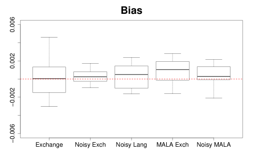
Figure 1: Boxplot of the bias estimate of $\theta$ for 20 datasets corresponding to the exchange, importance sampling exchange, Langevin and MALA algorithms.

Figure 1 shows the bias of the posterior means for each of the algorithms. We see that both the noisy exchange algorithm and the Langevin algorithm have a much smaller bias when compared to the two exchange algorithms. The two noisy algorithms perform better than the two exact algorithms. This is due to the improved mixing in the approximate algorithms, even though the true distribution is only approximately targeted. There is a trade off here between the bias and the efficiency. As the step size decreases, both the efficiency and bias decrease. The MALA-exchange appears better than the exchange, this is due to the informed proposal used in the MALA algorithm $\hat{\nabla}\log\pi(\theta|y)$. This informed proposal means the MALA-exchange will target areas of high probability in the posterior density, therefore increasing the chances of accepting a move at each iteration when compared to the standard exchange. Finally, in Figure 2 we display the estimated posterior density for each of the five algorithms together with the true posterior density for one of the $20$ datasets in the simulation study.

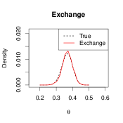
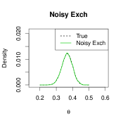
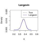
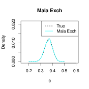
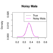
Figure 2: Estimated posterior densities corresponding to the exact and noisy algorithms corresponding to one of the datasets used in the Ising simulation study.

4.2 ERGM study

Here we explore how our algorithms may be applied to the exponential random graph model (ERGM) [2007] which is widely used in social network analysis. An ERGM is defined on a random adjacency matrix $Y$ of a graph on $n$ nodes (or actors) and a set of edges (dyadic relationships) $\{Y_{ij}:i=1,\dots,M;j=1,\dots,M\}$ where $Y_{ij}=1$ if the pair $(i,j)$ is connected by an edge, and $Y_{ij}=0$ otherwise. An edge connecting a node to itself is not permitted so $Y_{ii}=0$. The dyadic variables maybe be undirected, whereby $Y_{ij}=Y_{ji}$ for each pair $(i,j)$, or directed, whereby a directed edge from node $i$ to node $j$ is not necessarily reciprocated.

The likelihood of an observed network $y$ is modelled in terms of a collection of sufficient statistics $\{s_{1}(y),\dots,s_{m}(y)\}$, each with corresponding parameter vector $\theta=\{\theta_{1},\dots,\theta_{m}\}$,

$$f(y|\theta)=\dfrac{q_{\theta}(y)}{Z(\theta)}=\frac{\exp\left\{\sum_{l=1}^{m}\theta_{l}s_{l}(y)\right\}}{Z(\theta)}.$$

For example, typical statistics include $s_{1}(y)=\sum_{i<j}y_{ij}$ and $s_{2}(y)=\sum_{i<j<k}y_{ik}y_{jk}$ which are, respectively, the observed number of edges and two-stars, that is, the number of configurations of pairs of edges which share a common node. It is also possible to consider statistics which count the number of triangle configurations, that is, the number of configurations in which nodes $i,j,k$ are all connected to each other.

4.2.1 The Florentine Business dataset

Here, we consider a simple 16 node undirected graph: the Florentine family business graph. This concerns the business relations between some Florentine families in around 1430. The network is displayed in Figure 3. We propose to estimate the following 2-dimensional model.

$$f(y|\theta)=\frac{1}{Z(\theta)}\exp\left(\theta_{1}s_{1}(y)+\theta_{2}s_{2}(y)\right),$$

where $s_{1}(y)$ is the number of edges in the graph and $s_{2}(y)$ is the number of two-stars.

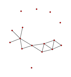
Figure 3: Florentine family business.

Before we could run the algorithms, certain parameters had to be tuned. We used a flat prior $N(0,100)$ in all of the algorithms. The Langevin, MALA exchange and noisy MALA exchange algorithms all depend on a stepsize matrix $\Sigma$. This matrix determines the scale of proposal values for each of the parameters. This matrix should be set up so that proposed values for $\theta$ accommodate the different scales of the posterior density of $\theta$. In order to have good mixing in the algorithms we chose a $\Sigma$ which relates to the shape of the posterior density. Our approach was to aim to relate $\Sigma$ to the covariance of the posterior density. To do this, we equated $\Sigma$ to an estimate of the inverse of the second derivative of the log posterior at the maximum a posteriori estimate $\theta^{*}$. As the true value of the MAP is unknown, we used a Robbins-Monro algorithm [1951] to estimate this. The Robbins-Monro algorithm takes steps in the direction of the slope of the distribution. It is very similar to Algorithm 8 except without the added noise and follows the stochastic process

$$\theta_{n+1}=\theta_{n}+\epsilon_{n}\widehat{\nabla}^{y_{\theta_{n}}}\log\pi(\theta_{n}|y),$$

$$\mbox{where }\sum^{N}_{i=0}\epsilon_{n}<\infty\;\mbox{and}\;\sum^{N}_{i=0}\epsilon^{2}_{n}<\infty.$$

The values of $\epsilon$ decrease over time and once the difference between successive values of this process is less than a specified tolerance level, the algorithm is deemed to have converged to the MAP. The second derivative of the log posterior is derived by differentiating (7) yielding

$$\nabla^{2}\log\pi(\theta^{*}|y)=\mathrm{Cov}_{y^{*}|\theta^{*}}(s(y^{*}))+\nabla^{2}\log\pi(\theta^{*})$$ (9)

In turn, $\mathrm{Cov}_{y^{*}|\theta^{*}}(s(y^{*}))$ from (9) can be estimated using Monte Carlo based on draws from the likelihood $f(y|\theta^{*})$. We used the inverse of the estimate of the second derivative of the log posterior as an estimate for the curvature of our log posterior distribution. The matrix $\Sigma$ we used was this estimate of the curvature multiplied by a scalar. We multiply by a scalar to achieve different acceptance rates for the algorithms. This is similar to choosing a variance for the proposal in a standard Metropolis-Hastings algorithm. If too small a value is chosen for the scalar, the algorithm will propose small steps and take a long time to fully explore the posterior distribution. If too large a value is chosen for the scalar, the chain will inefficiently explore the target distribution. A number of pilot runs were made to find a value for the scalar which gave the desired acceptance rates for each of the algorithms. The MALA exchange and Noisy MALA exchange algorithms were tuned to have an acceptance rate of approximately $25\%$ and a similar $\Sigma$ matrix was used in the noisy Langevin algorithm. If the second derivative matrix is singular, a problem can arise, in that is impossible to calculate the inverse of the matrix. Further information on singular matrices can be found in numerical linear algebra literature, such as [1996].

The algorithms were time normalised, each using 30 seconds of CPU time. An extra $N=50$ graphs were simulated for the noisy exchange, noisy Langevin, MALA exchange and noisy MALA exchange algorithms. The auxiliary step to draw $y^{\prime}$ was run for 1000 iterations followed by an extra 200 iterations thinned by a factor of 4 yielding $N=50$ graphs. To compare the results to a “ground truth”, the BERGM algorithm of [2011] was run for an large number of iterations equating to 2 hours of CPU time. This algorithm involves a population MCMC algorithm and uses the current state of the population to help make informed proposals for the chains within the population.

Table 1 shows the posterior means and standard deviations for the various algorithms. Figures 4 and 5 shows the chains, densities and autocorrelation plots. In Table 1 we see that the noisy exchange algorithm had improved mean estimates when compared to the exchange algorithm. The MALA exchange and Noisy MALA exchange algorithms both had better mean estimates than the noisy Langevin algorithm, although in all cases the posterior standard deviation was underestimated.

The ACF plots in Figures 4 and 5 show how all of the noisy algorithms displayed better mixing when compared to the exchange algorithm. The density plots show that all of the algorithms with the exception of the noisy Langevin estimated the mode of the true density well but they underestimated the standard deviation.

The noisy Langevin performed poorly. A problem of Langevin diffusion as pointed out in [2011] is that convergence to the invariant distribution is no longer guaranteed for finite step size owing to the first-order integration error that is introduced. This discrepancy is corrected by the Metropolis step in the MALA exchange and noisy MALA exchange but not in the Langevin algorithm. Since our Noisy Langevin algorithm approximates Langevin diffusion we are approximating an approximation. There are two levels of approximations which leaves more room for error.

	Edge		2-star
Method	Mean	SD	Mean	SD
BERGM	-2.675	0.647	0.188	0.155
Exchange	-2.573	0.568	0.146	0.133
Noisy Exchange	-2.686	0.526	0.167	0.122
Noisy Langevin	-2.281	0.513	0.081	0.119
MALA Exchange	-2.518	0.62	0.136	0.128
Noisy MALA	-2.584	0.498	0.144	0.113

Table 1: Posterior means and standard deviations.

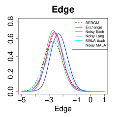
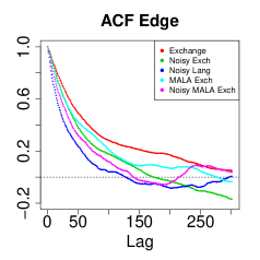
Figure 4: Chains, density plot and ACF plot for the edge statistic.

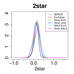
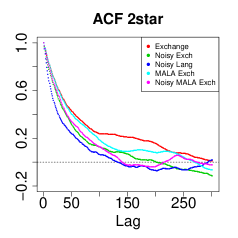
Figure 5: Chains, density plot and ACF plot for the 2-star statistic.

4.2.2 The Molecule dataset

The Molecule dataset is a 20 node graph, shown in Figure 6. We consider a four parameter model which includes the number of edges in the graph, the number of two-stars, the number of three-stars and the number of triangles.

$$f(y|\theta)=\frac{1}{Z(\theta)}\exp\left(\theta_{1}s_{1}(y)+\theta_{2}s_{2}(y)+\theta_{3}s_{3}(y)+\theta_{4}s_{4}(y)\right)$$

The $\Sigma$ parameter was chosen in a similar fashion to the Florentine business example. The Robbins-Monro algorithm was run for 20,000 iterations to find an estimate of the MAP, 4,000 graphs were then simulated at the estimated MAP and these were used to calculate an estimate of the second derivative using Equation (9). The matrix $\Sigma$ was the inverse of this estimate was calculated multiplied by a scalar. The scalar was chosen as a value which achieved the desired acceptance rate, a number of pilot runs were used to get a reasonable value for the scalar. This was carried out for both the MALA exchange and noisy MALA exchange and a similar $\Sigma$ matrix was used for the noisy Langevin algorithm. The ERGM model for the molecule data is more challenging than the model for the Florentine data due to the extra two parameters.

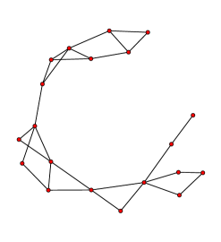
Figure 6: Molecule network

The BERGM algorithm of [2011] was again used as a “ground truth”. This algorithm was run for a large number of iterations equating to 4 hours of CPU time. This gave us accurate estimates against which to compare the various algorithms. The five algorithms were each run for 100 seconds of CPU time. Table 2 shows the posterior mean and standard deviations of each of the four parameters for each of the algorithms. The results for the Molecule dataset model are similar to the Florentine business dataset model. In Table 2 we see that the noisy exchange algorithm improved on the standard exchange algorithm. The MALA exchange improved on noisy Langevin and the Noisy MALA improved on the MALA exchange.

Figure 7 and Figure 8 show the densities and the autocorrelation plots of the algorithms. The autocorrelation plots show that the noisy algorithms had less correlation than the exchange algorithm. The densities show that again the algorithms, when run on the Molecule model, performed in the same manner as the Florentine model. The algorithms with the exception of the noisy Langevin algorithm estimated the mode well but underestimated the standard deviation. The noisy Langevin algorithm did not estimate the mean or standard deviations well.

	Edge		2-star		3-Star		Triangle
Method	Mean	SD	Mean	SD	Mean	SD	Mean	SD
BERGM	2.647	2.754	-1.069	0.953	-0.021	0.483	1.787	0.646
Exchange	1.889	2.142	-0.797	0.744	-0.138	0.385	1.593	0.519
Noisy Exch	1.927	2.444	-0.757	0.823	-0.176	0.422	1.543	0.53
Noisy Lang	1.679	3.65	-0.509	1.429	-0.466	0.787	1.633	0.573
MALA Exch	2.391	2.095	-0.938	0.795	-0.113	0.451	1.454	0.598
Noisy MALA Exch	2.731	2.749	-1.054	0.886	-0.041	0.417	1.519	0.492

Table 2: Posterior means and standard deviations.

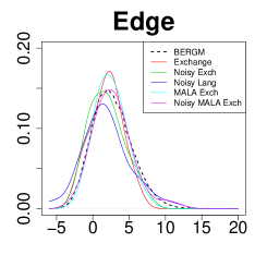
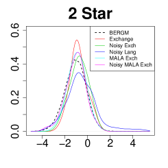
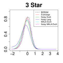
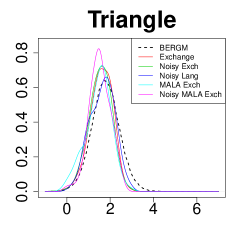
Figure 7: Density plots of the 4 parameters for the molecule example.

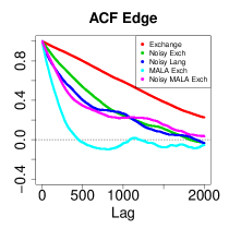
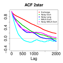
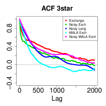
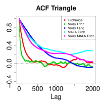
Figure 8: ACF plots for the 4 parameters for the molecule example.

5 Conclusion

The results in this paper give bounds on the total variation between a Markov chain with the desired target distribution, and the Markov chain of a noisy MCMC algorithm. An important question for future work concerns the statistical efficiency of estimators given by ergodic averages of the chain output. This is a key question since the use of noisy MCMC will usually be motivated by the inefficiency of a standard alternative algorithm. This inefficiency may be: statistical, where the standard algorithm is only capable of exploring the parameter space slowly (as can be the case for the standard exchange algorithm); or, computational, where a single iteration of the standard algorithm is too computationally expensive for the method to be practically useful (as is the case for large data sets, examined by Korattikara et al. (?)). If we introduce a noisy MCMC algorithm to overcome the inefficiency, usually the rationale is that the combined statistical and computational efficiency is sufficiently improved to outweigh the effect of any bias that is introduced. To study this theoretically we need to investigate the asymptotic variance of estimators from noisy MCMC algorithms. Andrieu and Vihola (?) have examined this question for pseudo-marginal algorithms of the GIMH type, and have shown the asymptotic variance for pseudo-marginal algorithms is always larger than for the corresponding “ideal” algorithm. One might expect a similar result to hold for noisy MCMC algorithms, in which case the effect of this additional variance on top of the aforementioned bias should be a consideration when employing noisy MCMC.

A further area for future work lies in relaxing the requirement for the ideal non-noisy chain to be uniformly ergodic. This property does not hold in many cases: the results in this paper are intended as the first steps towards future work that would obtain results that hold more generally.

Acknowledgements

The Insight Centre for Data Analytics is supported by Science Foundation Ireland under Grant Number SFI/12/RC/2289. Nial Friel’s research was also supported by an Science Foundation Ireland grant: 12/IP/1424.

Appendix A Proofs

Proof of Corollary 2.3. We apply Theorem 2.1. First, note that we have

$$P(\theta,{\rm d}\theta^{\prime})=\delta_{\theta}({\rm d}\theta^{\prime})\left[1-\int{\rm d}th(t|\theta)\min\left(1,\alpha(\theta,t)\right)\right]+h(\theta^{\prime}|\theta)\min\left(1,\alpha(\theta,\theta^{\prime})\right)$$

and

$$\hat{P}(\theta,{\rm d}\theta^{\prime})=\delta_{\theta}({\rm d}\theta^{\prime})\left[1-\iint{\rm d}t{\rm d}y^{\prime}h(t|\theta)F_{t}(y^{\prime})\min\left(1,\hat{\alpha}(\theta,t,y^{\prime})\right)\right]\\ +\int{\rm d}y^{\prime}F_{\theta^{\prime}}(y^{\prime})\Bigl{[}h(\theta^{\prime}|\theta)\min\left(1,\hat{\alpha}(\theta,\theta^{\prime},y^{\prime})\right)\Bigr{]}.$$

So we can write

$$(P-\hat{P})(\theta,{\rm d}\theta^{\prime})\\ =\delta_{\theta}({\rm d}\theta^{\prime})\iint{\rm d}t{\rm d}y^{\prime}h(t|\theta)F_{t}(y^{\prime})\Bigl{[}\min\left(1,\hat{\alpha}(\theta,t,y^{\prime})\right)-\min\left(1,\alpha(\theta,t)\right)\Bigr{]}\\ +\int{\rm d}y^{\prime}F_{\theta^{\prime}}(y^{\prime})\Bigl{[}h(\theta^{\prime}|\theta)\min\left(1,\alpha(\theta,\theta^{\prime})\right)-h(\theta^{\prime}|\theta)\min\left(1,\hat{\alpha}(\theta,\theta^{\prime},y^{\prime})\right)\Bigr{]}$$

and, finally,

$$\|P-\hat{P}\|=\frac{1}{2}\sup_{\theta}\int|P-\hat{P}|(\theta,{\rm d}\theta^{\prime})\\ =\frac{1}{2}\sup_{\theta}\Biggl{\{}\Biggl{|}\iint{\rm d}t{\rm d}y^{\prime}h(t|\theta)F_{t}(y^{\prime})\Bigl{[}\min\left(1,\hat{\alpha}(\theta,t,y^{\prime})\right)-\min\left(1,\alpha(\theta,t)\right)\Bigr{]}\Biggr{|}\\ +\Biggl{|}\iint{\rm d}y^{\prime}{\rm d}\theta^{\prime}F_{\theta^{\prime}}(y^{\prime})\left[h(\theta^{\prime}|\theta)\min\left(1,\alpha(\theta,\theta^{\prime})\right)-h(\theta^{\prime}|\theta)\min\left(1,\hat{\alpha}(\theta,\theta^{\prime},y^{\prime})\right)\right]\Biggr{|}\Biggr{\}}\\ =\sup_{\theta}\Biggl{\{}\Biggl{|}\iint{\rm d}t{\rm d}y^{\prime}h(t|\theta)F_{t}(y^{\prime})\Bigl{[}\min\left(1,\hat{\alpha}(\theta,t,y^{\prime})\right)-\min\left(1,\alpha(\theta,t)\right)\Bigr{]}\Biggr{|}\Biggr{\}}\\ \leq\sup_{\theta}\iint{\rm d}y^{\prime}{\rm d}\theta^{\prime}F_{\theta^{\prime}}(y^{\prime})h(\theta^{\prime}|\theta)\Bigl{|}\min\left(1,\alpha(\theta,\theta^{\prime})\right)-\min\left(1,\hat{\alpha}(\theta,\theta^{\prime},y^{\prime})\right)\Bigr{|}\\ =\sup_{\theta}\int{\rm d}\theta^{\prime}h(\theta^{\prime}|\theta)\int{\rm d}y^{\prime}F_{\theta^{\prime}}(y^{\prime})\Bigl{|}\min(1,\alpha(\theta,\theta^{\prime}))-\min(1,\hat{\alpha}(\theta,\theta^{\prime},y^{\prime}))\Bigr{|}\\ \leq\sup_{\theta}\int{\rm d}\theta^{\prime}h(\theta^{\prime}|\theta)\delta(\theta,\theta^{\prime}).\quad\square$$

Proof of Lemma 2.4. We still use Theorem 2.1, note that

$$\|P_{\Sigma}-\hat{P}_{\Sigma}\|=\frac{1}{2}\sup_{\theta}\int\Biggl{|}\frac{1}{\sqrt{2\pi|\Sigma|}}\exp\left[-\frac{\|\Sigma^{-\frac{1}{2}}(\theta^{\prime}-\theta-\frac{\Sigma}{2}\nabla\log\pi(\theta))\|^{2}}{2}\right]\\ -\frac{1}{\sqrt{2\pi|\Sigma|}}\exp\left[-\frac{\|\Sigma^{-\frac{1}{2}}(\theta^{\prime}-\theta-\frac{\Sigma}{2}\hat{\nabla}^{y^{\prime}}\log\pi(\theta))\|^{2}}{2}\right]\Biggr{|}{\rm d}\theta^{\prime}F_{\theta}({\rm d}y^{\prime})\\ =\frac{1}{2}\sup_{\theta}\iint\frac{1}{\sqrt{2\pi}}\exp\left[-\frac{\|t\|^{2}}{2}\right]\Biggl{|}1\\ -\exp\left[\frac{\|t\|^{2}}{2}-\frac{\|t+\frac{\Sigma^{\frac{1}{2}}}{2}(\nabla\log\pi(\theta)-\hat{\nabla}^{y^{\prime}}\log\pi(\theta))\|^{2}}{2}\right]\Biggr{|}{\rm d}tF_{\theta}({\rm d}y^{\prime})\\ =\frac{1}{2}\sup_{\theta}\iint\frac{1}{\sqrt{2\pi}}\exp\left[-\frac{\|t\|^{2}}{2}\right]\Biggl{|}1-\exp\Biggl{[}\frac{t^{T}\Sigma^{\frac{1}{2}}(\nabla\log\pi(\theta)-\hat{\nabla}^{y^{\prime}}\log\pi(\theta))}{2}\\ -\frac{1}{8}\|\Sigma^{\frac{1}{2}}(\nabla\log\pi(\theta)-\hat{\nabla}^{y^{\prime}}\log\pi(\theta))\|^{2}\Biggr{]}\Biggr{|}{\rm d}tF_{\theta}({\rm d}y^{\prime}).$$

Now, note that

$$\int\frac{1}{\sqrt{2\pi}}\exp\left[-\frac{\|t\|^{2}}{2}\right]\Biggl{|}1\\ -\exp\left[\frac{t^{T}\Sigma^{\frac{1}{2}}(\nabla\log\pi(\theta)-\hat{\nabla}^{y^{\prime}}\log\pi(\theta))}{2}-\frac{1}{8}\|\Sigma^{\frac{1}{2}}(\nabla\log\pi(\theta)-\hat{\nabla}^{y^{\prime}}\log\pi(\theta))\|^{2}\right]\Biggr{|}{\rm d}t\\ =\mathbb{E}\Biggl{|}1-\exp\left(a^{T}X-\frac{\|a\|^{2}}{2}\right)\Biggr{|}$$

where $X\sim\mathcal{N}(0,I)$ and $a=\Sigma^{\frac{1}{2}}[\nabla\log\pi(\theta)-\hat{\nabla}^{y^{\prime}}\log\pi(\theta)]/2$. Then:

$$\mathbb{E}\Biggl{|}1-\exp\left(a^{T}X-\frac{\|a\|^{2}}{2}\right)\Biggr{|} =\exp\left(-\frac{\|a\|^{2}}{2}\right)\mathbb{E}\Biggl{|}\exp\left(a^{T}X\right)-\exp\left(\frac{\|a\|^{2}}{2}\right)\Biggr{|}$$

$$=\exp\left(-\frac{\|a\|^{2}}{2}\right)\mathbb{E}\Biggl{|}\exp\left(a^{T}X\right)-\mathbb{E}\left[\exp\left(a^{T}X\right)\right]\Biggr{|}$$

$$\leq\exp\left(-\frac{\|a\|^{2}}{2}\right)\sqrt{{\rm Var}[\exp\left(a^{T}X\right)]}$$

$$=\exp\left(-\frac{\|a\|^{2}}{2}\right)\sqrt{\mathbb{E}\left[\exp\left(2a^{T}X\right)\right]-\mathbb{E}\left[\exp\left(a^{T}X\right)\right]^{2}}$$

$$=\exp\left(-\frac{\|a\|^{2}}{2}\right)\sqrt{\exp(2\|a\|^{2})-\exp(\|a\|^{2})}$$

$$=\sqrt{\exp(\|a\|^{2})-1}.$$

So finally,

$$\|P_{\Sigma}-\hat{P}_{\Sigma}\|\leq\frac{1}{2}\sup_{\theta}\int F_{\theta}({\rm d}y^{\prime})\sqrt{\exp\left[\frac{\|\Sigma^{\frac{1}{2}}(\nabla\log\pi(\theta)-\hat{\nabla}^{y^{\prime}}\log\pi(\theta))\|^{2}}{4}\right]-1}\\ \leq\frac{1}{2}\sqrt{\sup_{\theta}\int F_{\theta}({\rm d}y^{\prime})\exp\left[\frac{\|\Sigma^{\frac{1}{2}}(\nabla\log\pi(\theta)-\hat{\nabla}^{y^{\prime}}\log\pi(\theta))\|^{2}}{4}\right]-1}\leq\sqrt{\delta}.\quad\square$$

Proof of Lemma 3.1. We only have to check that

$$\mathbb{E}_{y^{\prime}\sim F_{\theta^{\prime}}}\left|\hat{\alpha}(\theta,\theta^{\prime},y^{\prime})-\alpha(\theta,\theta^{\prime})\right|\\ \leq\int{\rm d}y^{\prime}f(y^{\prime}|\theta^{\prime})\Bigl{|}\alpha(\theta,\theta^{\prime})-\hat{\alpha}(\theta,\theta^{\prime},y^{\prime})\Bigr{|}\\ =\frac{h(\theta|\theta^{\prime})\pi(\theta^{\prime})q_{\theta^{\prime}}(y)}{h(\theta^{\prime}|\theta)\pi(\theta)q_{\theta}(y)}\mathbb{E}_{y_{1}^{\prime},\dots,y_{N}^{\prime}\sim f(\cdot|\theta^{\prime})}\left|\frac{1}{N}\sum_{i=1}^{N}\frac{q_{\theta}(y_{i}^{\prime})}{q_{\theta^{\prime}}(y_{i}^{\prime})}-\frac{Z(\theta)}{Z(\theta^{\prime})}\right|\\ \leq\frac{1}{\sqrt{N}}\frac{h(\theta|\theta^{\prime})\pi(\theta^{\prime})q_{\theta^{\prime}}(y)}{h(\theta^{\prime}|\theta)\pi(\theta)q_{\theta}(y)}\sqrt{{\rm Var}_{y_{1}^{\prime}\sim f(y_{1}^{\prime}|\theta^{\prime})}\left(\frac{q_{\theta_{n}}(y_{1}^{\prime})}{q_{\theta^{\prime}}(y_{1}^{\prime})}\right)}.\quad\square$$

Proof of Theorem 3.2. Under the assumptions of Theorem 3.2, note that (4) leads to

$$\alpha(\theta_{n},\theta^{\prime})=\frac{\pi(\theta^{\prime})q_{\theta^{\prime}}(y)Z(\theta_{n})}{\pi(\theta_{n})q_{\theta_{n}}(y)Z(\theta^{\prime})}\frac{h(\theta_{n}|\theta^{\prime})}{h(\theta^{\prime}|\theta_{n})}\geq\frac{1}{c_{\pi}^{2}c_{h}^{2}\mathcal{K}^{4}}.$$ (10)

Let us consider any measurable subset $B$ of $\Theta$ and $\theta\in\Theta$. We have

$$P(\theta,B) =\int_{B}\delta_{\theta}({\rm d}\theta^{\prime})\left[1-\int{\rm d}th(t|\theta)\min\left(1,\alpha(\theta,t)\right)\right]$$

$$\hskip 56.9055pt+\int_{B}{\rm d}\theta^{\prime}h(\theta^{\prime}|\theta)\min\left(1,\alpha(\theta,\theta^{\prime})\right)$$

$$\geq\int_{B}{\rm d}\theta^{\prime}h(\theta^{\prime}|\theta)\min\left(1,\alpha(\theta,\theta^{\prime})\right)$$

$$\geq\frac{1}{c_{\pi}^{2}c_{h}^{2}\mathcal{K}^{4}}\int_{B}{\rm d}\theta^{\prime}h(\theta^{\prime}|\theta)\text{ thanks to~{}\eqref{proofstep1}}$$

$$\geq\frac{1}{c_{\pi}^{2}c_{h}^{3}\mathcal{K}^{4}}\int_{B}{\rm d}\theta^{\prime}.$$

This proves that $\Theta$ is a small set for the Lebesgue measure (multiplied by constant $1/c_{\pi}^{2}c_{h}^{3}\mathcal{K}^{4}$) on $\Theta$. According to Theorem 16.0.2 page 394 in Meyn and Tweedie [1993], this proves that:

$$\sup_{\theta}\|\delta_{\theta}P-\pi(\cdot|y)\|\leq C\rho^{n}$$

where

$$C=2\text{ and }\rho=1-\frac{1}{c_{\pi}^{3}c_{h}^{3}\mathcal{K}^{4}}$$

(note that, by definition, $\mathcal{K},c_{\pi},c_{h}>1$ so we necessarily have $0<\rho<1$). So, Condition (H1) in Lemma 2.3 is satisfied.

Moreover,

$$\delta(\theta,\theta^{\prime}) =\frac{h(\theta|\theta^{\prime})\pi(\theta^{\prime})q_{\theta^{\prime}}(y)}{h(\theta^{\prime}|\theta)\pi(\theta)q_{\theta}(y)}\sqrt{{\rm Var}_{y^{\prime}\sim f(y^{\prime}|\theta^{\prime})}\left(\frac{q_{\theta_{n}}(y^{\prime})}{q_{\theta^{\prime}}(y^{\prime})}\right)}$$

$$\leq c_{h}^{2}c_{\pi}^{2}\frac{q_{\theta^{\prime}}(y)}{q_{\theta}(y)}\sqrt{\mathbb{E}_{y^{\prime}\sim f(y^{\prime}|\theta^{\prime})}\left[\left(\frac{q_{\theta_{n}}(y^{\prime})}{q_{\theta^{\prime}}(y^{\prime})}\right)^{2}\right]}\leq c_{h}^{2}c_{\pi}^{2}\mathcal{K}^{4}.$$

So, Condition (H2) in Lemma 2.3 is satisfied. We can apply this lemma and to give

$$\sup_{\theta_{0}\in\Theta}\|\delta_{\theta_{0}}P^{n}-\delta_{\theta_{0}}\hat{P}^{n}\|\leq\frac{\mathcal{C}}{\sqrt{N}}$$

with

$$\mathcal{C}=c_{\pi}^{2}c_{h}^{2}\mathcal{K}^{4}\left(\lambda+\frac{C\rho^{\lambda}}{1-\rho}\right)$$

with $\lambda=\left\lceil\frac{\log(1/C)}{\log(\rho)}\right\rceil$. $\square$

Proof of Lemma 3.3. Note that

$$\nabla\log\pi(\theta)-\hat{\nabla}^{x^{\prime}}=\frac{1}{N}\sum_{i=1}^{N}s(y^{\prime}_{i})-\mathbb{E}_{y^{\prime}\sim f_{\theta}}[s(y^{\prime})].$$

So we have to find an upper bound, uniformly over $\theta$, for

$$D:=\mathbb{E}_{y^{\prime}\sim F_{\theta_{n}}}\left\{\exp\left[\frac{\sigma^{2}}{2}\left\|\Sigma^{\frac{1}{2}}\left(\frac{1}{N}\sum_{i=1}^{N}s(y^{\prime}_{i})-\mathbb{E}_{y^{\prime}\sim f_{\theta}}[s(y^{\prime})]\right)\right\|^{2}\right]-1\right\}.$$

Let us put $V:=\frac{1}{N}\sum_{i=1}^{N}V^{(i)}:=\frac{1}{N}\sum_{i=1}^{N}\Sigma^{\frac{1}{2}}\{s(y^{\prime}_{i})-\mathbb{E}_{y^{\prime}\sim f_{\theta}}[s(y^{\prime})]\}$ and denote $V_{j}$ ($j=1,\dots,k$) the coordinates of $V$, and $V_{j}^{(i)}$ ($j=1,\dots,k$) the coordinates of $V^{(i)}$. We have

$$D =\mathbb{E}\left\{\exp\left[\frac{1}{2}\sum_{j=1}^{k}V_{j}^{2}\right]-1\right\}$$

$$=\mathbb{E}\left\{\exp\left[\frac{1}{k}\sum_{j=1}^{k}\frac{k}{2}V_{j}^{2}\right]-1\right\}$$

$$\leq\frac{1}{k}\sum_{j=1}^{k}\mathbb{E}\left\{\exp\left[\frac{k}{2}V_{j}^{2}\right]-1\right\}.$$

Now, remark that $V_{j}=\frac{1}{N}\sum_{i=1}^{n}V_{j}^{(i)}$ with $-\mathcal{S}\|\Sigma\|\leq V_{j}^{i}\leq\mathcal{S}\|\Sigma\|$ so, Hoeffding’s inequality ensures, for any $t\geq 0$,

$$\mathbb{P}\left(\left|\sqrt{N}V_{j}\right|\geq t\right)\leq 2\exp\left[-\frac{t^{2}}{2\mathcal{S}^{2}\|\Sigma\|^{2}}.\right]$$

As a consequence, for any $\tau>0$,

$$\mathbb{E}\exp\left[\frac{k}{2}V_{j}^{2}\right] =\mathbb{E}\exp\left[\frac{k}{2N}\left(\sqrt{N}V_{j}\right)^{2}\right]$$

$$=\mathbb{E}\exp\left[\frac{k}{2N}\left(\sqrt{N}V_{j}\right)^{2}\mathbf{1}_{|\sqrt{N}V_{j}|\leq\tau}\right]$$

$$\quad\quad+\mathbb{E}\exp\left[\frac{k}{2N}\left(\sqrt{N}V_{j}\right)^{2}\mathbf{1}_{|\sqrt{N}V_{j}|>\tau}\right]$$

$$=\exp\left(\frac{k\tau^{2}}{2N}\right)+\int_{\tau}^{\infty}\exp\left(\frac{k}{2N}x^{2}\right)\mathbb{P}\left(\left|\sqrt{N}V_{j}\right|\geq x\right){\rm d}x$$

$$\leq\exp\left(\frac{k\tau^{2}}{2N}\right)+2\int_{\tau}^{\infty}\exp\left[\left(\frac{k}{2N}-\frac{1}{2\mathcal{S}^{2}\|\Sigma\|^{2}}\right)x^{2}\right]{\rm d}x$$

$$=\exp\left(\frac{k\tau^{2}}{2N}\right)+2\sqrt{\frac{2\pi}{\frac{1}{\mathcal{S}^{2}\|\Sigma\|^{2}}-\frac{2k}{N}}}\mathbb{P}\left(|\mathcal{N}|>\tau\sqrt{\frac{1}{\frac{1}{\mathcal{S}^{2}\|\Sigma\|^{2}}-\frac{2k\sigma^{2}}{N}}}\right)$$

$$\leq\exp\left(\frac{k\tau^{2}}{2N}\right)+2\sqrt{\frac{2\pi}{\frac{1}{\mathcal{S}^{2}\|\Sigma\|^{2}}-\frac{2k}{N}}}\exp\left[-\frac{\tau^{2}}{\left(\frac{2}{\mathcal{S}^{2}\|\Sigma\|^{2}}-\frac{4k}{N}\right)}\right]$$

$$\leq\exp\left(\frac{k\tau^{2}}{2N}\right)+2\sqrt{\frac{2\pi}{\frac{1}{\mathcal{S}^{2}\|\Sigma\|^{2}}-\frac{2k}{N}}}\exp\left[-\frac{\tau^{2}\mathcal{S}^{2}\|\Sigma\|^{2}}{2}\right]$$

where $\mathcal{N}\sim\mathcal{N}(0,1)$. Now, we assume that $N>4k\mathcal{S}^{2}\|\Sigma\|^{2}$. This leads to $\frac{1}{\mathcal{S}^{2}\|\Sigma\|^{2}}-\frac{2k}{N}>\frac{1}{2\mathcal{S}^{2}\|\Sigma\|^{2}}$. This simplifies the bound to

$$\mathbb{E}\exp\left[\frac{k}{2}V_{j}^{2}\right]\leq\exp\left(\frac{k\tau^{2}}{2N}\right)+4\sqrt{\pi}\mathcal{S}\|\Sigma\|\exp\left[-\frac{\tau^{2}\mathcal{S}^{2}\|\Sigma\|^{2}}{2}\right].$$

Finally, we put $\tau=\sqrt{\log(N/k)/(2\mathcal{S}^{2}\|\Sigma\|^{2})}$ to get

$$\mathbb{E}\exp\left[\frac{k}{2}V_{j}^{2}\right]\leq\exp\left(\frac{k\log\left(\frac{N}{k}\right)}{4\mathcal{S}^{2}\|\Sigma\|^{2}N}\right)+\frac{4k\sqrt{\pi}\mathcal{S}\|\Sigma\|}{N}.$$

It follows that

$$D\leq\exp\left(\frac{k\log(N)}{4\mathcal{S}^{2}\|\Sigma\|^{2}N}\right)-1+\frac{4k\sqrt{\pi}\mathcal{S}\|\Sigma\|}{N}.$$

This ends the proof. $\square$

Proof of Lemma 3.4. We just check all the conditions of Theorem 2.2. First, from Lemma 3.3, we know that $\|P_{\Sigma}-\hat{P}_{\Sigma}|\leq\sqrt{\delta/2}\rightarrow 0$ when $N\rightarrow\infty$. Then, we have to find the function $V$. Note that here:

$$\nabla\log\pi(\theta|y) =\nabla\log\pi(\theta)+s(y)-\mathbb{E}_{y|\theta}[s(y)]$$

$$=-\frac{\theta}{s^{2}}+s(y)-\mathbb{E}_{y|\theta}[s(y)]$$

$$\asymp-\frac{\theta}{s^{2}}.$$

Then, according to Theorem 3.1 page 352 in [1996a] (and its proof), we know that for $\Sigma<s^{2}$, for some positive numbers $a$ and $b$, for $V(\theta)=a\theta$ when $\theta\geq 0$ and $V(\theta)=-b\theta$ for $\theta<0$, there is a $0<\delta<1$, $\beta>0$ and an inverval $I$ with

$$\int V(\theta)P_{\Sigma}(\theta_{0},{\rm d}\theta)\leq\delta V(\theta_{0})+L\mathbf{1}_{I}(\theta_{0}),$$

and so $P_{\Sigma}$ is geometrically ergodic with function $V$. We calculate

$$\int V(\theta)\hat{P}_{\Sigma}(\theta_{0},{\rm d}\theta) =\mathbb{E}_{y^{\prime}}\left[\frac{1}{\sqrt{2\pi\Sigma}}\int_{\mathbb{R}}V(\theta)\exp\left(-\frac{\left(\theta-\theta_{0}-\frac{\Sigma}{2}\hat{\nabla}^{y^{\prime}}\log\pi(\theta_{0}|y)\right)}{2\Sigma}\right){\rm d}\theta\right]$$

$$=\mathbb{E}_{y^{\prime}}\Biggl{[}\frac{1}{\sqrt{2\pi\Sigma}}\int_{\mathbb{R}}V\left[\theta+\frac{\Sigma}{2}(\hat{\nabla}^{y^{\prime}}\log\pi(\theta_{0}|y)-\nabla\log\pi(\theta_{0}|y))\right]$$

$$\quad\quad\exp\left(-\frac{\left(\theta-\theta_{0}-\frac{\Sigma}{2}\nabla\log\pi(\theta_{0}|y)\right)}{2\Sigma}\right){\rm d}\theta\Biggr{]}$$

$$=\frac{1}{\sqrt{2\pi\Sigma}}\int_{\mathbb{R}}\mathbb{E}_{y^{\prime}}\left\{V\left[\theta+\frac{\Sigma}{2}(\hat{\nabla}^{y^{\prime}}\log\pi(\theta_{0}|y)-\nabla\log\pi(\theta_{0}|y))\right]-V(\theta)\right\}$$

$$\quad\quad\exp\left(-\frac{\left(\theta-\theta_{0}-\frac{\Sigma}{2}\nabla\log\pi(\theta_{0}|y)\right)}{2\Sigma}\right){\rm d}\theta+\int V(\theta)P_{\Sigma}(\theta_{0},{\rm d}\theta)$$

and:

$$\mathbb{E}_{y^{\prime}}\left\{V\left[\theta+\frac{\Sigma}{2}(\hat{\nabla}^{y^{\prime}}\log\pi(\theta_{0}|y)-\nabla\log\pi(\theta_{0}|y))\right]-V(\theta)\right\}$$

$$\leq\max(a,b)\mathbb{E}_{y^{\prime}}\left|\frac{1}{N}\sum_{i=1}^{N}\{\mathbb{E}[s(y_{i}^{\prime})]-s(y_{i}^{\prime})\}\right|$$

$$\leq 2\mathcal{S}\max(a,b).$$

So,

$$\int V(\theta)\hat{P}_{\Sigma}(\theta_{0},{\rm d}\theta) \leq\int V(\theta)P_{\Sigma}(\theta_{0},{\rm d}\theta)+2\mathcal{S}\max(a,b)$$

$$\leq\delta V(\theta_{0})+[L+2\mathcal{S}\max(a,b)].$$

So all the assumptions of Theorem 2.2 are satisfied, and we can conclude that $\|\pi_{\Sigma}-\pi_{\Sigma,N}\|\xrightarrow[N\rightarrow\infty]{}0$. $\square$

References

- 2012 Ahn, S., A. Korattikara and M. Welling (2012), Bayesian Posterior Sampling via Stochastic Gradient Fisher Scoring. In Proceedings of the 29th International Conference on Machine Learning
- 2009 Andrieu, C. and G. Roberts (2009), The pseudo-marginal approach for efficient Monte-Carlo computations. The Annals of Statistics 37(2), 697–725
- 2012 Andrieu, C. and M. Vihola (2012), Convergence properties of pseudo-marginal Markov chain Monte Carlo algorithms. Preprint arXiv:1210.1484
- 2014 Bardenet, R., A. Doucet and C. Holmes (2014), Towards scaling up Markov chain Monte Carlo: an adaptive subsampling approach. In Proceedings of the 31st International Conference on Machine Learning
- 2003 Beaumont, M. A. (2003), Estimation of population growth or decline in genetically monitored populations. Genetics 164, 1139–1160
- 1974 Besag, J. E. (1974), Spatial Interaction and the Statistical Analysis of Lattice Systems. Journal of the Royal Statistical Society, Series B 36, 192–236
- 2011 Bottou, L. and O. Bousquet (2011), The tradeoffs of large-scale learning. In S. Sra, S. Nowozin and S. J. Wright (eds.), Optimization for machine learning, pp. 351–368, MIT Press
- 2011 Bühlmann, P. and S. Van de Geer (2011), Statistics for high-dimensional data. Springer
- 2011 Caimo, A. and N. Friel (2011), Bayesian inference for exponential random graph models. Social Networks 33, 41–55
- 2012 Dalalyan, A. and A. B. Tsybakov (2012), Sparse regression learning by aggregation and Langevin. J. Comput. System Sci. 78(5), 1423–1443
- 2013 Ferré, D., L. Hervé and J. Ledoux (2013), Regular perturbation of -geometrically ergodic Markov chains. Journal of applied probability 50(1), 184–194
- 2004 Friel, N. and A. N. Pettitt (2004), Likelihood estimation and inference for the autologistic model. Journal of Compuational and Graphical Statistics 13, 232–246
- 2009 Friel, N., A. N. Pettitt, R. Reeves and E. Wit (2009), Bayesian inference in hidden Markov random fields for binary data defined on large lattices. Journal of Computational and Graphical Statistics 18, 243–261
- 2007 Friel, N. and H. Rue (2007), Recursive computing and simulation-free inference for general factorizable models. Biometrika 94, 661–672
- 1984 Geman, S. and D. Geman (1984), Stochastic relaxation, Gibbs distributions, and the Bayesian restoration of images. IEEE Transactions on Pattern Analysis and Machine Intelligence 6, 721–741
- 1994 Gilks, W., G. Roberts and E. George (1994), Adaptive direction sampling. The Statistician 43, 179–189
- 2011 Girolami, M. and B. Calderhead (2011), Riemann manifold Langevin and Hamiltoian Monte Carlo methods (with discussion). Journal of the Royal Statistical Society, Series B 73, 123–214
- 1996 Golub, G. and C. V. Loan (1996), Matrix computations. Johns Hopkins University Press, Baltimore, MD
- 1996 Kartashov, N. V. (1996), Strong Stable Markov Chains. VSP, Utrecht
- 2014 Korattikara, A., Y. Chen and M. Welling (2014), Austerity in MCMC Land: Cutting the Metropolis-Hastings Budget. In Proceedings of the 31st International Conference on Machine Learning, pp. 681–688
- 2011 Liang, F. and I.-H. Jin (2011), An Auxiliary Variables Metropolis-Hastings Algorithm for Sampling from Distributions with Intractable Normalizing Constants. Technical report
- 2012 Marin, J.-M., P. Pudlo, C. P. Robert and R. J. Ryder (2012), Approximate Bayesian computational methods. Statistics and Computing 22(6), 1167–1180
- 1993 Meyn, S. and R. L. Tweedie (1993), Markov Chains and Stochastic Stability. Cambridge University Press
- 2005 Mitrophanov, A. Y. (2005), Sensitivity and convergence of uniformly ergodic Markov chains. Journal of Applied Probability 42, 1003–1014
- 2006 Moller, J., A. Pettit, R. Reeves and K. Bertheksen (2006), An efficient Markov chain Monte Carlo method for distributions with intractable normalising constants. Biometrika 93, 451–458
- 2006 Murray, I., Z. Ghahramani and D. MacKay (2006), MCMC for doubly-intractable distributions. In Proceedings of the 22nd Annual Conference on Uncertainty in Artificial Intelligence UAI06, Arlington, Virginia, AUAI Press
- 2012 Nicholls, G. K., C. Fox and A. Muir Watt (2012), Coupled MCMC with a randomized acceptance probability. Preprint arXiv:1205.6857
- 1996 Propp, J. and D. Wilson (1996), Exactly sampling with coupled Markov chains and applications to statistical mechanics. Random Structures and Algorithms 9, 223–252
- 2004 Reeves, R. and A. N. Pettitt (2004), Efficient recursions for general factorisable models. Biometrika 91, 751–757
- 1951 Robbins, H. and S. Monro (1951), A Stochastic Approximation Method. The Annals of Mathematical Statistics 22(3), 400–407
- 2002 Roberts, G. O. and O. Stramer (2002), Langevin Diffusions and Metropolis-Hastings Algorithms. Methodology and Computing in Applied Probability 4, 337–357
- 1996a Roberts, G. O. and R. L. Tweedie (1996a), Exponential Convergence of Langevin Distributions and their Discrete Approximations. Bernoulli 2(4), 341–363
- 1996b Roberts, G. O. and R. L. Tweedie (1996b), Geometric Convergence and Central Limit Theorems for Multidimensional Hastings and Metropolis Algorithm. Biometrika 83(1), 95–110
- 2007 Robins, G., P. Pattison, Y. Kalish and D. Lusher (2007), An introduction to exponential random graph models for social networks. Social Networks 29(2), 169–348
- 1996 Tibshirani, R. (1996), Regression Shrinkage and Selection via the Lasso. Journal of the Royal Statistical Society B 58(1), 267–288
- 1984 Valiant, L. (1984), A theory of the learnable. Communications of the ACM 27(11), 1134–1142
- 2011 Welling, M. and Y. W. Teh (2011), Bayesian Learning via Stochastic Gradient Langevin Dynamics. In Proceedings of the 28th International Conference on Machine Learning, pp. 681–688