Limitless Regression Discontinuity

Abstract

Conventionally, regression discontinuity analysis contrasts a univariate regression’s limits as its independent variable, $R$, approaches a cut-point, $c$, from either side. Alternative methods target the average treatment effect in a small region around $c$, at the cost of an assumption that treatment assignment, $\mathcal{I}\left[R<c\right]$, is ignorable vis a vis potential outcomes.

Instead, the method presented in this paper assumes Residual Ignorability, ignorability of treatment assignment vis a vis detrended potential outcomes. Detrending is effected not with ordinary least squares but with MM-estimation, following a distinct phase of sample decontamination. The method’s inferences acknowledge uncertainty in both of these adjustments, despite its applicability whether $R$ is discrete or continuous; it is uniquely robust to leading validity threats facing regression discontinuity designs.

1 Introduction

In a regression discontinuity design (RDD; Thistlethwaite  Campbell, 1960), treatment is allocated to subjects for whom a “running variable” $R$ exceeds (or falls below) a pre-determined cut-point. Lee (2008) has argued that the regression discontinuity design features “local randomization” of treatment assignment, and is therefore “a highly credible and transparent way of estimating program effects” (Lee  Lemieux, 2010 , p. 282).

Take the RDD found in Lindo, Sanders  Oreopoulos (2010 ; hereafter LSO). LSO attempt to estimate the effect of “academic probation,” an intervention for struggling college students, on students’ subsequent grade point averages (GPAs). At one large Canadian university, students with first-year GPAs below a cutoff were put on probation. Comparing subsequent GPA ($Y$) for students with first-year GPA ($R$) just below and above the cutoff should reveal the effectiveness of the policy at promoting satisfactory grades.

LSO’s data analysis, like that of most RDD studies, used ordinary regression analyses to target an extraordinary parameter. In Imbens and Lemieux’s (2008) telling, for example, the target of estimation is not the average treatment effect (ATE) in any one region around the cutoff but rather the “local” average treatment effect, or “LATE”: the limit of ATEs over concentric ever-shrinking regions, essentially an ATE over an infinitesimal interval. Following this “limit understanding,” it is common to analyze RDDs using regression to estimate the functional relationships of $r$ to $\mathbb{E}(Y|R=r)$ on either side of the cutoff. The difference between the two regression functions, as evaluated at the cut-point, is interpreted as the treatment effect (e.g., Berk  Rauma, 1983; Angrist  Lavy, 1999).

However, the GPAs in the academic probation study are discrete, measured in 1/100s of a grade point; hence, limits of functions of GPA do not exist. Further, re-analysis of LSO’s RDD uncovers evidence of “social corruption” (Wong  Wing, 2016)—some students appear to have finely manipulated their GPAs to avoid probation. This necessitates excluding subjects immediately on or around the cut-point—precisely those students to whom the LATE might most plausibly pertain. Either circumstance calls into question the appropriateness of limit-based methods.

Cattaneo . (2015) base RDD inference on the model that, in effect, the RDD is a randomized controlled trial (RCT), at least in sufficiently small neighborhoods of the cut-point. Under this assumption, once attention is confined to such a region, the difference of $Y$-means between subjects falling above and below the cut-point estimates the ATE within that region. Despite being natural as a specification of Lee’s local randomization concept, the RCT model involves an independence condition that is rarely plausible in RDDs. In the LSO example, the data refute this model—unless one rejects all but the small share of the sample contained in a narrow band of the cutpoint, sacrificing power and external validity.

To circumvent limitations of the simple RCT model, and of the limit understanding, this paper weds parametric and local randomization ideas into a novel identifying assumption termed “residual ignorability.” The residual ignorability assumption and corresponding ATE estimates pertain to all subjects in the data analysis sample; discrete GPAs do not pose a threat. Manipulation of the running variable remains a threat, but one that Section 3’s combination of sample pruning and robust M-estimation is uniquely equipped to address.

The remainder of Section 1 uses a public health example to introduce residual ignorability and to review distribution-free analysis of RCTs. Limitless RDD analysis combines these ideas with classical, wholly parametric methods for RDDs (§ 2.1), and RDD specification tests (§ 2.2). Section 3 adapts residual ignorability to data configurations typical of education studies, and sets out an analysis plan anticipating common challenges of RDD analysis. Section 4 executes the plan with the LSO study, Section 5 explores the method’s performance in simulations, and Section 6 takes stock. Replication materials, including R code, are available as a GitHub repository, https://github.com/adamSales/lrd.

1.1 The Death Toll from Hurricane Maria

Hurricane Maria struck the island of Puerto Rico on September 20, 2017. In spite of widespread devastation, for nearly a year official statistics pegged the number of hurricane-induced deaths at just 64. Estimates from investigative journalists and academic researchers were higher. Santos-Lozada and Howard’s (2018) authoritative analysis considered recorded mortality in months before and after the hurricane, estimating Maria to have caused 1,139 deaths in excess of those that would have occurred otherwise. This section demonstrates the concept of residual ignorability, if not the scope and particulars of the method detailed in Section 3, in a reanalysis of these monthly death counts.

In this example, let $i=1,\dots,12$ denote the months of 2017 and let Puerto Rico’s monthly death counts constitute the outcome, $Y_{i}$. The running variable $R_{i}=i$ is month order and months are “treated,” $Z_{i}=1$, if and only if $R\geq 9$, Hurricane Maria having occurred in September. Following Neyman (1923) and Rubin (1974), we may then take each $i$ to have two potential outcomes: $Y_{Ti}$, a potential response under the treatment condition (the number of deaths that would occur were $i$ to fall after Maria); and $Y_{Ci}$, a potential response to control (the death count were $i$ to fall before Maria). For each $i$, at most one of $Y_{Ci}$ and $Y_{Ti}$ is observed, depending on $Z_{i}$; observed responses $Y$ coincide with $ZY_{T}+(1-Z)Y_{C}$. Differences $\tau_{i}=Y_{Ti}-Y_{Ci}$, $i=9,\ldots,12$, represent mortality caused by Maria. We will discuss RDD estimation of total excess mortality for 2017, $\sum_{i\geq 9}\tau_{i}$, in due course.The remainder of this section demonstrates how to test the hypothesis $\tau_{i}\equiv 0$, all $i$, using a Fisher randomization test—but without assuming the following independence property:

• $$Y_{C}\perp Z.$$ (1)

Although RCTs validate (1) as a matter of course, the assumption is implausibly strong for the mortality series surrounding Maria. For (1) to hold, $Z$ must be independent of monthly death counts that would have been observed in the absence of exposure to Maria: the distribution underlying the September through December counts must be no different than that of the year’s first eight months. Monthly mortality in Puerto Rico for the period 2010–2017, shown in the left panel of Figure 1, shows there is no precedent for such an equivalence. Rather, a marked seasonal trend is apparent, with death counts being higher in the winter months than during the rest of the year; (1) cannot be sustained. (For RDD methodology nonetheless founded on (1), see Cattaneo . (2015) or Mattei  Mealli (2016).)

Dependence between $R$ and $Y_{C}$, violating (1), is common in RDDs; when present, it must be addressed. Inspection of the 2010–16 mortality series (Figure 1) reveals a periodic, non-linear relationship between calendar month and death count, with some years appearing to be more hazardous than others. To accommodate these factors, we regressed 2010–2016 monthly death counts on dummy variables for year and a periodic b-spline for month order, with knots at February, May, August, and November. There are several outlying observations, one of which Santos-Lozada  Howard (2018) remove from the sample prior to analysis. Rather than identifying and removing outliers informally, we fit the regression model using a robust redescending M-estimator, which systematically down-weights and sometimes rejects outliers that would otherwise be influential (Maronna ., 2006). This model fit is displayed as a dashed black line in Figure 1.

Now let $\hat{Y}_{C}(R_{i})$ be that model’s prediction for month $i$ in 2017, and let $e(Y_{i}|{R_{i}})=Y_{i}-\hat{Y}_{C}(R_{i})$ be the prediction residual, with potential values $e(Y_{Ci}|{R_{i}})=Y_{Ci}-\hat{Y}_{C}(R_{i})$ and $e(Y_{Ti}|{R_{i}})=Y_{Ti}-\hat{Y}_{C}(R_{i})$. Instead of (1), we assume only that the model we have fit to pre-2017 monthly death counts captured and removed seasonal mortality trends, such that the potential residuals $\{{E}_{Ci}:i\}\equiv\{e(Y_{Ci}|{R_{i}}):i\}$ can be regarded as random, at least as far as $Z$ is concerned:

$$E_{C}\perp Z.$$ (2)

The right panel of Figure 1 shows residualized death counts $E=e(Y|{R})$ as a function of month order $R$. Seasonal mean trends are no longer in evidence; (2) is thus more plausible than the standard ignorability assumption (1). Aside from a technical elaboration that will be necessary to apply our method in the general case (§ 3.1), assumption (2) is residual ignorability, this paper’s alternative to Strong Ignorability as a basis for analysis of RDDs.

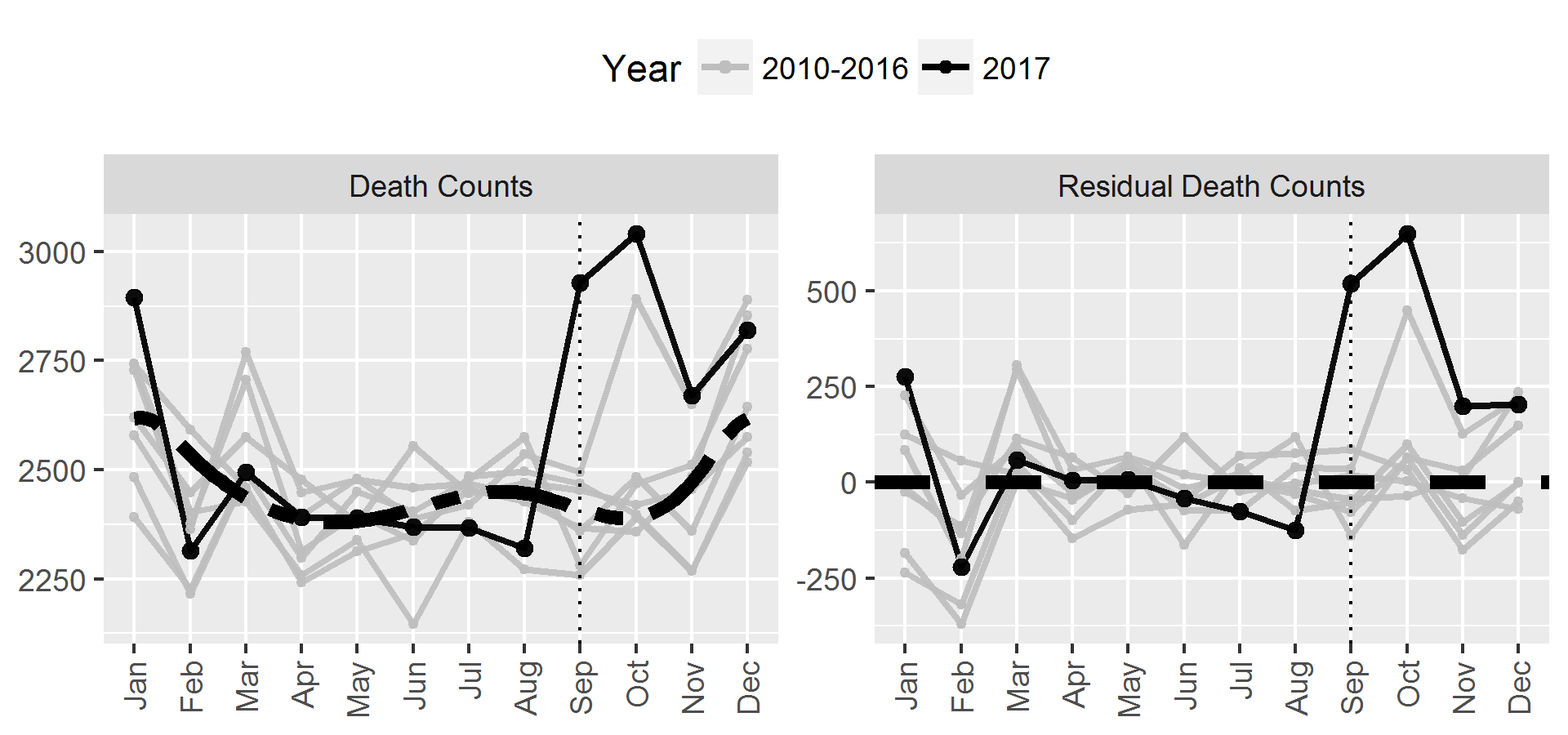
Figure 1: Monthly death counts in Puerto Rico from years 2010–2017, before and after residualization. The plot on the left shows monthly death counts, adjusted for month length. A vertical dotted line denotes September, the month Maria hit. The fit of the robust model described in the text is shown as a dashed black line. The plot on the right shows the monthly residuals of the model fit, with a dashed line denoting zero.

1.2 Using (2) to Test the Hypothesis of Strictly No Effect

In parallel with Fisherian analysis of RCTs (Fisher, 1935), which can be regarded as conditioning on the potential outcome random vector $\bm{Y}_{C}\equiv\{Y_{Ci}:i\}$, our Maria analysis conditions on the potential residual vector $\bm{E}_{C}\equiv\{E_{Ci}\}_{i=1}^{12}$. (Here and throughout, boldface indicates the concatenation of $n$ variables or constants.) The approach applies to the testing of “strict” null hypotheses, hypotheses that designate a value for each $E_{Ti}-E_{Ci}$ with $Z_{i}=1$, not just $\mathbb{E}(E_{T}-E_{C}|Z=1)$. This includes the hypothesis of strictly no effect, $H_{0}:Y_{T}\equiv Y_{C}$, under which $\bm{E}_{T}\equiv\bm{E}_{C}=\bm{E}$.

In this analysis $Y$, $R$, and $Z$ data for years 2010–2016 are treated as fixed—formally, inference will be made after conditioning not only on $\bm{E}_{C}$ but also on the values of $\{(Y_{i},R_{i},Z_{i}):i\leq 0\}$. To make use of Fisher’s (1935) permutation technique, we likewise condition on the realized sizes $N_{1}$ and $N_{0}$ of the treatment and control group samples, where $N_{j}\equiv\sum_{i=1}^{12}\mathcal{I}\left[Z_{i}=j\right]$. Such conditioning is appropriate because the conditioning statistic $\bm{A}^{*}=\{\bm{E}_{C},N_{1},N_{0};(Y_{-71},R_{-71}),\ldots,(Y_{-1},R_{-1})\}$ is ancillary to, i.e. carries no information about, the target of estimation $\mathbb{E}(E_{T}-E_{C})$.

Under $H_{0}$, we may exactly enumerate the sampling distribution of any test statistic $t(\bm{E}_{C},\bm{Z})=t(\bm{E},\bm{Z})$ conditional on $\bm{A}^{*}$; the permutational p-value is found by comparing a test statistic to its conditional distribution thus enumerated. In this analysis $\hat{Y}_{C}(R_{i})$ cannot itself be influenced by Maria, since it is based on a model fit to pre-Maria death counts (cf. Sales ., 2018). Hence, the effect of Maria on $E$ (i.e. $E_{T}-E_{C}$) is exactly equal to its effect on $Y$. The null hypothesis $H_{0}$ states that Hurricane Maria caused precisely no change to each month’s death count, nor to its residual. Under $H_{0}$, we condition on $\bm{A}^{*}$ and calculate the sampling distribution of the treatment group residual mean $t(\bm{e},\bm{Z})=\bar{e}_{Z=1}$, by calculating its value for all $\binom{N_{0}+N_{1}}{N_{1}}=\binom{12}{4}=495$ possible permutations of $\bm{Z}$. The null distribution of $t(\bm{e},\bm{Z})$ is simply that of the mean of a size-4, without-replacement sample from $\{e_{1},\ldots,e_{12}\}$. It turns out that only 2 permutations of $\bm{Z}$ result in test statistic values higher than the realized value $\bar{e}_{z=1}=$1,569 (which is unique in the distribution). This implies a two-sided “mid” p-value (Agresti  Gottard, 2005) of $2(2+0.5)/495\approx 0.01$ for $H_{0}$.

This combination of regression and permutation testing applies just as readily to test the hypothesis $E_{T}=E_{C}+c$, for any constant $c$. In the Maria example, no such hypothesis is sustainable at level 0.05 unless $c\geq$ 170, corresponding to 680 excess deaths due to the hurricane. Upper confidence limits and Hodges-Lehmann-type estimates of the effect can also be obtained in this way. Rather that pursuing this approach further, we now turn to developing a residual ignorability-based procedure using M-estimation (Huber, 1964; Stefanski  Boos, 2002 ; also called “generalized estimating equations” or “generalized method of moments”), which is better adapted to data scenarios without the luxury of a separate sample for estimation of trends in the absence of treatment.

2 Review of Selected RDD Methods

The method presented in this paper builds on existing methods for RDDs. This section selectively reviews relevant literature.

Let $Z\in\{0,1\}$ indicate assignment to treatment ($Z=1$) as opposed to control ($Z=0$). For the remainder of the paper, let $R$ be the centered running variable—the difference between the running variable and the RDD threshold $c$—so that $Z\equiv\mathcal{I}\left[R<0\right]$, $\mathcal{I}\left[R\leq 0\right]$, $\mathcal{I}\left[R\geq 0\right]$ or $\mathcal{I}\left[R>0\right]$, depending on how intervention eligibility relates to the threshold, where $\mathcal{I}\left[x\right]=1$ if $x$ is true and $0$ otherwise. Let $Y$ represent the outcome of interest. For simplicity assume non-interference, the model that a subject’s response may depend on his but not also on other subjects’ treatment assignments (Cox, 1958; Rubin, 1978). Thus we may take each $i$ to have two potential outcomes, $y_{Ti}$ and $y_{Ci}$, at most one of which is observed; observed responses $Y$ coincide with $ZY_{T}+(1-Z)Y_{C}$.

2.1 The ANCOVA Model for RDDs

The classical analysis of covariance (ancova) model for groups $i=1,\ldots,k$, each including subjects $j=1,\ldots,n_{i}$, says that $Y_{ij}=\alpha_{i}+\beta X_{ij}+\epsilon_{ij}$, where $\epsilon_{ij}\sim\mathrm{Normal}(0,\sigma^{2})$ is independent of the continuous covariate $X_{ij}$. In the classical development of RDDs, ancova with $k=2$ groups—treated and untreated—is a leading option among statistical models (Thistlethwaite  Campbell, 1960). A potential outcomes version of the model is $Y_{Ci}=\alpha_{0}+\beta R_{i}+\epsilon_{Ci}$ and $Y_{Ti}=\alpha_{1}+\beta R_{i}+\epsilon_{Ti}$, with $\epsilon_{Ci}\sim\mathrm{Normal}(0,\sigma^{2})$ and $\epsilon_{Ti}\sim\mathrm{Normal}(0,\sigma^{2})$. In marked contrast to RCTs, it is not required that $(Y_{T},Y_{C})\perp Z$: to the contrary, both $Y_{C}$ and $Y_{T}$ are presumed to associate with $R$, which in turn determines $Z$. Nonetheless, under this model the estimated $Z$ coefficient from the model

$$Y_{i}=\alpha+\beta R_{i}+\tau Z_{i}+\epsilon_{i},$$ (3)

fit using ordinary least squares (OLS), is unbiased for $\alpha_{1}-\alpha_{0}$. Under the ancova model, this estimation target coincides with $\lim_{r\downarrow 0}\mathbb{E}(Y|R=r)-\lim_{r\uparrow 0}\mathbb{E}(Y|R=r)$ and, simultaneously, limit-free estimation targets such as $\mathbb{E}Y_{T}-\mathbb{E}Y_{C}$.

The OLS approach estimates $\tau$ as a parameter in regression model (3). In contrast, the analysis of § 1.2 took place in two separate steps: first, adjust outcomes for $R$; then, test hypotheses by contrasting adjusted outcomes of treated and untreated subjects. OLS and the ancova model can be also be used for hypothesis testing, with steps paralleling those of § 1.2; this brings an important advantage to be described in § 2.1.1. Consider the hypothesis $H:Y_{T}=Y_{C}+\tau$. Define ${{Y}_{H}}={Y}-\tau{Z}$ (so that under $H$, $Y_{H}=Y_{C}$) and $e_{(a,b)}(\mathbf{y}_{H}|{\mathbf{r}})={\mathbf{y}_{H}}-a-b\mathbf{r}$. Finally, test $H$ with statistic

$$d(\mathbf{Y}_{H},\mathbf{Z})=\overline{e_{(\hat{\alpha},\hat{\beta})}({{Y}_{H}}|{{R}})}_{Z=1}-\overline{e_{(\hat{\alpha},\hat{\beta})}({{Y}_{H}}|{{R}})}_{Z=0}$$ (4)

—where $\hat{\alpha}$ and $\hat{\beta}$ are estimated from an OLS fit of the variant of (3) with dependent variable $\mathbf{y}_{H}$. A more essential difference between the current section’s procedure and the permutational method of § 1.2 is that the null distribution of (4) is not tractable. (In § 1.2, test statistics’ permutation distributions were straightforwardly enumerable because slope and intercept parameters had been estimated from a separate sample; in (4), one cannot consider alternate realizations of $Z$ without also considering alternate realizations of $(\hat{\alpha},\hat{\beta})$.) However, under the parametric ancova model, with conditioning on $\mathbf{R}$ rather than on $(N_{0},N_{1},\mathbf{Y}_{C})$ as in § 1.2, $d(\mathbf{Y}_{H},\mathbf{Z})$ is straightforwardly Normal, with variance equal to the classical OLS variance of the coefficient on $Z$.

In general, the set {$c$: $H_{c}:Y_{T}=Y_{C}+c$ is not rejected at level $\alpha$}, which can be seen to be an interval, is a $100(1-\alpha)\%$ confidence interval for $\tau$ of the Rao score type (Agresti, 2011); the $c$ solving $d(\mathbf{y}_{H},\mathbf{z})=0$, which can be seen to be unique, is an M-estimate of $\tau$ under both the classical ancova model and various of its generalizations. In fact, the estimate for $\tau$ corresponding to these statistical tests is algebraically equal to the $Z$-coefficient from an OLS estimate of (3), and the two-sided 95% confidence interval induced in this manner is the familiar $\hat{\tau}\pm 1.96\,\mathrm{SE}(\tau)$. However, these equivalences do not necessarily extend to estimation strategies outside of OLS, such as the robust estimators of § 3.3 below.

2.1.1 Addressing the Wald interval’s shortcomings for fuzzy RDDs

RDDs susceptible to non-compliance—where subjects’ actual treatments may differ from $Z$—are called “fuzzy.” In these cases, let $D$ indicate whether treatment was actually received. This $D$ is an intermediate outcome, so there are corresponding potential outcomes $D_{C}$ and $D_{T}$, with $D\equiv ZD_{T}+(1-Z)D_{C}$. Subject $i$ is a non-complier if $D_{Ci}=1$ or $D_{Ti}=0$, though we will assume the monotonicity condition $D_{C}\equiv 0$; there may be subjects assigned to the treatment who avoid it, but no one gets treatment without being assigned to it. We shall also posit the exclusion restriction, that $Z$ influences $Y$ only by way of its effect on $D$ (Bloom, 1984; Angrist ., 1996; Imbens  Rosenbaum, 2005). Our focus of estimation is the “treatment-on-treated” effect (TOTE), $\mathbb{E}(Y_{T}-Y_{C}|D_{T}=1)$.

Statistical hypotheses about the TOTE take the form $H_{\tau}:Y_{T}=Y_{C}+D\tau$. To test $H_{\tau}$ under non-compliance, let $Y_{H}=Y-\tau D$, designate $t(\mathbf{y}_{H},\mathbf{r})$ as test statistic, and compare its value to a standard Normal distribution. (The only difference between hypothesis testing for a “strict” RDD, one with full compliance, versus a fuzzy RDD, is in the formulation of hypothesis $H$, and the construction of $Y_{H}$—the rest of the process remains unchanged [Rosenbaum, 1996].) When compliance is imperfect, this iterative method yields confidence intervals with better coverage than Wald-type confidence intervals—that is, intervals of form $\hat{\tau}\pm q_{*}\mathrm{SE}(\hat{\tau})$ with $\mathrm{SE}(\hat{\tau})$ a single, hypothesis-independent quantity (Imbens  Rosenbaum, 2005; Baiocchi ., 2014 , Sec. 7).

2.1.2 Robust Standard Error Estimation

The ancova model for $(Y_{T},Y_{C})$ is not readily dispensed with, but it may be relaxed. OLS estimates of $\alpha_{1}-\alpha_{0}$ and $\beta$ remain unbiased under non-Normality, provided the $\epsilon$s have expectation 0 and bounded variances. The ordinary ancova standard error does not require Normality of the $(\epsilon_{i}:i)$, either, for use in large samples, although it does require that they have a common variance. To test $\mathbb{E}\{e_{\hat{\theta}}({Y_{H}}|{R})|Z=1\}=\mathbb{E}\{e_{\hat{\theta}}({Y_{H}}|{R})|Z=0\}$ under potential heteroskedasticity, one estimates $\mathrm{Var}\left\{d(\mathbf{Y}_{H},\mathbf{Z})\right\}$ using a sandwich or Huber-White estimator, $\mathrm{SE}_{s}^{2}\left\{d(\mathbf{Y}_{H},\mathbf{Z})\right\}$ (Huber, 1967; MacKinnon  White, 1985; Long  Ervin, 2000; Bell  McCaffrey, 2002; Pustejovsky  Tipton, 2017), and refers $d(\mathbf{Y}_{H},\mathbf{Z})/\mathrm{SE}_{s}$ to a $t$ or standard Normal reference distribution. Sandwich standard errors confer robustness to misspecification of $\mathrm{Var}(e_{\hat{\theta}}(Y_{H}|{R})\mid R)$, not of $\mathbb{E}(Y_{H}|R)$ (Freedman, 2006), the latter being the topic of the following section.

2.2 Threats to RDD Validity and some Remedies

The ancova model for RDDs encodes additional assumptions, beyond normality and homoskedasticity of regression errors and full compliance with treatment assignment, which are not so easily dispensed with. Methodological RDD literature has responded with specification tests to detect these threats, or with flexible estimators that seek to avoid them.

2.2.1 Covariate Balance Tests

Analysis of RCTs and quasiexperiments often hinges on assumptions of independence of $\mathbf{Z}$ from $(\mathbf{X},\mathbf{Y}_{C},\mathbf{Y}_{T})$. Although neither $\mathbf{Z}\perp\mathbf{Y}_{C}$ nor $\mathbf{Z}\perp\mathbf{Y}_{T}$ can be directly tested, since potential outcomes are only partly observed, assumptions of form $\mathbf{Z}\perp\mathbf{X}$ are falsifiable: researchers can conduct placebo tests for effects of $Z$ on $X$. Of course, treatment cannot affect pre-treatment variables; this is model-checking (Cox, 2006 , § 5.13).

Writing in the RDD context, Cattaneo . (2015) test for marginal associations of $\mathbf{Z}$ with covariates $\mathbf{X}_{i}$, $i=1,\ldots,k$, using the permutational methods that are applied in Fisherian analysis of RCTs (also see Li ., 2015). Relatedly, Lee  Lemieux (2010) recommend a test for conditional association, given $R$, of $\mathbf{Z}$ and $\mathbf{X}$, by fitting models like those discussed in § 2.1 for impact estimation, but with covariates rather than outcomes as independent variables. Viewing the $R$-slopes and intercepts as simultaneously estimated nuisance parameters, these are balance tests applied to the covariates’ residuals, rather than to the covariates themselves.

If there are multiple covariates there will be several such tests. To summarize their findings with a single p-value, the regressions themselves may be fused within a “seemingly unrelated regressions” model (Lee  Lemieux, 2010); however, to our knowledge, current software implementations do not support the combination of linear and generalized linear models, such as when covariates are of mixed type. Alternatives include hierarchical Bayesian modeling (Li ., 2015), or combining separate tests’ p-values using the Bonferroni principle or other multiple comparison corrections.

2.2.2 The McCrary Density Test

McCrary’s test for manipulation of treatment assignments (2008) can be understood as a placebo test with the density of $R$ as the independent variable. The test’s purpose is to expose the circumstance of subjects finely manipulating their $R$ values in order to secure or avoid assignment to treatment. Absent such a circumstance, if $R$ has a density then it should appear to be roughly the same just below and above the cutpoint. McCrary’s (2008) test statistic is the difference in logs of two estimates of $R$’s density at 0, based on observations with $R<0$ and $R>0$ respectively. Manipulation is expected to generate a clump just beside the cut point, on one side of it but not the other, and this in turn engenders imbalance in terms of distance from the cut-point.

2.2.3 Reducing the Bandwidth

In practice, specification test failures inform sample exclusions. When balance tests fail, Lee  Lemieux (2010) would select a bandwidth $b>0$, restrict analysis to observations with $R\in\mathcal{W}\subseteq[-b,b]$, and repeat the test on $\{i:r_{i}\in\mathcal{W}\}$. If that test fails, the process may be repeated with a new bandwidth $b^{\prime}<b$, and perhaps repeated again until arriving at suitable bandwidth. This may seem to call for a further layer of multiplicity correction, since any number of bandwidths may have been tested before identifying a suitable $b$; but it so happens that this form of sequential testing implicitly corrects for multiplicity, according to the sequential intersection union principle (SIUP; Rosenbaum, 2008 , Proposition 1; Hansen  Sales, 2015). Li . (2015) and Cattaneo . (2015) also suggest the use of covariate balance to select a bandwidth.

Restricting analysis to data within a bandwidth may change the interpretation of the result. The ATE and the TOTE refer to a discrete population, and reducing the bandwidth likewise reduces those populations—the new target populations consist of subjects for whom $|R|\leq b$. (In contrast, the definition of the LATE is unaffected by bandwidth choice.)

Failures of the density test are addressed by restricting estimation to observations with $|R|>a$, some $a\geq 0$ (e.g., Barreca ., 2011; Eggers ., 2015), and repeating the test. If this test rejects, we repeat the process with a new $a^{\prime}>a$, terminating the process when the p-value from the density test exceeds a pre-set threshold. By a second application of the SIUP, the size of this test sequence is equal to the size of each individual density test. Taken together, placebo and McCrary tests restrict the sample to $\mathcal{W}=(-b,b)$ or $(-b,-a)\cup(a,b)$.

2.2.4 Non-linear Models for Y as a function of R

The methods discussed in Sec 2.1 continue to apply if $\mathbb{E}(Y_{C}|R)=\alpha+R\beta$ is relaxed to $\mathbb{E}(Y_{C}|R)=\alpha+\bm{f}(R)\bm{\beta}$, for $\bm{f}(\cdot)$ a $1\times k$ vector valued function, and $\bm{\beta}$ a $k\times 1$ vector of coefficients. Unfortunately, if the model is fit by OLS, then such relaxation of assumptions can have the unwelcome side effect of undercutting the robustness of the analysis. The reasons have to do with mechanics of regression fitting.

Polynomial specifications $\mathbb{E}(Y|R=r)=\sum_{j=0}^{J}r^{j}\beta_{j}$ are common but often problematic; in combination with ordinary least squares fitting, they implicitly assign case weights that can vary widely and counterintuitively (Gelman  Imbens, 2018). This liability is already in evidence with $J=1$, the linear specification, where leverage increases with the square of $r-\bar{r}$. If analysts select a bandwidth $b$ that is slightly too large, then the analysis sample will include problematic observations near its outer boundaries, precisely where leverage is at its highest. If the analysis sample is contaminated near the cutpoint, the bad data may not threaten linear specifications, but with $J>1$ they can still bear undue leverage. In order to identify leverage points that are also influential, OLS fitting is sometimes combined with specialized diagnostics such as plots of Cook’s (1982) distances. Section 3.3 will discuss an alternate remedy.

3 Randomness and Regression in RDDs

The analysis of § 1.1 mounted an analogy between the Hurricane Maria RDD and a hypothetical RCT, but only after a preparatory step of modeling and removing the outcomes’ non-random component. In § 1.1, these two steps used two different datasets—we regressed $Y$ on $R$ using data from years prior to 2017, when Maria hit, and then used 2017 data to estimate effects, under the assumption of residual ignorability, (2). This luxury is unavailable in the typical RDD, in which both steps must use the same data, as in § 2.1. This section will describe a generalization of residual ignorability (2) to the typical case, along with robust analysis techniques incorporating the specification tests reviewed in § 2.2.

3.1 An Analytic Model for RDDs

This section will formalize residual ignorability for the typical RDD, which relies on a single dataset including variables $Y$, $R$, and $Z$. The assumption is that, after a suitable residual transformation, potential outcomes $Y_{C}$ are conditionally independent of $Z$. Hence, causal inference in an RDD may take the perspective that $Z$ is random due to randomness in $R$.

Suppose the statistician to have selected a detrending procedure: a trend fitter, i.e. a function of $\{({y}_{i},d_{i},r_{i})\}_{i=1}^{n}$ returning fitted parameters $\hat{\theta}$ in a sufficiently regular fashion, along with a family $\{e_{\theta}(\cdot|{\cdot}):\theta\}$ of residual or partial residual transformations, each mapping data $(\mathbf{y},\mathbf{r})$ to residuals $\{e_{\theta}(y_{i}|{{r}_{i}})\}_{i=1}^{n}$. Appendix A states the needed regularity condition, which is ordinarily met by OLS and always met with our preferred fitters (§ 3.3). Then, causal inference in an RDD proceeds from the following assumption:

• Given a detrending procedure $(\hat{\theta},e_{\theta}(y|{r}))$,

  $$e_{{\theta}_{0}}(Y_{C}|{R})\perp{Z}|\{R\in\mathcal{W}\}.$$ (5)

  Here $Z=f(R)$, for some deterministic $f$ (such as $f(r)=\mathcal{I}\left[r<0\right]$); ${\theta}_{0}$ is a constant such that $\sqrt{n}(\hat{\theta}-{\theta}_{0})$ is bounded in probability (and thus $\hat{\theta}\stackrel{{\scriptstyle P}}{{\rightarrow}}{\theta}_{0}$); $\mathcal{W}$ satisfies $\mathrm{Pr}(R\in\mathcal{W})>0$ and $0<\mathrm{Pr}(Z=1|R\in\mathcal{W})<1$.

Residual ignorability states that, though $Y_{C}$ may not be independent of $Z$, it admits a residual transformation bringing about such independence. With $e_{\hat{\theta}}(Y_{C}|{R})$ a suitable partial residual, residual ignorability is entailed by the ancova model (§ 2.1), or by the combination of any parametric model for $\mathbb{E}(Y_{C}|R)$ with a strict null $H$ relative to which the value of $Y_{C}$ can be reconstructed from the values of $Y$, $D$ and $Z$ (§ 1.2). (In either of these cases $e_{{\theta}_{0}}(Y_{C}|{R})$ is independent not only of $Z$ but also $R$, a modest strengthening of (5).)

Assuming residual ignorability, inference about treatment effects is made conditionally, on $\mathbf{A}=(e_{{\theta}_{0}}(\mathbf{Y}_{C}|{\mathbf{R}})$, $\mathbf{D}_{T},\{(Y_{Ti},Y_{Ci},D_{Ti},R_{i})\mathcal{I}\left[{R}_{i}\not\in\mathcal{W}\right]\}_{i=1}^{n})$. Conditioning on the full data vector when $R\not\in\mathcal{W}$ excludes observations for which (5) is not assumed. Conditioning on $e_{{\theta}_{0}}(\mathbf{Y}_{C}|{\mathbf{R}})$ removes little of the randomness in $\mathbf{R}$, leaving it available as a basis for inference. Uncoupled to $Y_{T}$’s, the detrended $Y_{C}$’s, $e_{{\theta}_{0}}(\mathbf{Y}_{C}|{\mathbf{R}})$, are in themselves uninformative about $\mathbb{E}(Y_{T}-Y_{C})$, so the variables comprising $\mathbf{A}$ are jointly ancillary, just as $\bm{A}^{*}$ was seen to be in Section 1.2. As in Fisher-style randomization inference for RCTs, some conditioning variables are unobserved; but this is not an impediment, at least for large-sample inferences.

Causal inference based on residual ignorability takes place in four steps: (1) choosing and validating the analysis sample or bandwidth, (2) choosing an appropriate fitting procedure (we recommend robust fitters), (3) treatment effect estimation and inference, and (4) post-fitting diagnostics. We will discuss each of these steps in sequence.

3.2 Pre-Fitting Diagnostics and Bandwidth Choice

If subject matter knowledge suggests that the ATE or TOTE would be most relevant for subjects with $|R|\leq b$, then $b$ might form an initial bandwidth choice. But it is also sensible to subject this choice to specification testing (§ 2.2).

Covariate balance or placebo tests for RDDs (§ 2.2.1) assess residual ignorability with a multivariate “outcome” $Y^{*}$ combining the actual outcome $Y$ with covariates $X$—(5) with $\mathbf{Y}_{C}^{*}=(\mathbf{X},{Y}_{C})$ in place of $Y_{C}$.

Of the placebo testing procedures discussed in § 2.2.1, that of Lee  Lemieux (2010) is best suited to this conception. In effect, it begins with preliminary detrending procedures—mechanisms to decompose $X$ into components that are systematic or unpredictable, vis a vis $\mathbf{R}$, just as ${\mathbf{Y}_{C}}$ will later be decomposed. Our analysis of the LSO data posits systematic components that are linear and logistic-linear in $R$, depending on whether $X$ is a measurement or binary variable. The placebo check adds $Z$ to the specification and tests whether its coefficient is zero. We implement these checks as Wald tests with heteroskedasticity-robust standard errors, as in § 2.1, using the Bonferroni method to combine placebo checks across covariates. To ensure adequate power to detect misspecification, we test at level $.15$, not $.05$.

We use sequential balance tests to adjust the bandwidth $b$, alongside McCrary density tests to further refine the analysis sample $\mathcal{W}$ (§ 2.2.3). These specification tests rely on covariates, $R$, and $Z$, but not on $Y$; therefore, selection of $\mathcal{W}$ is objectivity-preserving in the sense of Rubin (2007).

3.3 Robust Fitters

Observations in the analysis sample that do not satisfy residual ignorability can undercut the validity of an RDD analysis. Even moderate amounts of such contamination—specifically, contamination of a $O(n^{-1/2})$-sized share of the sample that happens to contain influential observations—can defeat OLS-based estimation strategies, rendering them inconsistent. Indeed, even some robust regression methods—those engineered to meet objectives other than bounding the influence function—may be misled (Stefanski, 1991). The inclusion of problematic observations in the analysis sample can be due to misspecification of the model for $\mathbb{E}(Y_{C}|R)$ (§ 2.2.4), manipulation of treatment assignments (§ 2.2.2), or other violations of residual ignorability, coupled with the failure of specification tests to detect these problems. However, no specification test is powerful enough to reliably detect moderate contamination; if the probability of a false alarm is controlled, then power to detect anomalies affecting only $O(n^{-1/2})$ of the sample can only tend to a number strictly less than 1. However $b$ and $\mathcal{W}$ are selected, at least some contamination may remain in the sample.

Accordingly, consistent estimation of ${\theta}_{0}$ requires robust M-estimators, in Yohai and Zamar’s (1997) sense, a class excluding maximum likelihood estimation while including modern MM-, SM-, and other estimators with bounded influence function (see also He, 1991 , Thm. 3). In MM-estimation as in OLS, coefficients $\bm{\beta}$ of a linear specification solve estimating equations $\sum_{i}\psi\left\{({y}_{i}-\bm{x}_{i}^{T}\bm{\beta})/s\right\}\bm{x}_{i}^{T}=\bm{0}$, where $s>0$ and $\psi(\cdot)$ is an odd function satisfying $\psi(0)=0$, $\psi^{\prime}(0)=1$, and $t\psi(t)\geq 0$; bounded influence fitters replace OLS’s $s\equiv 1$ with resistant preliminary estimates of residual scale and OLS’s $\psi(t)=t$ with a continuous $\psi$ that satisfies $\int_{0}^{\infty}\psi(t)dt<\infty$. This limits the loss incurred by the fitter for failing to adapt itself to a small portion of aberrant observations; it is permitted to systematically down-weight them instead.

The analyses and simulations presented below use MM-estimators with bisquare $\psi$ and “fast S” initialization (Salibian-Barrera  Yohai, 2006). We are not aware of prior work addressing potential contamination of an RDD sample with the assistance of bounded influence MM-estimation. Surprisingly, given their common origins in Huber (1964), MM-estimation is not routinely paired with sandwich estimates of variance, as in § 2.1.2 above. Exceptions include Stata’s mmregress and R’s lmrob, which optionally provide Huber-White standard errors (Verardi  Croux, 2009; Rousseeuw ., 2015); our analyses use the latter.

3.4 Treatment Effect Estimation and Inference

For inference about $\tau$ under the model $Y_{T}=Y_{C}+\tau D_{T}$, select a specification $\mu_{\beta}(\cdot)$ for $\mathbb{E}(Y_{C}|R)$ such as the linear model $\mu_{\beta}(R)=\alpha+R\beta$, a window of analysis $\mathcal{W}$, and a fitter.

Then, separately for each hypothesis $H:\tau=\tau_{0}$ under consideration, calculate $\mathbf{y}_{H}=\mathbf{y}-\mathbf{d}\tau_{0}$, and apply the chosen specification and fitter to $(\mathbf{y}_{H},\mathbf{r})$. The combination of the data, the model fit, and the residual transformation $e_{\theta}(\cdot|{\cdot})$ give rise to residuals $e_{\hat{\theta}}(\mathbf{y}_{H}|{\mathbf{r}})$, completing the detrending procedure. Whether $H$ is rejected or sustained is determined by the value of the sandwich-based ancova $t$-statistic in § 2.1.2.

In practice it is expedient to use a near-equivalent test by modifying the detrending procedure. When regressing $Y_{H}$ on $R$, include an additive contribution from $Z$, so that $\mu_{\theta}(R)=\alpha+R\beta$ is replaced with $\mu_{(\theta,\gamma)}(R)=\alpha+\beta R+\gamma Z$. With sandwich estimates of $\text{Cov}\{(\hat{\theta}_{H},\hat{\gamma}_{H})\}$, the $t$-ratio comparing $\hat{\gamma}_{H}$ to $\text{SE}_{s}(\hat{\gamma}_{H})$ induces a generalized score test (Boos, 1992). Implicitly it is a two-sample $t$-statistic with covariance adjustment for $R$ (with fitting via OLS, this correspondence would be exact, as noted in Section 2.1.2; with the robust MM-estimation we favor, the correspondence is one of large-sample equivalence; see Appendix A.2).

As in § 2.1, the corresponding M-estimate of the CACE is the value of $\tau_{0}$ making $\hat{\gamma}_{H}/\text{SE}_{s}(\hat{\gamma}_{H})$ equal 0; those $\tau_{0}$ for which $H:\tau=\tau_{0}$ is not rejected at level $\alpha$ constitute a $100(1-\alpha)\%$ confidence interval. Iteration is facilitated by regressing $\mathbf{y}$ on $\mathbf{r}$ and $\mathbf{z}$ with offset variable $\mathbf{d}\tau_{0}$; then only the offset needs to be modified to test $H:\tau=\tau_{1}$, $\tau_{1}\neq\tau_{0}$.

Strictly speaking, this estimation procedure relies on the assumption of a constant additive treatment effect, so that $Y_{T}=Y_{C}+D\tau_{0}$, for some constant $\tau_{0}$ (or, more generally, an exact model for treatment effects under which $Y_{C}$ could be recovered without error). This requirement is typical of estimators derived from the inversion of hypothesis tests (e.g. Imbens  Rosenbaum, 2005). However, due to its use of sandwich standard errors $\text{SE}_{s}(\cdot)$, our M-estimator is robust to some departures from this assumption. Specifically, under (5), $\hat{\tau}$ is consistent for $\tau_{0}$ solving

$$\mathbb{E}\big{\{}e_{{\theta}_{0}}(Y_{T}-D_{T}\tau_{0}|{R})\big{|}R\big{\}}\equiv\mathbb{E}\big{\{}e_{{\theta}_{0}}(Y_{C}|{R})\big{|}R\big{\}},$$

providing such a $\tau_{0}$ exists. That is, we assume the existence of a constant $\tau_{0}$ such that detrended $Y_{H}=Y-D\tau_{0}$ is equal to detrended $Y_{C}$ on average, if not exactly. The simulation study in § 5.1 bears out this robustness property.

3.5 Post-Fitting Diagnostics

Once the M-estimate for the treatment effect has been found, one inspects the corresponding regression fit for points of high influence. Robust MM-regression is helpful here. Besides making influential points easier to see in residual plots, it limits effects of data contamination, as non-conforming influence points are down-weighted as a result of the fitting process. This down-weighting is reflected in “robustness weights,” ranging from 1, for non-discounted observations, down to 0, for the most anomalous observations. Plotting robustness weights against residuals may expose opportunities to improve the fit of $\mu_{\theta}(R)$, or of the treatment effect model; plotting them against $R$ may expose contaminated sub-regions of $\mathcal{W}$ that specification testing failed to remove (Maronna ., 2006).

4 The Effect of Academic Probation

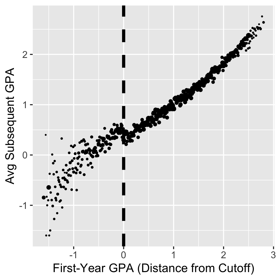
Figure 2: nextGPA by first-year GPA. Data are plotted with binning by unique value of first-year GPA, vertical coordinates being bin means of nextGPA and point sizes being proportional to bin size.

Figure (2) plots the LSO study’s primary outcome, GPA in the next term a student was enrolled following his first year (nextGPA), against first-year GPA. In all but 50 of 44,362 cases, being on academic probation (AP) coincided with whether first-year cumulative GPA—the running variable, $R$—fell below a cutoff. The university in question had three campuses, two having cutoffs of 1.5 and the other having a cutoff of 1.6. To combine data from the three schools, LSO centered each student’s first-year GPA at the appropriate $c$, making $r_{i}$ the difference of student $i$’s realized first-year GPA and the cutoff at his or her campus. Figure 2 follows LSO in this, displaying these $r_{i}$s on its $x$-axis; it also averages nextGPA values over students with equal first-year GPA, as opposed to plotting students individually. There is both a discontinuity in nextGPA values as $R$ crosses 0, and a distinctly non-null regression relationship on either side of that threshold. How large an AP effect may we infer from these features? How much of the data bear directly in this inference?

4.1 Choosing $\mathcal{W}$ and $\mu_{\theta}(\cdot)$

The region $\mathcal{W}_{0.5}=\pm$ 0.5 grade points includes students whose AP status could change if their grades in half their classes changed by a full mark (say from D to C). Simplicity recommends a linear specification for the outcome regression on the forcing variable, and the scatter of $Y$ versus $R$ did not suggest otherwise; so we designated $\mu_{\theta}(R_{i})=\alpha+\beta R_{i}$ and proceeded to specification checks, as discussed in Section 2.2.

Following LSO, we conducted placebo tests with high-school grade percentile rankings, number of credits attempted in first year of college, first language other than English, birth outside of North America, age at college entry, and which of the university’s 3 campuses the student attended. For the measurement variables, this amounted to fitting ancova models, whereas binary covariates were decomposed as logistic-linear in $R$ and $Z$; in both cases subsequent Wald tests of $Z$’s coefficient used Huber-White standard errors. For $\mathcal{W}_{0.5}$ each (Bonferroni-corrected) p-value exceeds $0.2$; downward adjustment of the bandwidth is not indicated.

The McCrary density test (McCrary, 2008) identifies a discontinuity in the running variable at the cut-point ($p<0.001$). AP is a dubious distinction, and savvy students may try to avoid it. Inspection of the distribution of $R$ reveals an unusual number of students whose first-year GPAs were exactly equal to the AP cutoff, $R=0$. It would be reasonable to suspect this significant McCrary finding of being an artifact of the discreteness of first-year GPAs, but Frandsen’s (2017) test for manipulation in a discrete running variable likewise detected an anomaly at a wide range of tuning parameter values: $p<0.001$ provided that $0\leq k\leq 0.1$. The finding is further corroborated by the fact that the number of students attempting four or fewer credits was also unusually high in the $R=0$ subgroup, suggesting that some students dropped courses to dodge AP. In any event, after removing the $R=0$ subgroup—that is, setting $\mathcal{W}=\{i:|R_{i}|\in(0,0.5)\}=\mathcal{W}_{0.5}\setminus\{i:R_{i}=0\}$—the McCrary procedure narrowly avoids rejecting the hypothesis of no manipulation ($p$ = 0.15).

4.2 AP Outcome Analysis

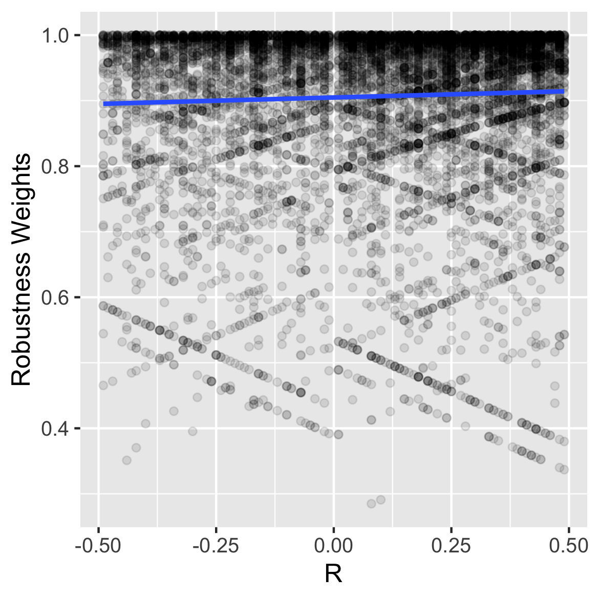
Figure 3: Robustness weights from robust MM-estimation of the model that $\mathbb{E}(Y_{C}|R=r)$ is linear in $r$ while $Y_{T}=Y_{C}+\tau_{0}D_{T}$, with $\tau_{0}$ set at $\hat{\tau}=$0.24.

Table 1 gives a set of estimates for the effect of AP, each obtained using the robust procedure of § 3.3–3.4. The first row of Table 1 gives our main result, with window of analysis $\mathcal{W}=\{i:|R_{i}|\in(0,0.5)\}$ and a linear model of $\mathbb{E}(Y_{C}|R)$, $\mu_{\theta}(R)=\alpha+\beta R$, estimating the TOTE based on subjects’ received treatments $D$. For the best fitting version of the model, robustness weights range from .28 to 1. These weights show little association with $R$, although the lowest weights occur just above the cut-point and near $\mathcal{W}$’s edges (Figure 3).

The main analysis estimates an average treatment effect of 0.24, with 95% confidence interval (0.17, 0.31).

Table 1’s next three rows relax each of the main model’s specifications. The row labeled “Adaptive $\mathcal{W}$” reports the results using the wider, adaptively chosen window $\mathcal{W}_{a}=\{i:|R_{i}|\in(0,$1.13$)\}$. The “Cubic” row allows for a cubic relationship between first-year GPA and subsequent GPA, with $\mu_{\theta}(R)=\alpha+\beta_{1}R+\beta_{2}R^{2}+\beta_{3}R^{3}$. This specification performed well in simulations (§ 5), suggesting that the warnings in Gelman  Imbens (2018) against higher-order global polynomials may not apply to analyses which use robust fitters. Finally, the “ITT” row gives an “intent to treat” analysis, ignoring the difference between students’ actual probation and what we would have expected based on their GPAs.

According to all four analyses, AP gave a modest benefit over this range.

Specification	Estimate	95% CI	$\mathcal{W}$	$n$
Main	0.24	(0.17, 0.31)	[0.01, 0.50)	10,014
Adaptive $\mathcal{W}$	0.23	(0.18, 0.27)	[0.01, 1.13)	23,874
Cubic	0.24	(0.15, 0.34)	[0.01, 0.50)	10,014
ITT	0.24	(0.17, 0.31)	[0.01, 0.50)	10,014

Table 1: AP impact estimates using the method of Section 3 and variants that select $\mathcal{W}$ adaptively, model the outcome as a cubic function of the running variable, or estimate intent-to-treat effects.

4.3 Comparison with Selected Alternatives

For comparison purposes, we re-analyzed the LSO data using two alternative methods: local linear regression (e.g. Imbens  Kalyanaraman, 2012), which targets the difference of limits of regression functions, and the permutational method of Cattaneo . (2015), which does not require a limit-based interpretation. The three sets of results are in Table 2.

Method	Estimate	95% CI	$\mathcal{W}$	$n$
Local Linear	0.24	(0.19, 0.28)	[0.00, 1.25)	26,647
Limitless	0.24	(0.17, 0.31)	[0.01, 0.50)	10,014
Local Permutation	0.10	(0.04, 0.15)	[0.01, 0.19)	3,766

Table 2: The effect of Academic Probation from our main analysis compared with permutation and OLS analyses.

The local linear approach used the widest window, including observations with $R<$1.25, and the local permutation approach used the smallest window, including only observations with $R<$0.19. The effect estimates from our method and local linear regression largely agree, whereas the local permutation approach finds a smaller effect, with a confidence interval excluding the other two point estimates.

The data sample for the local linear approach differed from ours in two ways. First, since the goal of local linear analysis is to estimate regression functions at the cutoff, it makes little sense to discard observations with $R=c$, despite counter-indications from the McCrary and Frandsen tests (Section 4.1). Second, the Imbens  Kalyanaraman (2012) bandwidth is based on non-parametric estimates of the curvature of the mean function $\mathbb{E}(Y|R=r)$ rather than on covariates. We computed this bandwidth using Dimmery’s (2013) implementation in R, using the “rectangular” kernel option to facilitate comparisons across methods. The resulting $\mathcal{W}$ is the widest shown in Table 2—too wide, from viewpoints either of Section 3.1, or of local permutation analysis. For example, Section 3.2’s placebo tests reject comparability of detrended covariate residuals when applied with this $\mathcal{W}$ ($p$ = 0.046).

Local linear effect estimation resembles our method, in that both require analysts to specify and fit models for $Y_{C}$ and $\tau$. However, whereas ours calls for robust M-estimation, the local linear method uses weighted least squares—when the kernel is rectangular, as in our example, this reduces to OLS within the chosen window. Confidence intervals are of the Wald type—that is, $\hat{\tau}\pm z_{\alpha/2}\mathrm{SE}(\hat{\tau})$, where $z_{\alpha/2}$ is an appropriate normal or $t$-distribution quantile—rather than inversions of a family of hypothesis tests. Recent elaborations and extensions include those of Calonico . (2014), Imbens  Wager (2017), and Kolesár  Rothe (2018).

Similar to our approach, the permutation-based procedure of Cattaneo . (2015) uses covariates to select a window of analysis. However, its covariate balance tests do not adjust for $R$, instead seeking a $\mathcal{W}$ over which $X\perp Z$ is not rejected. In the LSO case, $\mathcal{W}_{b}$ is rejected as long as $b\geq$ 0.19. Recall that our $R$-adjusted check found no fault with bandwidths as large as 1.13. (In both cases, we tested each $\mathcal{W}$ at level $\alpha=0.15$, addressing multiplicity of covariates using the Bonferroni method.)

Within the chosen window, the permutational approach estimates effects under the assumption of ignorability of treatment assignment, $Z\perp Y_{C}$. Failure of this assumption may explain differences between the permutation-based estimate of the AP effect and estimates from the other two methods shown in Table 2. A correlation between nextGPA and $R$—possible even in regions in which covariate balance cannot be rejected—would bias a positive effect toward zero. The Bayesian method of Li . (2015), which begins from a similar ignorability assumption, nevertheless models the relationship between $R$ and $Y$ within the chosen region, to guard against the assumption’s failure. Doing so in the LSO dataset yields a similar point estimate as does the permutational approach, but with a wider confidence interval that includes the estimates from our and the local linear approach.

5 Simulation Studies

5.1 Point and Interval Estimates for Three RDD Methods

Our first simulation study compares the performance—bias and confidence interval coverage and width—of our “limitless” method to local-OLS and local-permutation methods. Across all simulation runs, the running variable $R$ was generated as $\mathrm{Uniform}(-0.5,0.5)$ and control potential outcomes were generated as $Y_{C}=0.75R+\epsilon$, where the 0.75 slope was chosen to approximately match the estimated slope from the LSO study. Within this framework, we varied three factors: (a) sample size, (b) the distribution of regression error $\epsilon$, and (c) the treatment effect. We considered three sample sizes: $n=50$, 250, and 2,500. Regression errors were distributed as either Normal or Student’s $t$ with 3 d.f.; to mimic the LSO data, we forced the errors to have a standard deviation of 0.75. Finally, the treatment effect was either exactly zero—so $Y_{T}=Y_{C}$—or was generated randomly, as $Y_{T}=Y_{C}+\eta$, where $(\sqrt{3}/0.75)\eta\sim t_{3}$ (so $\eta$ was drawn from the same distribution as was $\epsilon$). Each simulation scenario was run 5,000 times.

			Permutation			“Limitless”			Local OLS
$n$	Effect	Error	Bias	Cover.	Width	Bias	Cover.	Width	Bias	Cover.	Width
50	0	$\mathcal{N}(0,1)$	0.37	64	0.91	-0.00	93	1.75	-0.00	93	1.69
	0	$t_{3}$	0.37	50	0.74	0.01	94	1.41	-0.00	94	1.66
	$t_{3}$	$t_{3}$	0.37	65	0.95	0.01	93	1.80	0.01	93	2.04
250	0	$\mathcal{N}(0,1)$	0.37	3	0.39	-0.00	95	0.77	-0.00	95	0.75
	0	$t_{3}$	0.37	0	0.29	-0.00	95	0.57	-0.00	95	0.74
	$t_{3}$	$t_{3}$	0.37	3	0.38	-0.00	95	0.73	-0.00	95	0.91
2500	0	$\mathcal{N}(0,1)$	0.38	0	0.12	0.00	95	0.24	0.00	95	0.24
	0	$t_{3}$	0.37	0	0.09	0.00	96	0.17	0.00	95	0.23
	$t_{3}$	$t_{3}$	0.37	0	0.11	0.00	94	0.22	0.00	95	0.29

Table 3: Empirical bias and 95% confidence interval coverage (%) and width for the analyses of 5,000 simulated datasets using either permutation tests, limitless or local OLS methods. The average treatment effect was zero in all conditions; in six conditions the effect was uniquely zero, and in three it was distributed as $t_{3}$.

The results are displayed in Table 3. With a linear data-generating model and a symmetric window, the bias for the local permutation approach will generally be equal to the product of the slope and the bandwidth; in our scenario, its bias was approximately $0.75\times 0.5\approx 0.37$ across simulation runs. The coverage of permutation confidence intervals decreased with sample size. The limitless and local OLS methods were approximately unbiased, and 95% confidence intervals achieved approximately nominal coverage for $n=250$ or 2,500, and under-covered for $n=50$. Notably, random treatment effect heterogeneity did not affect bias or coverage.

Across the board, the local permutation method gave the smallest confidence intervals; however, this came at the expense of coverage. Our limitless RD method tended to have equal or slightly narrower interval widths than the local OLS approach, with greater advantage when $\epsilon$ was distributed as $t_{3}$ than when $\epsilon$ was normally distributed.

5.2 Polynomial Regression

		Limitless					OLS					Local
		Polynomial Degree					Polynomial Degree					Linear
DGM	Measure	1	2	3	4	5	1	2	3	4	5
Linear	bias	0.0	0.0	0.0	0.0	0.0	0.0	-0.0	0.0	0.3	-1.7	0.0
	RMSE	0.2	0.2	0.3	0.3	0.4	0.3	1.1	4.7	22	106	0.5
Anti- Sym	bias	-0.6	-0.6	-0.0	-0.0	0.1	-0.6	1.7	1.8	-9.0	-9.4	-0.0
	RMSE	0.7	0.7	0.3	0.3	0.4	0.7	2.0	5.0	24	106	0.5
Sine	bias	1.2	1.2	0.2	0.2	0.0	1.2	-2.6	-2.2	1.8	0.2	0.1
	RMSE	1.2	1.2	0.3	0.3	0.4	1.2	2.9	5.2	21	103	0.5

Table 4: Results from 5,000 simulations of polynomial specifications for RDD analysis, using limitless, OLS, or local linear regression. Data-generating models (DGM) were as depicted in Figure 4, with $t_{3}$ errors; sample size for all runs was 500; there was no treatment effect.

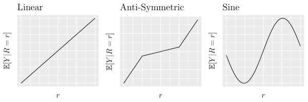
Figure 4: Data-generating models (DGMs) for the polynomial simulation.

When $Y$ may not be linear in $R$, flexibility in the $\mu_{\bm{\theta}}(R)$ function takes on added importance. We ran an additional simulation to explore the potential of robust polynomial regression to mitigate influence, as discussed in § 3.4 above, while adding flexibility to the specification of the $Y_{C}$ on $R$ regression. We compared limitless RD analysis, with $\mu_{\bm{\theta}}$ a polynomial in $R$ with degree 1, 2, 3, 4, or 5 to analogous estimates from OLS. In the OLS regressions, we followed the advice of Lee  Lemieux (e.g. 2010 , p. 318) and included interactions between the $R$-polynomial and $Z$. Finally, we compared these methods to local-linear regression with the triangular kernel and the bandwidth of Imbens  Kalyanaraman (2012). The OLS and limitless methods used the entire range of data. We simulated data sets of size $n=500$ by drawing $R$ and $\epsilon$ from Uniform $(-1,1)$ and $t_{3}$ distributions respectively, then adding $\epsilon$ to one of the three functions of $R$ shown in Figure 4 to form $Y_{C}$.

Table 4 displays the results. For the linear data-generating model, all estimates were unbiased, while root mean squared errors (RMSEs) were lowest for the limitless method. For the non-linear data-generating models, the limitless estimators using linear and quadratic specifications had substantial bias, and bias was much lower for higher-order polynomial specifications. In contrast, OLS estimators of all polynomial degrees were heavily biased. The local linear model does not employ higher-order polynomials. It fared better than OLS, having similar bias but higher RMSE than limitless with higher-order polynomials.

OLS and limitless estimation sharply diverge in the quality of their point estimates, with the OLS estimates’ RMSEs exceeding those of comparable robust M-estimates by factors exceeding 200. As Gelman  Imbens (2018) would predict, OLS estimates’ RMSEs increased sharply with each increment of polynomial degree, whatever the form of the data-generating model. In marked contrast, under non-linear data-generating models, higher-degree polynomial terms increased the accuracy of the robust, limitless method; under linear data-generating models, including higher-degree terms imposed little penalty.

6 Discussion

Beginning with Thistlethwaite  Campbell (1960), the dominant mode of RDD analysis has built upon ancova models. A modern variant instead targets parameters defined in terms of limits as $r\rightarrow c$, such as the LATE. However, in RDDs with discrete running variables such as LSO’s, neither $\lim_{r\downarrow 0}\mathbb{E}(Y|R=r)$ nor $\lim_{r\uparrow 0}\mathbb{E}(Y|R=r)$ exists, except perhaps as $\mathbb{E}(Y|R=-.01)$ or $\mathbb{E}(Y|R=0)$. A separate embarrassment for limit-based modeling of RDDs occurs if a donut-shaped $\mathcal{W}$ is necessary to address potential manipulation of the running variable, as we found to occur with the LSO data.

An alternative approach (e.g. Cattaneo ., 2015; Li ., 2015) takes the “local randomization” heuristic more literally, analyzing data in a small region around the cutoff as if it were from a randomized experiment. However, this approach assumes that potential outcomes are independent of $R$ in a window around the cutoff. That assumption is plausible of neither the Hurricane Maria example nor the LSO case study. In both settings, it is necessary to acknowledge and model the $R$–$Y$ relationship in order to set the stage for a credible claim of independence. The method of Cattaneo . (2015) performed poorly in our simulations (§ 5); its discrepant estimate of LSO’s AP effect (Table 2) embodies systematic error.

In contrast, this paper’s RDD analysis framework links ancova- and local randomization heuristics. Residual ignorability (5) assumes that the component of $Y_{c}$ that depends on $R$ may be modeled and removed, leaving residuals $e_{{\theta}_{0}}(\bm{Y}|{\bm{R}})$ that are independent of $Z$. Like the local randomization approach, it targets the TOTE or ATE within $\mathcal{W}$, as opposed to a difference of limits, and accommodates discreteness in $R$ and donut designs. In the special case of residual ignorability models with $e_{\theta}(\bm{Y}_{C}|{\bm{R}})\equiv\bm{Y}_{C}$ in (5), it reduces to the local randomization method. Like the limit-based approach, it models and accounts for the correlation between $R$ and $Y$. Under certain modeling and fitting choices, it returns the classical ancova estimate (§ 2.1).

The method of this paper improves upon each of these approaches by using robust M-estimation to adjust for $R$. For analysis of potentially imperfect RDDs, we see this as a necessity. For instance, covariate balance tests will necessarily be underpowered to detect imbalance in a small fraction of the sample, so the proper bandwidth $b$ will be uncertain. Likewise, if the initial sample includes subjects who manipulated their recorded $R$ values, then the use of donut-shaped $\mathcal{W}$ may remove some, but not all such subjects. Robust M-estimation retains consistency under scenarios such as these, with moderate amounts of contamination (He, 1991; Yohai  Zamar, 1997), whereas OLS does not.

If a large fraction of the dataset violates (5), even robust M-estimators can be misled. Thus, these methods should be used in addition to, rather than instead of, preliminary specification checks.

In simulated RDDs of moderate size, our estimates were unbiased and our confidence intervals were typically narrower than those from an OLS-based approach, while achieving nominal coverage. Further simulations found robust M-estimation to be compatible with the use of global cubic and quartic polynomials to accommodate nonlinear, imperfectly modeled relationships between $R$ and $Y_{C}$, in marked contrast to methods using OLS to adjust for trend.

Appendix A Large-sample randomization inference for RDDs

In Section 3 and following, the conditioning is with respect to

$$\mathcal{F}^{*}_{n}=\sigma\left[e_{{\theta}_{0}}(\mathbf{Y}_{C}|{\mathbf{R}}),\mathbf{D}_{T},\{(Y_{Ti},Y_{Ci},D_{Ti},R_{i})\mathcal{I}\left[{R}_{i}\not\in\mathcal{W}\right]\}_{i=1}^{n}\right],$$ (6)

a sigma field bearing information about $Y_{C}$s but not $Y_{T}$s. In contrast to sigma fields used in Fisherian randomization inference, it does not carry information about the sizes of the treatment and control groups (within $\{i:R_{i}\in\mathcal{W}\}$). In (6), conditioning on full information about subjects $i$ whose $R$ values fell outside $\mathcal{W}$ is a formal reflection of those subjects’ removal from the analytic sample.

As indicated in § 1.1, we assume non-interference, the model that a subject’s response may depend on his but not also on other subjects’ treatment assignments (Cox, 1958; Rubin, 1978); for fuzzy RDDs we also assume the exclusion restriction and monotonicity (of $(D_{C},D_{T})$). In varying degree, the sections that follow place additional assumptions bounding $Y_{T}$, $Y_{C}$ or transformations of them.

The Residual Ignorability condition of § 3.1 assumes $\hat{\theta}$ to be determined in a “sufficiently regular” fashion, noting that bounded influence MM-estimation meets this requirement. A weaker regularity condition than boundedness of the influence function is that the fitter’s influence function $\mathrm{IF}_{\hat{\theta}}(w,(\theta,\eta))$, where $(\theta,\eta)$ denotes the full parameter and $w=({y},d,r)$, must satisfy: $\mathbb{E}[\mathrm{IF}_{\hat{\theta}}(W,(\theta,\eta))]=0$ for a unique $\theta={\theta}_{0}$; each solution of $\mathbb{E}[\mathrm{IF}_{\hat{\theta}}(W,(\theta,\eta))]=0$ makes $\mathbb{E}[\mathrm{IF}_{\hat{\theta}}(W,(\theta,\eta))\mathrm{IF}_{\hat{\theta}}(W,(\theta,\eta))^{\prime}]$ finite.

A.1 Distributional approximation for $\hat{\theta}-{\theta}_{0}$

Recall Section 3.1 assumes that for the true parameter $({\theta}_{0},{\eta}_{0})$, $\mathbb{E}[\mathrm{IF}_{\hat{\theta}}(W,({\theta}_{0},{\eta}_{0}))]=0$ and $\Sigma=\mathbb{E}[\mathrm{IF}_{\hat{\theta}}(W,({\theta}_{0},{\eta}_{0}))\mathrm{IF}_{\hat{\theta}}(W,({\theta}_{0},{\eta}_{0}))^{\prime}]$ is finite. As noted by Stefanski  Boos (2002 § 3), these entail that $n^{-1/2}\sum_{i=1}^{n}\mathrm{IF}_{\hat{\theta}}(W_{i},({\theta}_{0},{\eta}_{0}))\stackrel{{\scriptstyle d}}{{\rightarrow}}N(0,\Sigma)$ and $n^{1/2}(\hat{\theta}-{\theta}_{0})\stackrel{{\scriptstyle d}}{{\rightarrow}}N(0,\Sigma)$, and if fitting is done by MM-estimation also that sandwich estimates are consistent, for $\Sigma$. This argument applies also if $\mathrm{IF}_{\hat{\theta}}(W_{i},({\theta}_{0},{\eta}_{0}))$ is the influence function of $(\hat{\theta},\hat{\gamma})$, as opposed only to $\hat{\theta}$, where $\hat{\gamma}$ is a $Z$-coefficient as discussed in Section 3.4.

For inference conditioned on $\mathcal{F}_{n}^{*}$ as in (6), we require an approximation to the distribution of $\sum_{i=1}^{n}\mathrm{IF}_{\hat{\theta}}(W_{i},({\theta}_{0},{\eta}_{0}))-\mathbb{E}[\mathrm{IF}_{\hat{\theta}}(W_{i},({\theta}_{0},{\eta}_{0}))|\mathcal{F}_{n}^{*}]$. For methods recommended in this paper, it suffices to consider the case that $\mathrm{IF}_{\hat{\theta}}(w,(\theta,\eta))$ is bounded. Write

$$\mathcal{G}_{n}=\sigma\left(\{W_{i}\}_{i=1}^{n};\{\left(e_{{\theta}_{0}}(\mathbf{Y}_{C}|{\mathbf{R}}),\mathbf{D}_{Ti},(Y_{Ti},Y_{Ci},D_{Ti},R_{i})\mathcal{I}\left[{R}_{i}\not\in\mathcal{W}\right]\right)\}_{i=n+1}^{\infty}\right)$$

so that $\mathcal{F}_{n}^{*}\subseteq\mathcal{G}_{m}$ for all $n$ and $m$, while $\sum_{i=1}^{n}\mathrm{IF}_{\hat{\theta}}(W_{i},({\theta}_{0},{\eta}_{0}))-\mathbb{E}[\mathrm{IF}_{\hat{\theta}}(W_{i},({\theta}_{0},{\eta}_{0}))|\mathcal{F}_{n}^{*}]$ is adapted to filtration $(\mathcal{G}_{n}:n)$. Fixing a vector $t$ of the same dimension as $\mathrm{IF}_{\hat{\theta}}(W_{i},({\theta}_{0},{\eta}_{0}))$, and writing $M_{n}=\sum_{i=1}^{n}t\mathrm{IF}_{\hat{\theta}}(W_{i},({\theta}_{0},{\eta}_{0}))-t\mathbb{E}[\mathrm{IF}_{\hat{\theta}}(W_{i},({\theta}_{0},{\eta}_{0}))|\mathcal{F}_{n}^{*}]$, we see that $(M_{n}:n)$ is a martingale. If $\mathrm{IF}_{\hat{\theta}}(W_{n},({\theta}_{0},{\eta}_{0}))t$ is $\mathcal{F}_{n}^{*}$-measurable then $M_{n}=0$ a.s. for all $n$, and is asymptotically $\mathrm{Normal}(0,0^{2})$. Otherwise $\mathbb{E}\{\mathrm{Var}[t\mathrm{IF}_{\hat{\theta}}(W_{i},({\theta}_{0},{\eta}_{0}))|\mathcal{F}_{n}^{*}]\}>0$ and $\sum\mathrm{Var}[t\mathrm{IF}_{\hat{\theta}}(W_{i},({\theta}_{0},{\eta}_{0}))|\mathcal{F}_{n}^{*}]=O_{P}(n)$. The Lindeberg condition follows by dominated convergence, since $\mathrm{IF}_{\hat{\theta}}(w,(\theta,\eta))$ is bounded. Thus $\{n^{1/2}M_{n}\}$ is asymptotically Normal by Lévy’s martingale central limit theorem. Because $t$ was arbitrary, it follows that $n^{-1/2}\sum_{i=1}^{n}t\mathrm{IF}_{\hat{\theta}}(W_{i},({\theta}_{0},{\eta}_{0}))-\mathbb{E}[t\mathrm{IF}_{\hat{\theta}}(W_{i},({\theta}_{0},{\eta}_{0}))|\mathcal{F}_{n}^{*}]$ converges in distribution to a Normal distribution with mean 0 and variance $\mathrm{Var}(t\mathrm{IF}_{\hat{\theta}}(W_{1},({\theta}_{0},{\eta}_{0}))\mid\mathcal{F}_{1}^{*})$. Accordingly $n^{1/2}(\hat{\theta},\hat{\gamma})-({\theta}_{0},{\gamma}_{0})$ is asymptotically MVN with covariance $\mathrm{Cov}[\mathrm{IF}_{\hat{\theta}}(W_{1},({\theta}_{0},{\eta}_{0}))\mid\mathcal{F}_{1}^{*}]$.

Sandwich covariance estimates converge to $\Sigma$, not $\mathrm{Cov}[\mathrm{IF}_{\hat{\theta}}(W_{1},({\theta}_{0},{\eta}_{0}))\mid\mathcal{F}_{1}^{*}]$; but since $t\mathrm{Cov}[\mathrm{IF}_{\hat{\theta}}(W_{1},({\theta}_{0},{\eta}_{0}))\mid\mathcal{F}_{1}^{*}]t^{\prime}\leq t\mathrm{Cov}[\mathrm{IF}_{\hat{\theta}}(W_{1},({\theta}_{0},{\eta}_{0}))]t^{\prime}$ for each $t$, under $H$ we have $\hat{\gamma}_{H}/\mathrm{SE}_{s}(\hat{\gamma}_{H})\stackrel{{\scriptstyle d}}{{\rightarrow}}\mathrm{Normal}(0,v)$ for some $v\leq 1$ (where “$\mathrm{SE}_{s}$” indicates a sandwich estimate).

A.2 Equivalence of tests from $z$-coefficent and from mean difference of partial residuals

Let $f_{0}(r)=1$, $f_{1}(r)=\mathcal{I}\left[r<0\right]-\mathbb{E}\mathcal{I}\left[R<0\right]=z-p_{z}$, and $f_{j}(\cdot)$, $j=2,\ldots,J$ be functions defining a design matrix for regression on $Z$ and $R$; denote coefficients of this regression $\alpha$, $\gamma$, $\beta$, where $\alpha$ and $\gamma$ are scalar coefficients for $f_{0}(r)$, $f_{1}(r)$ and $\beta$ is a scalar ($J=2$) or column vector ($J>2$) multiplier for row vectors $\vec{f}(r)=[f_{2}(r)\,\ldots\,f_{J}(r)]$. We demonstrate that when $\alpha$, $\gamma$, $\beta$ and perhaps other components of $\theta$ are fitted simultaneously, in an MM-estimation type regression procedure making their sampling variability $O_{P}(n^{-1/2})$, then $\hat{\gamma}$ differs only by $o_{P}(n^{-1/2})$ from a constant multiple of $\overline{e_{\hat{\theta}}(y_{H}|{r})}_{z=1}-\overline{e_{\hat{\theta}}(y_{H}|{r})}_{z=0}$, the difference in means of partial residuals.

Denote parameters other than $\gamma$, i.e. $\alpha$, $\beta$, a scale parameter $s$ and perhaps others, collectively by $\eta$, so that $\theta=(\gamma,\eta)$. Fixing a (strong) hypothesis $H$, write ${w}$ for $({y}_{H},{r},z)$ and $e_{(\gamma,\eta)}(w)$ for $\psi\{(y_{H}-\alpha-\gamma f_{1}(r)-\vec{f}(r)\beta)/s\}$ such that the estimating functions are $\Psi_{j}(w,\gamma,\eta)=e_{(\gamma,\eta)}(w)f_{j}(r)$, $j\leq J$. The column equation $\mathbb{E}\Psi(W,\gamma_{H},\eta_{H})=0$, $\Psi(w,\gamma,\eta)=[\Psi_{1}(w,\gamma,\eta),\ldots,\Psi_{J}(w,\gamma,\eta)]^{t}$, implicitly defines $\gamma_{H}$, and defines or contributes to an implicit definition of $\theta_{H}$. It’s permitted that there be additional estimating equations, not involving $\gamma$, that contribute to the implicit definition of $\theta$: in robust regression, equations defining the preliminary scale estimate; an equation $\mathbb{E}Z=p_{z}$ defining $p_{z}$. Note that $\Psi_{1}$’s $z$-factor has been centered around $p_{z}$. This facilitates the argument by ensuring that $\sum_{i}\Psi_{1}(W_{i},\gamma,\eta)=np_{z}(1-p_{z})\{\overline{e_{(\gamma,\eta)}(W)}_{Z=1}-\overline{e_{(\gamma,\eta)}(W)}_{Z=0}\}$, but does not affect the value of $\gamma$ or its estimates $\hat{\gamma}$, due to the inclusion via $\Psi_{0}$ of an intercept term. Note that $e_{\theta}({y_{H}}|{r})=e_{(\gamma,\eta)}({y_{H}}|{r})=e_{(0,\eta)}(w)$.

Finally, assume that with these estimating equations and $\mathcal{L}(W)$ jointly the estimating function is asymptotically linear,

$$n^{-1}\sum_{i=1}^{n}\Psi(W_{i},\hat{\gamma}_{n},\hat{\eta}_{n})\\ =n^{-1}\sum_{i=1}^{n}\Psi(W_{i},\gamma_{H},\eta_{H})+\dot{\Psi}_{H}\,[\hat{\gamma}_{n}-\gamma_{H},\hat{\eta}_{n}-\eta_{H}]^{t}+o_{P}(n^{-1/2})$$ (7)

for consistent estimators $(\hat{\gamma}_{n},\hat{\eta}_{n})$ of $(\gamma_{H},\eta_{H})$, where $\dot{\Psi}_{H}$ is a matrix with rows $\nabla_{\gamma,\eta}\{\mathbb{E}\Psi_{j}(W,\gamma,\eta)\}$, as evaluated at ${(\gamma,\eta)=(\gamma_{H},\eta_{H})}$. Assume the fitting procedure generates consistent estimators of $(\gamma_{H},\eta_{H})$ and $\dot{\Psi}_{H}$, denoted $(\hat{\gamma},\hat{\eta})$ and $\hat{\dot{\Psi}}$, with either $\sum_{i=1}^{n}\Psi(W_{i},\hat{\gamma},\hat{\eta})=0$ or at least $|\sum_{i=1}^{n}\Psi(W_{i},\hat{\gamma},\hat{\eta})|_{2}=o_{P}(n^{-1/2})$.

For robust regression embodying a residual transformation $\psi(\cdot)$ that redescends, consistency and (7) follow if $\Psi$ is twice differentiable in the parameters, with derivatives of $\Psi(W,\gamma,\beta,\sigma)$ bounded by a function $K(W)$ with finite expectation. This can be assumed of robust regression using the bisquare or lqq $\psi$ functions, as in R’s robustbase package or Stata’s mmregress, if ${Y_{H}}$ and $(f_{j}(R):j)$ have finite second moments. If $\Psi$ is the estimating function of an ordinary or generalized linear model, or robust regression with Huber loss, suitable conditions for consistency and (7) are given in e.g. He  Shao (2000).

If $H$ is true then $\gamma_{H}=0$, and either of $(\hat{\gamma},\hat{\eta})$ and $(0,\hat{\eta})$ is consistent for $(\gamma_{H},\eta_{H})=(0,\eta_{H})$. Under $H$, then, we can apply (7) to either of these estimator sequences, with the consequence that

$$n^{-1}\sum_{i=1}^{n}\Psi_{1}(W_{i},\hat{\gamma},\hat{\eta})- n^{-1}\sum_{i=1}^{n}\Psi_{1}(W_{i},0,\hat{\eta})$$

$$=\left[\frac{\partial}{\partial\gamma}\mathbb{E}\Psi_{1}(W,\gamma,\eta)|_{(0,\eta_{H})}\right]\hat{\gamma}+o_{P}(n^{-1/2})$$

$$={\dot{\Psi}}_{1\gamma}\hat{\gamma}+o_{P}(n^{-1/2}).$$

Since $n^{-1}|\sum_{i=1}^{n}\Psi(W_{i},\hat{\gamma},\hat{\eta})|_{2}=o_{P}(n^{-1/2})$, this means that up to differences of order $o_{P}(n^{-1/2})$, $n^{-1}\sum_{i=1}^{n}\Psi_{1}(W_{i},0,\hat{\eta})\approx\dot{\Psi}_{1\gamma}\hat{\gamma}$. But $n^{-1}\sum_{i=1}^{n}\Psi_{1}(W_{i},0,\hat{\eta})=\bar{z}(1-\bar{z})\{\overline{e_{(0,\hat{\eta})}(W)}_{Z=1}-\overline{e_{(0,\hat{\eta})}(W)}_{Z=0}\}$, so

$$n^{1/2}\left|\frac{\bar{z}(1-\bar{z})}{\hat{\dot{\Psi}}_{1\gamma}}\cdot\left[\overline{e_{(0,\hat{\eta})}(W)}_{Z=1}-\overline{e_{(0,\hat{\eta})}(W)}_{Z=0}\right]-\hat{\gamma}\right|\stackrel{{\scriptstyle P}}{{\rightarrow}}0.$$

A.3 Differences of residual means involving parameters estimated during detrending

Fix $H:Y_{T}=Y_{C}+\tau_{0}D_{T}$ and write

$${Y}_{HC}={Y}_{T}-{D}_{T}\tau_{0}\quad\text{and}\quad Y_{H}=ZY_{HC}+(1-Z)Y_{C},$$ (8)

so that for each $i$ ${Y}_{HCi}$ is the $y_{C}$-value that would be reconstructed from data $(y_{Ti},d_{Ti})$ under $H$, if $(y_{Ti},d_{Ti})$ rather than $y_{Ci}$ were observed, whereas $\mathbf{y}_{H}$ is the reconstruction of $\mathbf{y}_{C}$ according to $H$ based on those data that were actually observed. Thus $\mathbf{Y}_{HC}\equiv\mathbf{Y}_{C}$ if $H$ is true, but not otherwise. Let $\bar{\theta}=(\bar{\alpha},\bar{\beta},\bar{s},\ldots)$ describe a solution of a system of estimating equations, including a subsystem $\mathbb{E}\psi\{(Y_{H}-\vec{f}(R)(\alpha,\beta))/s\}\vec{f}(R)=\mathbf{0}$, some $\vec{f}(\cdot)=[f_{0}(\cdot)\,f_{1}(\cdot)\,\ldots\,f_{k}(\cdot)]$ and some $\psi(\cdot)$. (For $n$-vectors $\mathbf{u}$, $\mathbf{v}$, and $\mathbf{x}$, “$[\mathbf{u}\,\mathbf{v}\,\mathbf{x}]$” denotes the $n\times 3$ matrix with columns $\mathbf{u}$, $\mathbf{v}$, and $\mathbf{x}$.) In the method described and exemplified in Section 3 and subsequent parts of the paper, $e_{\theta}(y_{H}|{r})=\psi\{(y_{H}-\vec{f}(r)(\alpha,\beta))/s\}$; however, for the arguments presented in this appendix it is permitted that $\theta$ be estimated using an unrelated $\psi(\cdot)$ function, prior to and separately from the residualization $(y,r)\mapsto e_{\theta}(y|{r})$ figuring in tests of $H$.

Given modest regularity conditions on the distribution of $(Y_{H},R)=(Zy_{HC}+(1-Z)y_{C},R)$ (cf. (8)) and the transformation $e_{\theta}(\cdot|{\cdot})$, one has

$$\{\overline{e_{\hat{\theta}}(Y_{H}|{{R}})}_{Z=1}-\overline{e_{\hat{\theta}}(Y_{H}|{{R}})}_{Z=0}\}-\{\overline{e_{\bar{\theta}}(Y_{H}|{{R}})}_{Z=1}-\overline{e_{\bar{\theta}}(Y_{H}|{{R}})}_{Z=0}\}=\\ \nabla_{\theta}\bigg{[}\mathbb{E}\Big{\{}e_{\theta}({{Y}_{H}}|{{R}})\Big{|}Z=1\Big{\}}-\mathbb{E}\Big{\{}e_{\theta}({{Y}_{H}}|{{R}})\Big{|}Z=0\Big{\}}\bigg{]}_{\theta=\bar{\theta}}(\hat{\theta}-\bar{\theta})^{t}+o_{P}(n^{-1/2}),$$ (9)

where $\bar{\theta}=\mathbb{E}(\hat{\theta}({\mathbf{Y}_{H}},\mathbf{R}))$; see Proposition 1 below. When $\hat{\theta}$ is $n^{1/2}$-consistent and asymptotically Normal, this relationship warrants the use of Huber-White estimates of $\mathrm{Var}\left\{\overline{e_{\hat{\theta}}(Y_{H}|{{R}})}_{Z=1}-\overline{e_{\hat{\theta}}(Y_{H}|{{R}})}_{Z=0}\right\}$, in turn providing a basis for large-sample t-tests.

Approximation (9) holds for randomized and quasiexperimental designs alike, but in RCTs the bracketed difference of expectations vanishes under $H$ (Hansen  Bowers, 2009; Lin, 20131, 20132), and the product at right of (9) vanishes as well. Up to $o_{P}(n^{-1})$, the variances $\mathrm{Var}\left\{\overline{e_{\hat{\theta}}({Y_{H}}|{R})}_{Z=1}-\overline{e_{\hat{\theta}}({Y_{H}}|{R})}_{Z=0}\right\}$ and $\mathrm{Var}\left\{\overline{e_{\bar{\theta}}({Y_{H}}|{R})}_{Z=1}-\overline{e_{\bar{\theta}}({Y_{H}}|{R})}_{Z=0}\right\}$ are the same, the latter being no greater than the expected value of the squared standard error of two-sample inference with unequal variances, as applied to $e_{\bar{\theta}}({y_{H}}|{r})$. In practice that specific standard error is unavailable, $\bar{\theta}$ being unknown; but its ratio with $\mathrm{SE}_{u}\big{\{}\overline{e_{\theta}({Y_{H}}|{R})}_{Z=1}-\overline{e_{\theta}({Y_{H}}|{R})}_{Z=0}\big{\}}\big{|}_{\theta=\hat{\theta}}$, the unequal-variances two-sample standard error as figured with substitution of $\hat{\theta}$ for $\theta$, tends in probability to 1, by Slutsky’s Lemma; this suffices for the limiting null distribution of the Studentized $t$-statistic to be standard Normal. So in an RCT there is no need for any explicit acknowledgment of sampling variability in $\hat{\theta}$.

But this argument does not extend to RDDs. Rather, in an RDD the expected values compared in (9) coincide only for a single value, ordinarily 0, of $\theta$’s slope component. The differential at right of (9) is generally nonzero; it must be permitted to make a contribution. Fortunately any ordinary standard error attaching to the $z$-coefficient of the regression of ${\mathbf{Y}_{H}}$ on $\mathbf{1}$, $\mathbf{R}$ and $\mathbf{Z}$ will do so; this includes Huber-White standard errors.

Let $\theta\mapsto e_{\theta}(y|{y})=e_{\theta}(w)$ be continuously differentiable (for each $w=(y,{r})$). By the mean value theorem,

$$\big{\{}[\overline{e_{\hat{\theta}}({w})}_{z=1}-\overline{e_{\bar{\theta}}({w})}_{z=1}]-[\overline{e_{\hat{\theta}}({w})}_{z=0}-\overline{e_{\bar{\theta}}({w})}_{z=0}]\big{\}}\\ =\nabla_{\theta}\big{[}\overline{e_{\theta}({w})}_{z=1}-\overline{e_{\theta}({w})}_{z=0}\big{]}_{\begin{subarray}{c}\theta=\theta^{*}\end{subarray}}\cdot(\hat{\theta}-\bar{\theta}),$$ (10)

some $\theta^{*}$ on the line segment connecting $\hat{\theta}$ and $\bar{\theta}$. Of course $\theta^{*}\stackrel{{\scriptstyle P}}{{\rightarrow}}\bar{\theta}$ if $\hat{\theta}\stackrel{{\scriptstyle P}}{{\rightarrow}}\bar{\theta}$.

Let there be a compact neighborhood $\Theta$ of $\bar{\theta}$ and an accompanying envelope function $k_{\Theta}(\cdot)$, i.e., $|\nabla_{\theta}e_{\theta}(w)|\leq k_{\Theta}(w)$, all $\theta\in\Theta$ and all $w$, that is integrable, $\mathbb{E}k_{\Theta}(W)<\infty$. With this assumption, the uniform strong law (e.g., Ferguson, 1996 Ch.16) entails that if $\theta^{*}\stackrel{{\scriptstyle P}}{{\rightarrow}}\bar{\theta}$ then

$$\overline{\big{(}\nabla_{\theta}e_{\theta}({w})|_{\theta=\theta^{*}}\big{)}}_{Z=z}\stackrel{{\scriptstyle P}}{{\rightarrow}}\mathbb{E}\big{[}\nabla_{\theta}e_{\theta}(W)|_{\theta=\bar{\theta}}\big{|}Z=z\big{]},\,z=0\,\mathrm{or}\,1.$$ (11)

Moreover, since there is an integrable envelope function, dominated convergence and the mean value theorem combine to warrant interchanging the expected value and differentiation operations at right of (11).

Strengthening the consistency assumption on $\hat{\theta}$ to root-n consistency, $|\hat{\theta}-\bar{\theta}|_{2}=O_{P}(n^{-1/2})$, it now follows that the difference of the right-hand side of (10) and

$$\nabla_{\theta}\bigg{\{}\mathbb{E}\big{[}e_{\theta}(W)\big{|}Z=1\big{]}-\mathbb{E}\big{[}e_{\theta}(W)\big{|}Z=0\big{]}\bigg{\}}_{\theta=\bar{\theta}}\cdot(\hat{\theta}-\bar{\theta})$$ (12)

is $o_{P}(n^{-1/2})$. This suffices for (9). To summarize:

Proposition 1.

Under (1)–(3) below, $n^{1/2}\{$ (12) $-$ RHS of (10)}$\stackrel{{\scriptstyle P}}{{\rightarrow}}0$ as $n\uparrow\infty$, and in consequence (9) holds.

1. for each $(y,r)$, $\nabla_{\theta}e_{\theta}(y|{r})$ exists and is continuous in $\theta$;

2. for some compact $\Theta$, open $S\subseteq\Theta$ with $\bar{\theta}\in S$, and $k_{\Theta}(\cdot,\cdot)$ with $\mathbb{E}k_{\Theta}({Y_{H}},R)<\infty$, $|\nabla_{\theta}e_{\theta}(y|{r})|\leq k_{\Theta}(y,r)$ for all $(y,r)$; and

3. $|\hat{\theta}-\bar{\theta}|_{2}=O_{P}(n^{-1/2})$.

The argument can be generalized to cover residual transformations that are Lipschitz but not continuously differentiable in $\theta$, but the generalization is not needed for ordinary generalized linear model fitters, nor for common bounded-influence alternatives (e.g., robust regression with bisquare psi function).

References

- Agresti (\APACyear2011) \APACinsertmetastaragresti2011scoreintervals{APACrefauthors}Agresti, A. \APACrefYearMonthDay2011. \BBOQ\APACrefatitleScore and pseudo-score confidence intervals for categorical data analysis Score and pseudo-score confidence intervals for categorical data analysis.\BBCQ \APACjournalVolNumPagesStatistics in Biopharmaceutical Research32163–172. \PrintBackRefs\CurrentBib
- Agresti \BBA Gottard (\APACyear2005) \APACinsertmetastaragresti2005comment{APACrefauthors}Agresti, A.\BCBT \BBA Gottard, A. \APACrefYearMonthDay2005. \BBOQ\APACrefatitleComment: Randomized confidence intervals and the mid-p approach Comment: Randomized confidence intervals and the mid-p approach.\BBCQ \APACjournalVolNumPagesStatistical Science204367–371. \PrintBackRefs\CurrentBib
- Angrist \BOthers. (\APACyear1996) \APACinsertmetastarAngrist:etal:1996{APACrefauthors}Angrist, J\BPBID., Imbens, G\BPBIW.\BCBL \BBA Rubin, D\BPBIB. \APACrefYearMonthDay1996June. \BBOQ\APACrefatitleIdentification of causal effects using instrumental variables Identification of causal effects using instrumental variables.\BBCQ \APACjournalVolNumPagesJournal of the American Statistical Association91434444–455. \PrintBackRefs\CurrentBib
- Angrist \BBA Lavy (\APACyear1999) \APACinsertmetastarangrist1999using{APACrefauthors}Angrist, J\BPBID.\BCBT \BBA Lavy, V. \APACrefYearMonthDay1999. \BBOQ\APACrefatitleUsing Maimonides’ rule to estimate the effect of class size on scholastic achievement Using Maimonides’ rule to estimate the effect of class size on scholastic achievement.\BBCQ \APACjournalVolNumPagesThe Quarterly Journal of Economics1142533–575. \PrintBackRefs\CurrentBib
- Aronow \BOthers. (\APACyear2016) \APACinsertmetastararonowRDDinterference{APACrefauthors}Aronow, P\BPBIM., Basta, N\BPBIE.\BCBL \BBA Halloran, M\BPBIE. \APACrefYearMonthDay2016. \BBOQ\APACrefatitleThe Regression Discontinuity Design Under Interference: A Local Randomization-based Approach The regression discontinuity design under interference: A local randomization-based approach.\BBCQ \APACjournalVolNumPagesObservational Studies2129-133. \PrintBackRefs\CurrentBib
- Baiocchi \BOthers. (\APACyear2014) \APACinsertmetastarbaiocchiChengSmall2014IVtutorial{APACrefauthors}Baiocchi, M., Cheng, J.\BCBL \BBA Small, D\BPBIS. \APACrefYearMonthDay2014. \BBOQ\APACrefatitleInstrumental variable methods for causal inference Instrumental variable methods for causal inference.\BBCQ \APACjournalVolNumPagesStatistics in Medicine33132297–2340. \PrintBackRefs\CurrentBib
- Barreca \BOthers. (\APACyear2011) \APACinsertmetastarbarrecaetal2011birthweightRDD{APACrefauthors}Barreca, A\BPBII., Guldi, M., Lindo, J\BPBIM.\BCBL \BBA Waddell, G\BPBIR. \APACrefYearMonthDay2011. \BBOQ\APACrefatitleSaving babies? Revisiting the effect of very low birth weight classification Saving babies? Revisiting the effect of very low birth weight classification.\BBCQ \APACjournalVolNumPagesThe Quarterly Journal of Economics12642117–2123. \PrintBackRefs\CurrentBib
- Bell \BBA McCaffrey (\APACyear2002) \APACinsertmetastarbellmccaffrey2002sandwichSEs{APACrefauthors}Bell, R\BPBIM.\BCBT \BBA McCaffrey, D\BPBIF. \APACrefYearMonthDay2002. \BBOQ\APACrefatitleBias reduction in standard errors for linear regression with multi-stage samples Bias reduction in standard errors for linear regression with multi-stage samples.\BBCQ \APACjournalVolNumPagesSurvey Methodology282169–182. \PrintBackRefs\CurrentBib
- Berk \BBA Rauma (\APACyear1983) \APACinsertmetastarberk1983capitalizing{APACrefauthors}Berk, R\BPBIA.\BCBT \BBA Rauma, D. \APACrefYearMonthDay1983. \BBOQ\APACrefatitleCapitalizing on nonrandom assignment to treatments: A regression-discontinuity evaluation of a crime-control program Capitalizing on nonrandom assignment to treatments: A regression-discontinuity evaluation of a crime-control program.\BBCQ \APACjournalVolNumPagesJournal of the American Statistical Association21–27. \PrintBackRefs\CurrentBib
- Bloom (\APACyear1984) \APACinsertmetastarbloom1984ans{APACrefauthors}Bloom, H\BPBIS. \APACrefYearMonthDay1984. \BBOQ\APACrefatitleAccounting for no-shows in experimental evaluation designs Accounting for no-shows in experimental evaluation designs.\BBCQ \APACjournalVolNumPagesEvaluation Review82225. \PrintBackRefs\CurrentBib
- Boos (\APACyear1992) \APACinsertmetastarboos1992genscoretest{APACrefauthors}Boos, D\BPBID. \APACrefYearMonthDay1992. \BBOQ\APACrefatitleOn generalized score tests On generalized score tests.\BBCQ \APACjournalVolNumPagesThe American Statistician464327–333. \PrintBackRefs\CurrentBib
- Calonico \BOthers. (\APACyear2014) \APACinsertmetastarcalonico2014robust{APACrefauthors}Calonico, S., Cattaneo, M\BPBID.\BCBL \BBA Titiunik, R. \APACrefYearMonthDay2014. \BBOQ\APACrefatitleRobust nonparametric confidence intervals for regression-discontinuity designs Robust nonparametric confidence intervals for regression-discontinuity designs.\BBCQ \APACjournalVolNumPagesEconometrica8262295–2326. \PrintBackRefs\CurrentBib
- Canay \BBA Kamat (\APACyear2017) \APACinsertmetastarcanayKamat17RDDpermutations{APACrefauthors}Canay, I\BPBIA.\BCBT \BBA Kamat, V. \APACrefYearMonthDay2017. \BBOQ\APACrefatitleApproximate permutation tests and induced order statistics in the regression discontinuity design Approximate permutation tests and induced order statistics in the regression discontinuity design.\BBCQ \APACjournalVolNumPagesThe Review of Economic Studies8531577–1608. \PrintBackRefs\CurrentBib
- Cattaneo \BOthers. (\APACyear2015) \APACinsertmetastarcattaneo2014randomization{APACrefauthors}Cattaneo, M\BPBID., Frandsen, B\BPBIR.\BCBL \BBA Titiunik, R. \APACrefYearMonthDay2015. \BBOQ\APACrefatitleRandomization inference in the regression discontinuity design: An application to party advantages in the US Senate Randomization inference in the regression discontinuity design: An application to party advantages in the US senate.\BBCQ \APACjournalVolNumPagesJournal of Causal Inference311–24. \PrintBackRefs\CurrentBib
- Cook \BBA Weisberg (\APACyear1982) \APACinsertmetastarcook1982residuals{APACrefauthors}Cook, R\BPBID.\BCBT \BBA Weisberg, S. \APACrefYear1982. \APACrefbtitleResiduals and influence in regression Residuals and influence in regression. \APACaddressPublisherChapman and Hall New York. \PrintBackRefs\CurrentBib
- Cox (\APACyear1958) \APACinsertmetastarcox:1958{APACrefauthors}Cox, D\BPBIR. \APACrefYear1958. \APACrefbtitleThe Planning of Experiments The planning of experiments. \APACaddressPublisherJohn Wiley. \PrintBackRefs\CurrentBib
- Cox (\APACyear2006) \APACinsertmetastarcox2006pos{APACrefauthors}Cox, D\BPBIR. \APACrefYear2006. \APACrefbtitlePrinciples of Statistical Inference Principles of statistical inference. \APACaddressPublisherCambridge University Press. \PrintBackRefs\CurrentBib
- Dimmery (\APACyear2013) \APACinsertmetastarrdd{APACrefauthors}Dimmery, D. \APACrefYearMonthDay2013. \BBOQ\APACrefatitlerdd: Regression Discontinuity Estimation rdd: Regression discontinuity estimation\BBCQ [\bibcomputersoftwaremanual]. {APACrefURL} http://CRAN.R-project.org/package=rdd \APACrefnoteR package version 0.54 \PrintBackRefs\CurrentBib
- Dong (\APACyear2015) \APACinsertmetastardong2015regression{APACrefauthors}Dong, Y. \APACrefYearMonthDay2015. \BBOQ\APACrefatitleRegression discontinuity applications with rounding errors in the running variable Regression discontinuity applications with rounding errors in the running variable.\BBCQ \APACjournalVolNumPagesJournal of Applied Econometrics303422–446. \PrintBackRefs\CurrentBib
- Eggers \BOthers. (\APACyear2015) \APACinsertmetastareggers2014validity{APACrefauthors}Eggers, A., Fowler, A., Hainmueller, J., Hall, A\BPBIB.\BCBL \BBA Snyder, J\BPBIM. \APACrefYearMonthDay2015. \BBOQ\APACrefatitleOn the validity of the regression discontinuity design for estimating electoral effects: New evidence from over 40,000 close races On the validity of the regression discontinuity design for estimating electoral effects: New evidence from over 40,000 close races.\BBCQ \APACjournalVolNumPagesAmerican Journal of Political Science591259–74. \PrintBackRefs\CurrentBib
- Ferguson (\APACyear1996) \APACinsertmetastarferguson1996largesampletheory{APACrefauthors}Ferguson, T\BPBIS. \APACrefYear1996. \APACrefbtitleA course in large sample theory A course in large sample theory. \APACaddressPublisherChapman & Hall London. \PrintBackRefs\CurrentBib
- Fisher (\APACyear1935) \APACinsertmetastarfisher:1935{APACrefauthors}Fisher, R\BPBIA. \APACrefYear1935. \APACrefbtitleDesign of Experiments Design of experiments. \APACaddressPublisherEdinburghOliver and Boyd. \PrintBackRefs\CurrentBib
- Frandsen (\APACyear2017) \APACinsertmetastarfrandsenTest{APACrefauthors}Frandsen, B\BPBIR. \APACrefYearMonthDay2017. \BBOQ\APACrefatitleParty bias in union representation elections: Testing for manipulation in the regression discontinuity design when the running variable is discrete Party bias in union representation elections: Testing for manipulation in the regression discontinuity design when the running variable is discrete.\BBCQ \BIn M\BPBID. Cattaneo \BBA J\BPBIC. Escanciano (\BEDS), \APACrefbtitleRegression Discontinuity Designs: Theory and Applications Regression discontinuity designs: Theory and applications (\BPGS 281–315). \APACaddressPublisherEmerald Publishing Limited. \PrintBackRefs\CurrentBib
- Freedman (\APACyear2006) \APACinsertmetastarfreedman2006sch{APACrefauthors}Freedman, D\BPBIA. \APACrefYearMonthDay2006. \BBOQ\APACrefatitleOn The So-Called “Huber Sandwich Estimator” and “Robust Standard Errors” On the so-called “Huber sandwich estimator” and “robust standard errors”.\BBCQ \APACjournalVolNumPagesThe American Statistician604299–302. \PrintBackRefs\CurrentBib
- Gelman \BBA Imbens (\APACyear2018) \APACinsertmetastargelman2016high{APACrefauthors}Gelman, A.\BCBT \BBA Imbens, G\BPBIW. \APACrefYearMonthDay2018. \BBOQ\APACrefatitleWhy High-order Polynomials Should not be Used in Regression Discontinuity Designs Why high-order polynomials should not be used in regression discontinuity designs.\BBCQ \APACjournalVolNumPagesJournal of Business and Economic Statistics. \PrintBackRefs\CurrentBib
- Hansen \BBA Bowers (\APACyear2009) \APACinsertmetastarbowers:hans:2008{APACrefauthors}Hansen, B\BPBIB.\BCBT \BBA Bowers, J. \APACrefYearMonthDay2009. \BBOQ\APACrefatitleAttributing Effects to A Cluster Randomized Get-Out-The-Vote Campaign Attributing effects to a cluster randomized get-out-the-vote campaign.\BBCQ \APACjournalVolNumPagesJournal of the American Statistical Association104487873–85. \PrintBackRefs\CurrentBib
- Hansen \BBA Sales (\APACyear2015) \APACinsertmetastarhansenSales2015cochran{APACrefauthors}Hansen, B\BPBIB.\BCBT \BBA Sales, A\BPBIC. \APACrefYearMonthDay2015. \BBOQ\APACrefatitleComments on “Observational Studies,” by William G. Cochran Comments on “Observational Studies,” by William G. Cochran.\BBCQ \APACjournalVolNumPagesObservational Studies11184-193. \PrintBackRefs\CurrentBib
- He (\APACyear1991) \APACinsertmetastarhe1991localbreakdown{APACrefauthors}He, X. \APACrefYearMonthDay1991. \BBOQ\APACrefatitleA local breakdown property of robust tests in linear regression A local breakdown property of robust tests in linear regression.\BBCQ \APACjournalVolNumPagesJournal of Multivariate Analysis382294–305. \PrintBackRefs\CurrentBib
- He \BBA Shao (\APACyear2000) \APACinsertmetastarhe2000parameters{APACrefauthors}He, X.\BCBT \BBA Shao, Q\BHBIM. \APACrefYearMonthDay2000. \BBOQ\APACrefatitleOn parameters of increasing dimensions On parameters of increasing dimensions.\BBCQ \APACjournalVolNumPagesJournal of Multivariate Analysis731120–135. \PrintBackRefs\CurrentBib
- Huber (\APACyear1964) \APACinsertmetastarhuber1964robust{APACrefauthors}Huber, P\BPBIJ. \APACrefYearMonthDay1964. \BBOQ\APACrefatitleRobust estimation of a location parameter Robust estimation of a location parameter.\BBCQ \APACjournalVolNumPagesThe Annals of Mathematical Statistics35173–101. \PrintBackRefs\CurrentBib
- Huber (\APACyear1967) \APACinsertmetastarhuber1967behavior{APACrefauthors}Huber, P\BPBIJ. \APACrefYearMonthDay1967. \BBOQ\APACrefatitleThe behavior of maximum likelihood estimates under nonstandard conditions The behavior of maximum likelihood estimates under nonstandard conditions.\BBCQ \BIn \APACrefbtitleProceedings of the fifth Berkeley symposium on mathematical statistics and probability Proceedings of the fifth berkeley symposium on mathematical statistics and probability (\BVOL 1, \BPGS 221–233). \PrintBackRefs\CurrentBib
- Imbens \BBA Kalyanaraman (\APACyear2012) \APACinsertmetastarimbens2012optimal{APACrefauthors}Imbens, G\BPBIW.\BCBT \BBA Kalyanaraman, K. \APACrefYearMonthDay2012. \BBOQ\APACrefatitleOptimal bandwidth choice for the regression discontinuity estimator Optimal bandwidth choice for the regression discontinuity estimator.\BBCQ \APACjournalVolNumPagesThe Review of Economic Studies793933–959. \PrintBackRefs\CurrentBib
- Imbens \BBA Lemieux (\APACyear2008) \APACinsertmetastarimbens2008regression{APACrefauthors}Imbens, G\BPBIW.\BCBT \BBA Lemieux, T. \APACrefYearMonthDay2008. \BBOQ\APACrefatitleRegression discontinuity designs: A guide to practice Regression discontinuity designs: A guide to practice.\BBCQ \APACjournalVolNumPagesJournal of Econometrics1422615–635. \PrintBackRefs\CurrentBib
- Imbens \BBA Rosenbaum (\APACyear2005) \APACinsertmetastarimbens:rose:2005{APACrefauthors}Imbens, G\BPBIW.\BCBT \BBA Rosenbaum, P\BPBIR. \APACrefYearMonthDay2005. \BBOQ\APACrefatitleRobust, Accurate Confidence Intervals with a Weak Instrument: Quarter of Birth and Education Robust, accurate confidence intervals with a weak instrument: Quarter of birth and education.\BBCQ \APACjournalVolNumPagesJournal of the Royal Statistical Society, Series A: Statistics in Society1681109–126. \PrintBackRefs\CurrentBib
- Imbens \BBA Wager (\APACyear2017) \APACinsertmetastarimbens2017optimized{APACrefauthors}Imbens, G\BPBIW.\BCBT \BBA Wager, S. \APACrefYearMonthDay2017. \BBOQ\APACrefatitleOptimized Regression Discontinuity Designs Optimized regression discontinuity designs.\BBCQ \APACjournalVolNumPagesarXiv preprint arXiv:1705.01677. \PrintBackRefs\CurrentBib
- Kolesár \BBA Rothe (\APACyear2018) \APACinsertmetastarkolesarRothe17{APACrefauthors}Kolesár, M.\BCBT \BBA Rothe, C. \APACrefYearMonthDay2018. \BBOQ\APACrefatitleInference in regression discontinuity designs with a discrete running variable Inference in regression discontinuity designs with a discrete running variable.\BBCQ \APACjournalVolNumPagesAmerican Economic Review10882277–2304. \PrintBackRefs\CurrentBib
- Lee (\APACyear2008) \APACinsertmetastarlee2008randomized{APACrefauthors}Lee, D\BPBIS. \APACrefYearMonthDay2008. \BBOQ\APACrefatitleRandomized experiments from non-random selection in US House elections Randomized experiments from non-random selection in us house elections.\BBCQ \APACjournalVolNumPagesJournal of Econometrics1422675–697. \PrintBackRefs\CurrentBib
- Lee \BBA Lemieux (\APACyear2010) \APACinsertmetastarlee2010regression{APACrefauthors}Lee, D\BPBIS.\BCBT \BBA Lemieux, T. \APACrefYearMonthDay2010. \BBOQ\APACrefatitleRegression Discontinuity Designs in Economics Regression discontinuity designs in economics.\BBCQ \APACjournalVolNumPagesJournal of Economic Literature48281–355. \PrintBackRefs\CurrentBib
- Li \BOthers. (\APACyear2015) \APACinsertmetastarliMatteiMealli2015BayesianRD{APACrefauthors}Li, F., Mattei, A.\BCBL \BBA Mealli, F. \APACrefYearMonthDay2015. \BBOQ\APACrefatitleEvaluating the causal effect of university grants on student dropout: Evidence from a regression discontinuity design using principal stratification Evaluating the causal effect of university grants on student dropout: Evidence from a regression discontinuity design using principal stratification.\BBCQ \APACjournalVolNumPagesThe Annals of Applied Statistics941906–1931. \PrintBackRefs\CurrentBib
- Lin (\APACyear2013\APACexlab\BCnt1) \APACinsertmetastarlin2013agnostic{APACrefauthors}Lin, W. \APACrefYearMonthDay2013\BCnt1. \BBOQ\APACrefatitleAgnostic notes on regression adjustments to experimental data: reexamining Freedman’s critique Agnostic notes on regression adjustments to experimental data: reexamining Freedman’s critique.\BBCQ \APACjournalVolNumPagesThe Annals of Applied Statistics71295–318. \PrintBackRefs\CurrentBib
- Lin (\APACyear2013\APACexlab\BCnt2) \APACinsertmetastarlin2013agnosticSupp{APACrefauthors}Lin, W. \APACrefYearMonthDay2013\BCnt2. \BBOQ\APACrefatitleSupplement to “Agnostic notes on regression adjustments to experimental data: reexamining Freedman’s critique” Supplement to “Agnostic notes on regression adjustments to experimental data: reexamining Freedman’s critique”.\BBCQ \APACjournalVolNumPagesThe Annals of Applied Statistics. \PrintBackRefs\CurrentBib
- Lindo \BOthers. (\APACyear2010) \APACinsertmetastarlindo2010ability{APACrefauthors}Lindo, J\BPBIM., Sanders, N\BPBIJ.\BCBL \BBA Oreopoulos, P. \APACrefYearMonthDay2010. \BBOQ\APACrefatitleAbility, Gender, and Performance Standards: Evidence from Academic Probation Ability, gender, and performance standards: Evidence from academic probation.\BBCQ \APACjournalVolNumPagesAmerican Economic Journal: Applied Economics2295–117. \PrintBackRefs\CurrentBib
- Little (\APACyear1989) \APACinsertmetastarlittle:1989{APACrefauthors}Little, R\BPBIJ\BPBIA. \APACrefYearMonthDay1989. \BBOQ\APACrefatitleTesting the Equality of Two Independent Binomial Proportions Testing the equality of two independent binomial proportions.\BBCQ \APACjournalVolNumPagesThe American Statistician43283–288. \PrintBackRefs\CurrentBib
- Long \BBA Ervin (\APACyear2000) \APACinsertmetastarlongErvin2000sandwichHC{APACrefauthors}Long, J\BPBIS.\BCBT \BBA Ervin, L\BPBIH. \APACrefYearMonthDay2000. \BBOQ\APACrefatitleUsing heteroscedasticity consistent standard errors in the linear regression model Using heteroscedasticity consistent standard errors in the linear regression model.\BBCQ \APACjournalVolNumPagesThe American Statistician543217–224. \PrintBackRefs\CurrentBib
- MacKinnon \BBA White (\APACyear1985) \APACinsertmetastarmackinnonWhite1985sandwichHC{APACrefauthors}MacKinnon, J\BPBIG.\BCBT \BBA White, H. \APACrefYearMonthDay1985. \BBOQ\APACrefatitleSome heteroskedasticity-consistent covariance matrix estimators with improved finite sample properties Some heteroskedasticity-consistent covariance matrix estimators with improved finite sample properties.\BBCQ \APACjournalVolNumPagesJournal of Econometrics293305–325. \PrintBackRefs\CurrentBib
- Maronna \BOthers. (\APACyear2006) \APACinsertmetastarmaronna2006robust{APACrefauthors}Maronna, R\BPBIA., Martin, D.\BCBL \BBA Yohai, V. \APACrefYear2006. \APACrefbtitleRobust Statistics Robust statistics. \APACaddressPublisherJohn Wiley & Sons. \PrintBackRefs\CurrentBib
- Mattei \BBA Mealli (\APACyear2016) \APACinsertmetastarmatteiMealliObsStud{APACrefauthors}Mattei, A.\BCBT \BBA Mealli, F. \APACrefYearMonthDay2016. \BBOQ\APACrefatitleRegression Discontinuity Designs as Local Randomized Experiments Regression discontinuity designs as local randomized experiments.\BBCQ \APACjournalVolNumPagesObservational Studies2156-173. \PrintBackRefs\CurrentBib
- McCrary (\APACyear2008) \APACinsertmetastarmccrary2008manipulation{APACrefauthors}McCrary, J. \APACrefYearMonthDay2008. \BBOQ\APACrefatitleManipulation of the running variable in the regression discontinuity design: A density test Manipulation of the running variable in the regression discontinuity design: A density test.\BBCQ \APACjournalVolNumPagesJournal of Econometrics1422698–714. \PrintBackRefs\CurrentBib
- Neyman (\APACyear1923) \APACinsertmetastarneyman:1923{APACrefauthors}Neyman, J. \APACrefYearMonthDay1923. \BBOQ\APACrefatitleOn the application of probability theory to agricultural experiments. Essay on principles. Section 9 On the application of probability theory to agricultural experiments. essay on principles. section 9.\BBCQ \APACjournalVolNumPagesStatistical Science5463–480. \APACrefnote1990; transl. by D. M. Dabrowska and T. P. Speed. \PrintBackRefs\CurrentBib
- Pustejovsky \BBA Tipton (\APACyear2017) \APACinsertmetastarpustejovskyTipton2017sandwichSEs{APACrefauthors}Pustejovsky, J\BPBIE.\BCBT \BBA Tipton, E. \APACrefYearMonthDay2017. \BBOQ\APACrefatitleSmall-Sample Methods for Cluster-Robust Variance Estimation and Hypothesis Testing in Fixed Effects Models Small-sample methods for cluster-robust variance estimation and hypothesis testing in fixed effects models.\BBCQ \APACjournalVolNumPagesJournal of Business & Economic Statistics. \PrintBackRefs\CurrentBib
- Rosenbaum (\APACyear1996) \APACinsertmetastarrosenbaum:1996:onAIR{APACrefauthors}Rosenbaum, P\BPBIR. \APACrefYearMonthDay1996June. \BBOQ\APACrefatitleIdentification of causal effects using instrumental variables: Comment Identification of causal effects using instrumental variables: Comment.\BBCQ \APACjournalVolNumPagesJournal of the American Statistical Association91434465–468. \PrintBackRefs\CurrentBib
- Rosenbaum (\APACyear2008) \APACinsertmetastarrosenbaum2008testing{APACrefauthors}Rosenbaum, P\BPBIR. \APACrefYearMonthDay2008. \BBOQ\APACrefatitleTesting hypotheses in order Testing hypotheses in order.\BBCQ \APACjournalVolNumPagesBiometrika951248–252. \PrintBackRefs\CurrentBib
- Rosenbaum \BBA Rubin (\APACyear1983) \APACinsertmetastarrosenbaum1983central{APACrefauthors}Rosenbaum, P\BPBIR.\BCBT \BBA Rubin, D\BPBIB. \APACrefYearMonthDay1983. \BBOQ\APACrefatitleThe central role of the propensity score in observational studies for causal effects The central role of the propensity score in observational studies for causal effects.\BBCQ \APACjournalVolNumPagesBiometrika70141–55. \PrintBackRefs\CurrentBib
- Rousseeuw \BOthers. (\APACyear2015) \APACinsertmetastarrousseuwetal2015robustbase{APACrefauthors}Rousseeuw, P., Croux, C., Todorov, V., Ruckstuhl, A., Salibian-Barrera, M., Verbeke, T.\BDBLMaechler, M. \APACrefYearMonthDay2015. \BBOQ\APACrefatitlerobustbase: Basic Robust Statistics robustbase: Basic robust statistics\BBCQ [\bibcomputersoftwaremanual]. {APACrefURL} http://CRAN.R-project.org/package=robustbase \APACrefnoteR package version 0.92-5 \PrintBackRefs\CurrentBib
- Rubin (\APACyear1974) \APACinsertmetastarrubin1974estimating{APACrefauthors}Rubin, D\BPBIB. \APACrefYearMonthDay1974. \BBOQ\APACrefatitleEstimating causal effects of treatments in randomized and nonrandomized studies. Estimating causal effects of treatments in randomized and nonrandomized studies.\BBCQ \APACjournalVolNumPagesJournal of Educational Psychology; Journal of Educational Psychology665688. \PrintBackRefs\CurrentBib
- Rubin (\APACyear1978) \APACinsertmetastarrubin:1978{APACrefauthors}Rubin, D\BPBIB. \APACrefYearMonthDay1978. \BBOQ\APACrefatitleBayesian Inference for Causal Effects: The Role of Randomization Bayesian inference for causal effects: The role of randomization.\BBCQ \APACjournalVolNumPagesThe Annals of Statistics634–58. \PrintBackRefs\CurrentBib
- Rubin (\APACyear2007) \APACinsertmetastarrubin2007design{APACrefauthors}Rubin, D\BPBIB. \APACrefYearMonthDay2007. \BBOQ\APACrefatitleThe design versus the analysis of observational studies for causal effects: Parallels with the design of randomized trials The design versus the analysis of observational studies for causal effects: Parallels with the design of randomized trials.\BBCQ \APACjournalVolNumPagesStatistics in Medicine26120–36. \PrintBackRefs\CurrentBib
- Sales \BOthers. (\APACyear2018) \APACinsertmetastarrebarPaper{APACrefauthors}Sales, A\BPBIC., Hansen, B\BPBIB.\BCBL \BBA Rowan, B. \APACrefYearMonthDay2018. \BBOQ\APACrefatitleRebar: Reinforcing a matching estimator with predictions from high-dimensional covariates Rebar: Reinforcing a matching estimator with predictions from high-dimensional covariates.\BBCQ \APACjournalVolNumPagesJournal of Educational and Behavioral Statistics4313–31. \PrintBackRefs\CurrentBib
- Salibian-Barrera \BBA Yohai (\APACyear2006) \APACinsertmetastarsalibian-barreraYohai2006fastS{APACrefauthors}Salibian-Barrera, M.\BCBT \BBA Yohai, V\BPBIJ. \APACrefYearMonthDay2006. \BBOQ\APACrefatitleA fast algorithm for S-regression estimates A fast algorithm for s-regression estimates.\BBCQ \APACjournalVolNumPagesJournal of Computational and Graphical Statistics152414–427. \PrintBackRefs\CurrentBib
- Santos-Lozada \BBA Howard (\APACyear2018) \APACinsertmetastarsantos2018use{APACrefauthors}Santos-Lozada, A\BPBIR.\BCBT \BBA Howard, J\BPBIT. \APACrefYearMonthDay2018. \BBOQ\APACrefatitleUse of death counts from vital statistics to calculate excess deaths in Puerto Rico following Hurricane Maria Use of death counts from vital statistics to calculate excess deaths in puerto rico following hurricane maria.\BBCQ \APACjournalVolNumPagesJournal of the American Medical Association320141491–1493. \PrintBackRefs\CurrentBib
- Stefanski (\APACyear1991) \APACinsertmetastarstefanski1991note{APACrefauthors}Stefanski, L\BPBIA. \APACrefYearMonthDay1991. \BBOQ\APACrefatitleA note on high-breakdown estimators A note on high-breakdown estimators.\BBCQ \APACjournalVolNumPagesStatistics & Probability Letters114353–358. \PrintBackRefs\CurrentBib
- Stefanski \BBA Boos (\APACyear2002) \APACinsertmetastarstefanski2002calculus{APACrefauthors}Stefanski, L\BPBIA.\BCBT \BBA Boos, D\BPBID. \APACrefYearMonthDay2002. \BBOQ\APACrefatitleThe calculus of M-estimation The calculus of M-estimation.\BBCQ \APACjournalVolNumPagesThe American Statistician56129–38. \PrintBackRefs\CurrentBib
- Thistlethwaite \BBA Campbell (\APACyear1960) \APACinsertmetastarthistlethwaite1960regression{APACrefauthors}Thistlethwaite, D\BPBIL.\BCBT \BBA Campbell, D\BPBIT. \APACrefYearMonthDay1960. \BBOQ\APACrefatitleRegression-discontinuity analysis: An alternative to the ex post facto experiment. Regression-discontinuity analysis: An alternative to the ex post facto experiment.\BBCQ \APACjournalVolNumPagesJournal of Educational Psychology516309. \PrintBackRefs\CurrentBib
- Upton (\APACyear1992) \APACinsertmetastarupton1992FET{APACrefauthors}Upton, G\BPBIJ. \APACrefYearMonthDay1992. \BBOQ\APACrefatitleFisher’s exact test Fisher’s exact test.\BBCQ \APACjournalVolNumPagesJournal of the Royal Statistical Society. Series A (Statistics in Society)155395–402. \PrintBackRefs\CurrentBib
- Verardi \BBA Croux (\APACyear2009) \APACinsertmetastarverardiCroux2009robust{APACrefauthors}Verardi, V.\BCBT \BBA Croux, C. \APACrefYearMonthDay2009. \BBOQ\APACrefatitleRobust regression in Stata Robust regression in Stata.\BBCQ \APACjournalVolNumPagesThe Stata Journal339–453. \PrintBackRefs\CurrentBib
- Wong \BBA Wing (\APACyear2016) \APACinsertmetastarwongWing{APACrefauthors}Wong, V\BPBIC.\BCBT \BBA Wing, C. \APACrefYearMonthDay2016. \BBOQ\APACrefatitleThe Regression Discontinuity Design and the Social Corruption of Quantitative Indicators The regression discontinuity design and the social corruption of quantitative indicators.\BBCQ \APACjournalVolNumPagesObservational Studies2183-209. \PrintBackRefs\CurrentBib
- Yohai \BBA Zamar (\APACyear1997) \APACinsertmetastaryohaiZamar1997locallyrobustMestimates{APACrefauthors}Yohai, V\BPBIJ.\BCBT \BBA Zamar, R\BPBIH. \APACrefYearMonthDay1997. \BBOQ\APACrefatitleOptimal locally robust M-estimates of regression Optimal locally robust M-estimates of regression.\BBCQ \APACjournalVolNumPagesJournal of Statistical Planning and Inference642309–323. \PrintBackRefs\CurrentBib